Abstract
A void behind the lining in a tunnel is considered to be a critical condition as it can significantly impair the tunnel service life. In this study, we adopted the impact-echo (IE) method to detect the voids. We designed two test conditions (tunnel lining with and without a void) for our experiments performed in a laboratory environment. The influences of void size and impact-void position were analysed using numerical simulations. The vibration response signals were analysed in the time, frequency, and time–frequency domains using various signal analysis approaches. The results were comparatively analysed to determine the best approach for void detection. The study helped establish that a tunnel void can be evaluated through the vibration energy (amplitude and duration) in the time domain, the resonance frequency and dynamic stiffness in the frequency domain, and the energy distribution in time–frequency domain. The wavelet transform analysis is the most appropriate method to observe the energy flow during the state changing and the dynamic stiffness method can determine the void position precisely.
1. Introduction
With the rapid development of railway and highway constructions, the number of tunnels increases, nevertheless, because of the complicated geological conditions and inappropriate constructions, the tunnel diseases such as the lining cracks, tunnel leakage, vault roof slab, voids behind the lining, etc. are also increasing. Particularly, a void located behind the lining in a tunnel may cause leakage and deformation of the surrounding rocks that can significantly impair the tunnel service life.
The non-destructive testing (NDT) methods commonly adopted for the investigation of a tunnel void includes ground-penetrating radar (GPR) [1,2], ultrasonic resilience method [3], infrared photographing technology of temperature field [4], etc. Similarly, impact-echo (IE) is one another widely used NDT method to detect the piles [5] and other engineering structures [6], and it is also employed to detect the voids behind a tunnel lining. This method is especially known for locating the voids in the very early stage of evaluation whereby the stress waves get reflected between the interfaces; accordingly, the IE method is based on the analysis of the vibration response signal. Ni et al. [7] assessed the quality of long drilled piles, such as the pile length, by analysing the test results in time domain and time–frequency domain. Cheng et al. [8] used the transfer function simulated by the IE method to analyse the bond condition of the concrete and substrate layers. The effect of the acoustic impedance and thickness of the substrate layer on the simulated transfer function was analysed in the frequency domain. Aggelis et al. [9] reported the effectiveness of grouting through a study that combined the time domain characteristics, spectral content, and wavelet transform. Song and Cho [10] analysed the response signals in the time–frequency domains through short-time Fourier transform (STFT) to evaluate the bonding state of tunnel shotcrete. They also studied the effects of the ground types, thickness of the shotcrete, undulating surfaces, and impact sources in both frequency and time–frequency domains [11]. Davis et al. [12] calculated the dynamic stiffness, mobility and damping, and peak/mean mobility ratio of the tested concrete elements to evaluate the tunnel lining grouting. Ryden et al. [13] evaluated the quality of backfill material in the segmental lining of a tunnel based on the IE amplification factor (Q-factor).
In a previous study, the IE method was used to study the grouting quality, the tunnel shotcrete bonding state, the material quality, etc. The response signals derived from IE method were analysed in the time, frequency, time–frequency domains using various methods such as Q-factor, dynamic stiffness, STFT, etc. The methods of analysis and the aspects of the response signal were selected based on the quality or bonding state of the material under study. Various analysis methods were used to analyse the properties of the data obtained by the IE method. They are usually compared in the situation of detecting the bonding state or the material quality. However, the tunnel structure that we studied in this article is in a complex loaded situation compared with the structure mentioned above such as the concrete slab. Accordingly, in order to study the specific aspects of the tunnel lining and to select an appropriate method of analysis to detect the void behind tunnel lining, it is necessary to apply various methods and analyse the test results. The properties and applicability of these methods should be compared.
In this paper, to compare different types of signal analysis method for detection of tunnel voids, an experimental study was first performed to compare two conditions, tunnel lining with and without voids. The responses were then analysed in the time, frequency and time–frequency domains using several methods that include fractal box-counting dimension for time history analysis, dynamic stiffness, STFT, wavelet analysis, and Hilbert Huang transform (HHT). Then, the influences of void size and impact-void position were calculated using numerical simulations. It was ensured that the best methods were used for numerical analysis.
2. Experimental Study
2.1. Experimental Outline
Impact echo method is based on the stress wave that is excited by an impact force. During the impact echo test, an impact force is applied on the surface of the structure by a hammer. The generated stress waves which include the body waves (P wave and S wave) and the surface wave (Rayleigh wave) propagate in the structure. Reflections and refractions happen at the interface of two media with different wave impedance. The reflectional signals are then collected by the sensor adjacent to the impact point. The P wave propagates faster than other types of waves, and if the transducer is placed close to the impact point, the response is dominated by P-wave echoes [14]. The signals are recorded and restored by the data acquisition instrument and are analysed in the computer. The response signals are analysed in the time domain, the frequency domain and the time–frequency domain. Finally, the property of the structure, such as the location of void and the thickness of the structure [6], can be detected from the patterns of waveform versus time and spectra versus frequency. The test flew is shown in Figure 1.
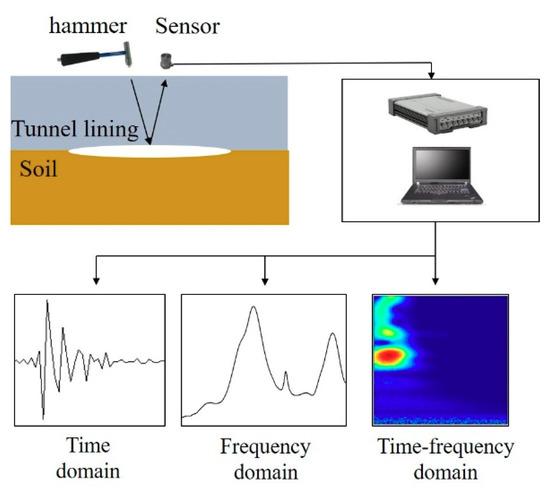
Figure 1.
Test flow chart.
When the IE method is used to detect the thickness of a slab structure, the excited P wave reflects in the slab structure repetitively, which forms a periodic modal related to the thickness of the slab. In turn, the resonance frequency corresponding to the thickness occurs. Therefore, the thickness of a slab structure can be detected by the thickness frequency according to the IE method. When there is a void in the slab, the excited frequency needs to be higher than the thickness frequency. For example, if the velocity of the P wave is 4000 m/s and the depth of the void is 0.2 m, the resonance frequency is calculated as about 10 kHz, which should be contained in the excited frequency range. Therefore, when a void is inside the slab structure, another resonance frequency corresponding to the void can be seen except for the resonance frequency related to the thickness. Then the void can be detected by the IE method by observing the resonance frequencies.
In the situation of detecting voids behind the tunnel lining, the resonance frequencies of the conditions with and without void will be the same, which are both related to the thickness of the tunnel lining. Thus, the void cannot be detected by the difference in the resonance frequency. However, a void can be recognised by IE method due to different responses caused by different reflective ratios. The reflective ratios are caused by the distinct difference in the wave impedance among tunnel lining, soil and air. The wave impedance Z is expressed as:
where is density and is P wave velocity. For the P waves propagate from structure A to structure B, the reflective ratio is expressed as:
where is the reflected amplitude and is the incident amplitude. When is much larger than ZB, the reflected ratio R is closed to −1, which means the amplitude of the reflected wave remains the same, while the phase of the reflected changes. This situation happens at the interface of tunnel lining and air, where almost all of the energy is reflected. When ZA is approximately equal to , the reflected ratio R is closed to 0, which means most of the energy propagates through the interface. This situation is similar to the condition that the tunnel lining is tightly surrounded by the soil.
This section presents the design of a laboratory principle experiment (Figure 2), whereby different signal analysis approaches were then employed to compare the vibration responses for the conditions A and B.
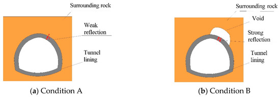
Figure 2.
The basic principle of detecting the void behind tunnel lining by impact-echo (IE) method.
The experiment was carried out in a brick box of size 3.6 × 0.94 × 1.44 m3 (Figure 3a). A rockwool material with a thickness of 0.1 m was placed inside the bunker to weaken the wave reflection at the boundaries. The soil was filled into the bunker. The horseshoe tunnel models were buried in the soil. The cross-sectional size of the tunnel model was 1:16 of a real railway tunnel and the thickness of the tunnel model was 0.025 m (Figure 3b). The tunnel models were made of polyvinyl chloride (PVC) material instead of the concrete. The material coefficients of the soil, the concrete, the PVC, and the air are shown in Table 1. The wave impedance of the PVC and the concrete is within one order of magnitude, which is much larger than the wave impedance of the air. This illustrates that the concrete tunnel can be instead by the PVC, a cheaper material, in this principle experiment. Two different conditions (A and B) were designed. Condition A referred to a tight contact between the tunnel lining and the surrounding soils. The reflected ratio RA at the interface is −0.31. For Condition B, a void behind the tunnel wall was modelled using a pre-embedded empty box of 285 × 145 × 155 mm3 placed between the lining and the soil. The reflected ratio RB at the interface is −1.
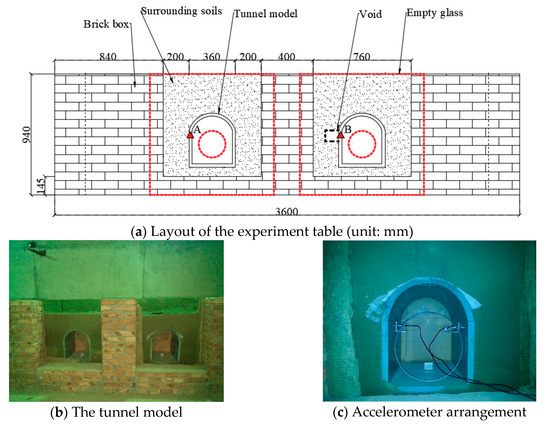
Figure 3.
The test system.

Table 1.
Material parameters used in the principle experiment.
The test system consisted of a hand hammer, two unidirectional accelerometers, a data acquisition instrument with 16 channels, and a computer. The hand hammer, consisted of a hammer head, a force sensor and a hammer body, was used to apply an impact force on the tunnel model. The type of the hammer is Dytran Dytranpulse™5800B4T, developed by the Dytran Instruments company in California, USA. The head of the hammer is made by aluminium with the weight of 100 g and Young’s modulus of 70 GPa. There is a special acceleration compensated piezoelectric force sensor in the hammer head at the striking face, ensuring a smooth frequency spectrum, which is used to measure the value of the impact force. The hammer has a sensitivity of 10 mV/lbf and a maximum force of 1000 lbf. The upper limit of the frequency range is 75 kHz. The type of unidirectional accelerometers is LC0104, developed by LANCE in Ohio, USA. They are used to collect the accelerations perpendicular to the tunnel lining, which has a sample frequency range of 0.5 Hz-9000 Hz, a sensitivity of 100 mV/g, a resolution of 0.0002 g, and an acceleration range of 50g. The type of data acquisition instrument is INV3018C, developed by the China Orient Institute of Noise & Vibration (COINV).
The testing point B was arranged at the tunnel lining behind the empty box on the right tunnel model, while testing point A was arranged at the same location on the left tunnel model, as shown in Figure 3a. According to the thickness and the P wave velocity of the tunnel lining in the test, the thickness resonance frequency is obtained approximately at 28,800 Hz. Since the thickness frequency of the two conditions is the same, this experiment of detecting the void behind tunnel lining does not intend to focus on the amplitude of resonance frequency, but to analyse the dynamic responses of these two conditions in a lower frequency range. The sampling frequency of the accelerometers is set at 2560 Hz. The impact points are 2 cm nearer to the testing points. For each condition, the impact was repeated 10 times. For each time, the peak of impact force is controlled to be close to 400 N, and the sampling frequency is 2560 Hz, as shown in Figure 4. It should be noted that the hammer should be controlled to be perpendicular to the surface of the tested object. To obtain this goal, the coherence function of the response and the force was calculated in each test. If the coherence function was close to 1, the impulse force would be qualified. Otherwise, the data would be removed.
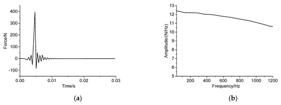
Figure 4.
(a) Time history and (b) spectrum of the impact force.
2.2. Time Domain Analysis
Although the impact forces generated by the hand hammer are controlled within a range, the signals still need to be normalized in order to compare the responses of different conditions. Each impact force and its related response need to multiply by a coefficient , which is obtained as:
where is the peak value of the i-th test. Figure 5 shows the time-domain waveforms of the two conditions, with an intercepted time duration of 0–50 ms. For Condition A, the waveform attenuates smoothly with the amplitude almost decaying to zero in 10 ms. For condition B, an obvious secondary peak occurs at 7 ms, while the minor peaks continuing until 15 ms. This phenomenon of a time-domain waveform with a stronger reflection energy and a prolonged response is suggestive of the existence of a void. It indicates that the stress waves reflect at the interface between the tunnel and the void, and the reflective ratio of concrete–air interface is higher than that of concrete–soil interface.
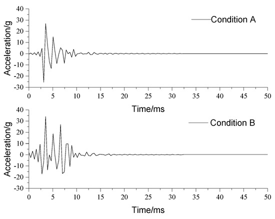
Figure 5.
Time histories of the two conditions (A and B).
The vibration response can be analysed quantitatively using the fractal box-counting dimension method. The concept of fractal dimension was proposed by Mandelbrot [15]. The vibration signal is irregular but self-similar. It occupies a larger area than the one-dimensional line, smaller area than the two-dimensional plane. Its fractal dimension is measured by creating multiscale covers around the signal graph. Square boxes with side length (δ) are used to cover the signal waves on the time-amplitude plane. Then, the number of covered boxes (N) can be obtained (Figure 6). The fractal dimension is defined as:
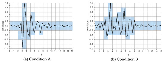
Figure 6.
Number of boxes with side length δ.
For the measured response signals in this paper, square boxes of a series of side lengths (δ1, δ2, ⋯, δn) were used to cover the signal waves on the time-amplitude plane, and then a series of covered box quantities (N1, N2, ⋯, Nn) would be obtained. The minimum δ should be larger than the sampling interval ∆t, because the signal wave was a straight line on every sampling interval. After calculating the fitting line of (−lgδ − lgN), the fractal dimension would be obtained as the slope of the fitting line (Figure 7).
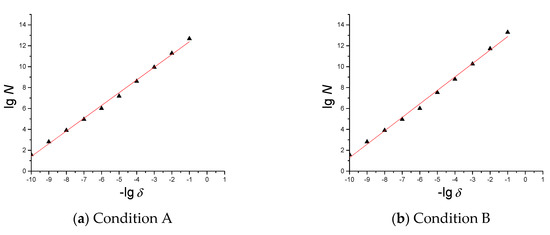
Figure 7.
The fitting lines of (−lgδ − lgN).
The results show that the fractal dimensions of the conditions A and B are 1.221 and 1.288, respectively. This illustrates that when the waveforms of the two conditions are in the coordinate system, with the same time scale and the same amplitude scale, the waveform B is more complicated. Therefore, when the void exists, the fractal dimension is larger, and the waveform in the time domain is more complicated.
2.3. Frequency Domain Analysis
Figure 8 shows the frequency spectra of ten test runs conducted on each of the two conditions. In condition A, all the spectra are similar, and a dominant frequency of approximately 690 Hz is observed. The amplitudes increase steadily between 0 and 500 Hz. In condition B, larger differences among the tested spectra are observed. The dominant frequency remains the same (~690 Hz) as that of condition A. Besides, the amplitude fluctuates between 0 and 500 Hz with two additional peaks between 300 and 500 Hz. For each condition, the average frequency spectra of these test runs are calculated, except for the incoherence test runs (test 1 of condition A and test 4 for condition B), as shown in Figure 8c. The amplitude of condition B is higher than that of condition A in the frequency range of 800 Hz–1100 Hz. There are more dominant frequencies in condition B.
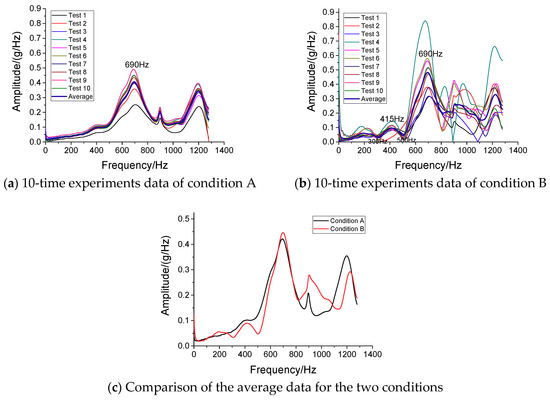
Figure 8.
Fourier spectra for two conditions.
The dynamic stiffness was also used to study the influential differences between the two conditions. It expresses the resistance to deformation under the impact force [16]. In this test, dynamic stiffness reflects the supporting performance of the tunnel-soil structure. The impact force F(t) and the obtained acceleration response a(t) can be transformed into the frequency domain, using Fourier transform, as F(f) and a(f), respectively. The acceleration response is expressed as the superposition of a series of simple harmonic vibrations, so the amplitude of velocity can be represented as:
The velocity admittance is defined as:
Then, the dynamic stiffness can be calculated by:
Figure 9 compares the Kd of the two conditions. The Kd in condition B is lower than condition A. The reason is that the wave propagation in condition B is approximated as guided by a free-free boundary condition while the wave in condition A is guided by a free-constrained boundary condition. This phenomenon shows that the void existence can significantly reduce the dynamic stiffness in most frequencies, which means it reduces the ability of the tunnel structure to resist the load.
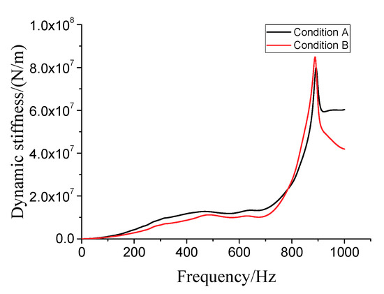
Figure 9.
Dynamic stiffness analysis.
2.4. Time–Frequency Analysis
The frequency-domain analysis is widely used to research the frequency distribution of the signals. However, it is only suitable to the stationary process, not for the non-stationary process. In other words, the frequency domain analysis illustrates the frequency components of the signals but fails to figure out the moment that a certain frequency component appears.
The time–frequency analysis expresses the signal as a function of both time and frequency using the local transform. It helps understand changes in energy with both frequency and time upon the occurrence of a certain frequency. The methods usually adopted for time–frequency analysis are short-time Fourier transform, wavelet transform, Hilbert Huang transform, and so on.
2.4.1. Short-Time Fourier Transform (STFT)
The STFT is used to describe the frequency spectra of local signal sections changing over time. The original signal is first divided into several sections with equal time length by an appropriate sliding time window function . These sections are approximated as stationary processes. Then, by applying the Fourier transform from t to f to each section, the frequency spectra vary with time are obtained. The STFT can be expressed as [17]:
where is the original signal, is the window function centered around zero.
The width of the time window should be properly selected. For example, if a wide time window is selected, the frequency resolution will increase, but the time resolution will decrease, which means these frequency components can only be determined to appear in this wide time band, not a certain instantaneous moment.
Figure 10 shows 3-dimensional (3D) graphs of the two conditions calculated by the STFT. For condition A, three energy peaks can be observed at approximately 700, 900, and 1200 Hz. For condition B, the number of energy peaks increases, and these peaks are all higher than those of condition A. Among them, the energy peak at approximately 700 Hz is the highest. On the low-frequency band between 0 and 100 Hz, the energy distributes widely along the time axis.
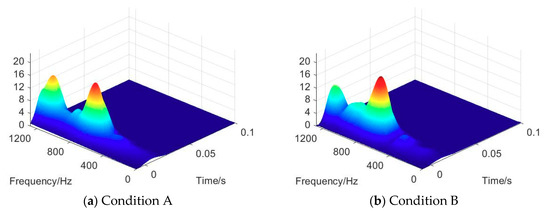
Figure 10.
Time–frequency spectra by STFT.
In summary, when the void exits, the vibration energy becomes stronger, which is indicative of increased reflections of the stress waves from the tunnel-air interface. In addition, more energy moves to the frequency of approximately 700 Hz, which in turn becomes the dominant frequency. It can also be seen that the low-frequency energy attenuates slowly when the void exists.
2.4.2. Wavelet Transform
Wavelet transform uses the mother wavelet function to express the original signal, which can be expressed as:
where is the original signal. The is the mother wavelet function. The a and b are the scaling and translating parameters, respectively. The scaling parameter represents the dilation or compression of the mother wavelet, and the translating parameter determines the mother wavelet moving along the time domain. The dilative mother wavelet corresponds to low-frequency resolution. The compressive mother wavelet corresponds to high-frequency resolution [18]. By calculating the cross-correlation of the original signal and the mother wavelet function under different scales, the frequency components are obtained. The moment that a certain frequency appears is obtained by moving the mother wavelet along the time domain.
For the STFT, when the width of the time window is determined, the resolution of time and frequency on the whole time–frequency range is constant. However, in signal analysing, the high-frequency resolution is needed on the low-frequency range, while the high-time resolution is needed on the high-frequency range. On this aspect, the wavelet transform meets the requirements more closely.
Figure 11 shows the contour maps of the two conditions analysed by Cmor wavelet transform. Except for the characters that are shown in Section 2.4.1 by STFT, new phenomena are found in Figure 11. When the void exists, the frequency components between 1000 Hz and 1200 Hz appears from 0 s to 0.005 s, which is the period of the primary peak in Figure 5. In addition, the frequency components above 1200 Hz occurs from 0.005 s to 0.01 s, which is the period of the secondary peak in Figure 5.
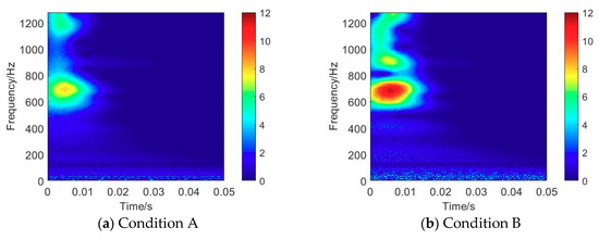
Figure 11.
Time–frequency spectra by wavelet transform.
For the STFT, it could only be roughly determined when the frequency components appear because of the low time resolution. However, for the wavelet transform, the moment that a certain frequency component appears could be clearly figured out. This means that the wavelet transform can tell more detail about the characters.
2.4.3. Hilbert Huang Transform (HHT)
The signal can also be presented in the time–frequency domain using the Hilbert Huang Transform (HHT). The HHT decomposes a signal into intrinsic mode functions (IMFs) along with a trend, and then obtains instantaneous frequency data. Compared to other transforms, HHT is more like an algorithm (an empirical approach) that can be applied to a data set, rather than a theoretical tool. The calculation of the HHT includes two steps: empirical mode decomposition (EMD) and Hilbert transform. By means of EMD, the acceleration data can be decomposed into different simple non-sinusoidal signals, called IMFs [19]. Each IMF is transformed into a time–frequency domain by Hilbert transform, and then the time–frequency spectrum can be obtained after the superposition.
Figure 12 shows the time–frequency spectra of the signals analysed by HHT. The original signals were separated into several IMFs, and the first step of IMF was in the range of 600–1200 Hz. According to the previous analysis, the study would focus on the first-step IMF (600–1200 Hz). For condition A, the vibration energy peak is at 700 Hz and 5 ms, and the energy attenuates significantly after 5 ms, almost approaching zero at 10 ms. For condition B, there are two energy peaks, of which one appears at 1100 Hz and 3.5 ms, while the other one is at 700 Hz and 6 ms. The energy remains high until 10 ms.
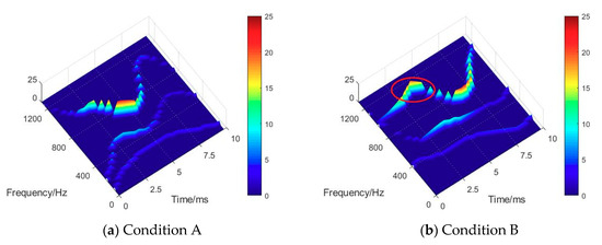
Figure 12.
The time–frequency spectrum.
In summary, when the void exists, another vibration energy peak of 1100 Hz appears at 3.5 ms that is indicative of the reflection of the stress waves at the tunnel-air interface. This phenomenon also explains that the stress waves take longer time to propagate to the soil, which causes the energy peak of 700 Hz to appear 1 ms later in condition B. In addition, the vibration lasts longer when a void exists.
By means of HHT, a signal was separated into several sub-signals dominant in different frequency ranges. As the key frequency band for the sub-signals could be studied individually, the stress wave propagation and the frequency component distribution could be seen clearly, however, it is less holistic because of the separation of the original signal.
The STFT and wavelet transform analysis to focus on the overall vibration energy in a time–frequency plane that could be observed clearly. Similarly, the energy flow between different conditions could also be studied clearly. In principle, unlike the STFT, the wavelet transform can change the scale while analysing different frequencies of the signal. As a result, both high-time and high-frequency resolution can be achieved using wavelet a transform. Based on these aspects, the wavelet analysis method would be chosen for the following numerical study to analyse the signals in time–frequency domains.
3. Numerical Study
The laboratory experiment compared the vibration responses of the two conditions (with and without voids) using IE method. The approach proved to be more satisfactory in the experimental study was employed in the signal analysis using the numerical model, whereby the size and the position of the void were considered.
3.1. Numerical Model
A finite element (FE) model considering the soil, tunnel, and void on the soil-structure interface was built in Midas GTS, shown as Figure 13. The material parameters are shown in Table 2. The coordinate system based on the right-hand rule was shown, and the dimensions of the model were 84 × 84 × 40 m3. The external diameter of the tunnel was 6 m, and the thickness of the tunnel lining was 0.3 m. In order to simulate the wave shape, the size of the mesh needs to be divided smaller than 1/8 of the smallest wavelength, which is expressed as:
where Vs is the shear wave velocity and is the highest analysis frequency, which is 150 Hz in this model. According to the equation, the element of soil should be smaller than 0.25 m and the element of tunnel lining should be smaller than 1.88 m. In this model, the tunnel elements were set at 0.3 m. The soil elements near to the top of the tunnel were set as 0.2 m, and the size was getting bigger as the elements spread from the centre to the boundary of the model. The viscoelastic artificial boundaries were applied to the model to simulate the infinite soil. The viscoelastic artificial boundary is a continuous distributed parallel spring-damping system with calculated stiffness and damping factors. Once these coefficients are input into the Midas GTS software, the equivalent spring-damping elements will be applied on the boundary nodes.
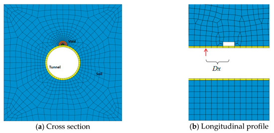
Figure 13.
Tunnel-soil FE model.
Table 2.
Material parameters used in the numerical models.
In the experimental study, the effect of void size on the response was not considered. In contrast, for the numerical study, four conditions with varying void sizes were designed as listed in Table 3. The cross-sections of the voids were fan-shaped with different radius, and their longitudinal length was kept the same as 4 m. An impact force signal was applied on the inner surface of the tunnel lining in the model. The duration of the force was 0.0032 s, and the peak value was 88.26 kN. The frequency range influencing the impact force was between 1 and 150 Hz (Figure 14). The vibration detecting point was 0.1 m close to the impact point. To analyse the effect of the impact-void position, the impact and response points were varied with reference to the centre of void along the outer surface of the tunnel lining. The distance between the impact point and the centre of the void, represented by Dx (Figure 13b), was varied from 1 to 6 m.
Table 3.
Conditions with different void sizes.
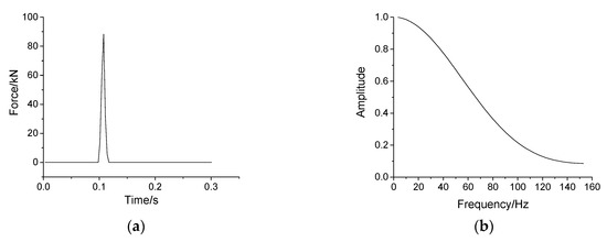
Figure 14.
(a) Time history and (b) spectrum of the impact force.
3.2. Effect of Void Size
Figure 15 illustrates the time histories of the four void size conditions. For condition S0, the acceleration is relatively smaller with a peak value of 6.49 m/s2. For condition S1, the acceleration is larger with a peak value of 7.02 m/s2. This is because, part of the vibration energy is absorbed by the soil beside the void, and part of the energy reflects at the tunnel-void interface. For conditions S2 and S3, with the increase of the void size, the peak value is higher, which means more energy reflects at the interface rather than transmitting into the soil. In short, as the void is larger, the peak value of the waveform is higher, which means more energy is reflected back.
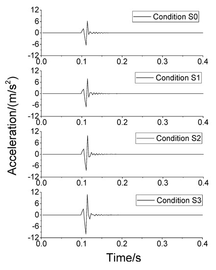
Figure 15.
Time histories of void conditions.
Figure 16 shows normalised Fourier spectra of the four void size conditions. For condition S0, the vibration amplitude distributes in a wide frequency range, and the dominant frequency is not obvious. The normalised peak amplitude is approximately 0.50. With the increase of void size, the amplitude increases, and the dominant frequency can be clearly observed. In general, as the void is bigger, the frequency distributes a narrower range, and the dominant frequency at 90 Hz is more obvious.
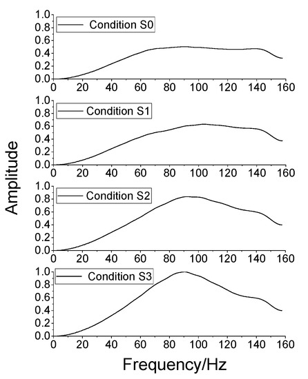
Figure 16.
Normalised Fourier spectra of void conditions.
Figure 17 illustrates that the dynamic stiffness varies with frequency for the four conditions. With the increase of void size, the dynamic stiffness decreases in almost all the frequencies.
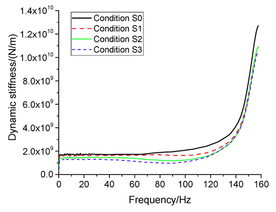
Figure 17.
Dynamic stiffness analysis.
Figure 18 shows the colour contours of the wavelet spectra for the four void size conditions. With the increase of the void size, the spectrum becomes larger, and an increasing energy concentration can be obviously found. More energy tends to concentrate over 80–120 Hz, which in turn becomes the dominant frequency band. The vibration duration is longer especially in the range of 60–120 Hz. While the frequency is lower, the vibration energy lasts longer.
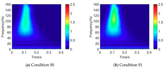
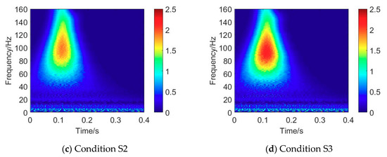
Figure 18.
Wavelet spectra for different void size conditions.
When the impulse force is applied to the tunnel, the P wave propagates into the structure as a semi-spherical wave. Figure 19 shows a sectional draw of the reflection of the stress wave with different void sizes. According to the wave impendence introduced in Section 2.1, there is a strong reflection (red part) in the tunnel-void interface and a weak reflection (blue part) in the tunnel-soil interface. While the void becomes larger, the angle of the red part is larger, which means more energy reflects back and the attenuation lasts longer. This may cause the spectrum becomes larger in proportion to the void size.
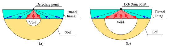
Figure 19.
The reflections of P wave in the conditions with (a) small void and (b) big void.
3.3. Effect of Distance between Impact and Void Position
When the impact location is far from the void, the void existence is not distinctly recognised. Accordingly, in this subsection, different impact positions were analysed. The distance between the impact location and the void centre was defined as Dx, which was varied from 0 to 6 m for the different void size conditions. Figure 20 shows the dynamic stiffness Kd of the responses. The average values of the dynamic stiffness were calculated in the range of 20–100 Hz due to the steady amplitudes.
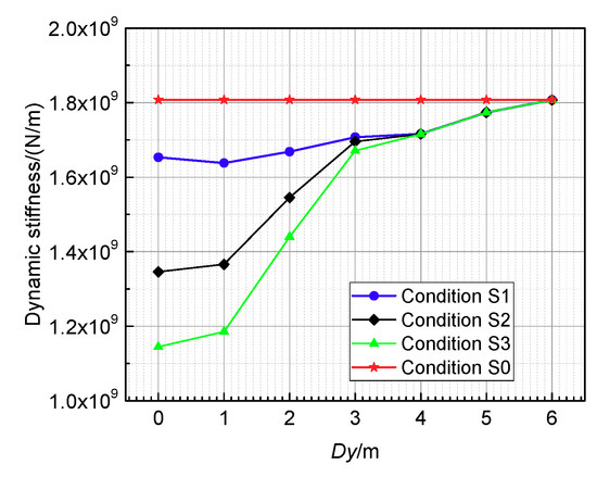
Figure 20.
Dynamic stiffness of different void positions.
For condition S0, Kd is not affected by Dx. When Dx changes from 0 to 1 m, in the range of void size, Kd for condition S1 decreases slightly, while for conditions S2 and S3 increase slightly.
For conditions S1, S2, and S3, when Dx changes from 1 to 3 m, Kd increases significantly. That is, the dynamic stiffness changes quickly when the impact point moves through the void edge. When Dx changes from 3 to 6 m, Kd increases slowly. The dynamic stiffness for void conditions becomes almost the same as that of the non-void condition when Dx reaches to 6 m.
4. Conclusions
To investigate the effect of a void behind a tunnel lining using the IE method, both experimental and numerical studies were performed. The different signal analysis approaches were compared, and the influence of the void size and impact-void position were analysed. The following conclusions can be drawn:
- In the analysis of the vibration response in the time, frequency, and time–frequency domains, the fractal box-counting dimensions and dynamic stiffness can be used for void recognition quantitatively, and the wavelet analysis can provide a relatively better visual energy distribution among the different time–frequency analysis approaches.
- When the void is larger, the dynamic stiffness decreases. When the impact location is beyond the range of void size, the dynamic stiffness changes quickly.
By comparison of different signal analysis approaches, wavelet transform is believed to be the most appropriate one to show the energy flow during the void state changing. Besides, the dynamic stiffness could be used to detect the void position accurately.
Author Contributions
Data curation, R.C. and R.L.; formal analysis, R.C. and C.N.; funding acquisition, M.M.; investigation, R.L. and C.N.; methodology, M.M.; project administration, M.M.; software, R.C.; supervision, M.M.; writing—original draft, R.C.; writing—review & editing, R.C. and M.M.
Funding
This research was funded by fundamental research funds for the central universities, grant number 2018JBM036 and the research funding of China academy of railway sciences, grant number 2018YJ164.
Conflicts of Interest
The authors declare no conflict of interest. The funders played role in the design of the study, the collection and the decision to publish the results.
References
- Lalagüe, A.; Lebens, M.A.; Hoff, I.; Grøv, E. Detection of Rockfall on a Tunnel Concrete Lining with Ground-Penetrating Radar (GPR). Rock Mech. Rock Eng. 2016, 49, 2811–2823. [Google Scholar] [CrossRef]
- Cardarelli, E.; Marrone, C.; Orlando, L. Evaluation of tunnel stability using integrated geophysical methods. J. Appl. Geophys. 2003, 52, 93–102. [Google Scholar] [CrossRef]
- Huang, J.; Qi, H.; Diao, Z. Application of ultrasonic-rebound combined method in concrete strength test for tunnel secondary lining. Water Resour. Hydropower Northeast 2011, 23. [Google Scholar] [CrossRef]
- Wang, W.; Xiang, Y. Non-destructive testing and its application in tunnels. J. Railw. Eng. Soc. 2001, 3, 85–88. [Google Scholar]
- Sansalone, M.; Carino, N. Detecting Voids in Metal Tendon Ducts using the Impact-Echo Method. Mater. J. Am. Concr. Inst. 1992, 89, 8. [Google Scholar]
- Sansalone, M.J.; Streett, W.B. Impact-Echo: Nondestructive Evaluation of Concrete and Masonry; Bullbrier Press: Jersey Shore, PA, USA, 1997; ISBN 0961261064. [Google Scholar]
- Ni, S.-H.; Lehmann, L.; Charng, J.-J.; Lo, K.-F. Low-strain integrity testing of drilled piles with high slenderness ratio. Comput. Geotech. 2006, 33, 283–293. [Google Scholar] [CrossRef]
- Cheng, C.-C.; Yu, C.-P.; Liou, T. Evaluation of interfacial bond condition between concrete plate-like structure and substrate using the simulated transfer function derived by IE. NDT E Int. 2009, 42, 678–689. [Google Scholar] [CrossRef]
- Aggelis, D.; Shiotani, T.; Kasai, K. Evaluation of grouting in tunnel lining using impact-echo. Tunn. Undergr. Space Technol. 2008, 23, 629–637. [Google Scholar] [CrossRef]
- Song, K.-I.; Cho, G.-C. Bonding state evaluation of tunnel shotcrete applied onto hard rocks using the impact-echo method. NDT E Int. 2009, 42, 487–500. [Google Scholar] [CrossRef]
- Song, K.-I.; Cho, G.-C. Numerical study on the evaluation of tunnel shotcrete using the Impact-Echo method coupled with Fourier transform and short-time Fourier transform. Int. J. Rock Mech. Min. Sci. 2010, 47, 1274–1288. [Google Scholar] [CrossRef]
- Davis, A.G.; Lim, M.K.; Petersen, C.G. Rapid and economical evaluation of concrete tunnel linings with impulse response and impulse radar non-destructive methods. NDT E Int. 2005, 38, 181–186. [Google Scholar] [CrossRef]
- Ryden, N.; Aurell, O.; Nilsson, P.; Hartlén, J. Impact echo Q-factor measurements towards non-destructive quality control of the backfill in segmental lined tunnels. In Nondestructive Testing of Materials and Structures; Springer: Berlin/Heidelberg, Germany, 2013; pp. 915–919. [Google Scholar] [CrossRef]
- Sansalone, M.; Carino, N. Impact-Echo: A Method for Flaw Detection in Concrete Using Transient Stress Waves; National Bureau of Standards: Gaithersburg, MD, USA, 1986. [Google Scholar] [CrossRef]
- Mandelbrot, B.B. The Fractal Geometry of Nature; WH Freeman: New York, NY, USA, 1983; Volume 173, ISBN 0716711869. [Google Scholar]
- Ma, M.; Liu, J.; Ke, Z.; Gao, Y. Bearing Capacity Estimation of Bridge Piles Using the Impulse Transient Response Method. Shock Vib. 2016, 2016, 1–8. [Google Scholar] [CrossRef]
- Ge, Z.; Chen, Z. Matlab Guide to Time-Frequency Analysis; Posts & Telecom Press: Beijing, China, 2006; ISBN 9787115141132. [Google Scholar]
- Lee, I.-M.; Han, S.-I.; Kim, H.-J.; Yu, J.-D.; Min, B.-K.; Lee, J.-S. Evaluation of rock bolt integrity using Fourier and wavelet transforms. Tunn. Undergr. Space Technol. 2012, 28, 304–314. [Google Scholar] [CrossRef]
- Shi, Z.; Liu, L.; Peng, M.; Liu, C.; Tao, F.; Liu, C. Non-destructive testing of full-length bonded rock bolts based on HHT signal analysis. J. Appl. Geophys. 2018, 151, 47–65. [Google Scholar] [CrossRef]


© 2019 by the authors. Licensee MDPI, Basel, Switzerland. This article is an open access article distributed under the terms and conditions of the Creative Commons Attribution (CC BY) license (http://creativecommons.org/licenses/by/4.0/).