High Precision Adaptive Robust Neural Network Control of a Servo Pneumatic System

Abstract

In this paper, an adaptive robust neural network controller (ARNNC) is synthesized for a single-rod pneumatic actuator to achieve high tracking accuracy without knowing the bounds of the parameters and disturbances. The ARNNC control framework integrates adaptive control, robust control, and neural network control intelligently. Adaptive control improves the precision of dynamic compensation with parametric estimation, and robust control attenuates the effect of unmodeled dynamics and unknown disturbances. In reality, the unmodeled dynamics of the complicated pneumatic systems and unpredictable disturbances in working conditions affect the tracking precision. However, these cannot be expressed as an exact formula. Therefore, the real-time learning radial basis function (RBF) neural network component is considered for better compensation of unmodeled dynamics, random disturbances, and estimation errors of the adaptive control. Although the bounds of the parameters and disturbances for the pneumatic systems are unknown, the prescribed transient performance and final tracking accuracy of the proposed method can be still achieved with fictitious bounds. Asymptotic tracking performance can be acquired under the provided circumstance. The comparative experiments with a pneumatic cylinder driven by proportional direction valve illustrate the effectiveness of the proposed ARNNC as shown by a high tracking accuracy is achieved.

1. Introduction

Pneumatic actuators have been widely used in industrial applications due to the advantages of having a high power/mass ratio, being low cost, clean, and easily serviced [1,2,3]. Some examples are pneumatic force actuator systems [1,4], positioning control systems [5], and rehabilitation devices [6]. However, the dynamics of the pneumatic system are complicated, including the nonlinearities of pressure dynamics, the compressibility of air, unmodeled friction, and random disturbances, etc. The unmodeled dynamics, disturbances, and inaccurate mathematic models result in achieving precise motion control of pneumatic cylinders being a challenging task.

The linear control strategy and modified linear control techniques [5,7,8] are widely applied to the pneumatic systems, but the strong nonlinear dynamics of pneumatic systems restrict the capability of a linear controller in achieving a high precision tracking performance. Therefore, the model-based control strategy is considered for pneumatic systems [9]. The sliding mode control [10,11,12] method is introduced to pneumatic systems for strong robustness; however, it has limited capacity to compensate for nonlinear dynamics. In addition, the backstepping [13] technique is used for controller design and stability analysis of the pneumatic systems. The adaptive control strategy [14] is used for pneumatic systems to obtain a more precise model compensation but is vulnerable to disturbances. Adaptive robust control (ARC) [15,16] takes advantages of robust control and adaptive control to acquire robustness and better tracking performance. Zhu et al. [17,18] devised the adaptive robust controller for a parallel manipulator driven by pneumatic muscles, and significant performance was achieved. The ARC scheme also serves to design a controller for position tracking of the pneumatic cylinder [19]. Although the performance of ARC controller for pneumatic systems is improved compared with other nonlinear controllers, several problems exist. First, the ARC improves the model compensation by the accurate estimation of unknown parameters which needs a known structure for the system dynamics. However, the unmodeled dynamics of complex pneumatic motion progress is hard to describe as a known structure due to the lack of knowledge concerning physical phenomena, including friction force, heat transfer, random disturbances, etc. Moreover, too complicated mathematical models are not convenient for controller design. Second, the existing ARC controllers for pneumatic systems are requested for known bounds for all unknown parameters and these are not easy to acquire. Furthermore, too large a range for bounds of unknown parameters will lead to a saturation problem [20].

Fortunately, neural networks (NN) have been used in controller design for their excellent ability to approximate arbitrary unknown nonlinearities [21], including the unmodeled dynamics and random disturbances. Therefore, NN controllers have been designed for high nonlinear pneumatic systems to obtain better model compensation [22,23,24,25].

However, these NN controllers either need off-line training or have too many parameters to regulate since they do not fully utilize the knowledge about pneumatic systems. Therefore, a combination of ARC control philosophy and NN is a practical way to improve the performance of pneumatic systems. A control scheme with NN based ARC [26,27] was proposed for dealing with the unknown nonlinearities of the system and was applied to a linear motor. The mentioned NN based ARC suffered the difficulties of activation function selection, and the performance was not much better than ARC. A neural network learning ARC [28] controller with disturbances rejection was also synthesized for the industrial linear motor. Comparative experimental results showed better compensation of this data-driven RBF neural network when dealing with unmodeled dynamics and random disturbances.

In this paper, an extended study of the adaptive robust neural network controller (ARNNC) for high precision tracking control of a pneumatic cylinder system is proposed. The main points of the control strategy are as follows:

(a)

The ARNNC approach is used to estimate not only the unknown parameters of the known structure part but to approximate the unmodeled dynamics, random disturbances, and residual estimation errors. With these compensations, a better trajectory tracking performance of the pneumatic system is achieved.

(b)

Unlike the multilayer NN [26,27], the chosen RBF NN is designed based on the reference trajectory and is easy to handle [28].

(c)

A discontinuous projection with fictitious bounds of unknown parameters and NN weights guarantee the range of parameters and weights. Backstepping techniques are also used for the controller design of pneumatic systems. Prescribed transient tracking performance and final tracking accuracy can be still obtained with the fictitious bounds. In addition, if the parameters and weights lie in assumed bounds, an asymptotic stable state can be acquired in the presence of parametric uncertainties only.

A pneumatic cylinder is chosen as the plant for comparative studies with trajectory tracking control. To test the designed ARNNC controller, experiments with different trajectories, loads, and disturbances were carried out. The results verify the efficiency of the proposed controller.

The paper is organized as follows. In Section 2, an appropriate mathematic model for the pneumatic cylinder system is set up, and problem formulation is carefully done. The ARNNC approach for the pneumatic system is described in Section 3. Experimental results are shown in Section 4. Finally, Section 5 concludes the paper.

2. Dynamics and Problem Formulation

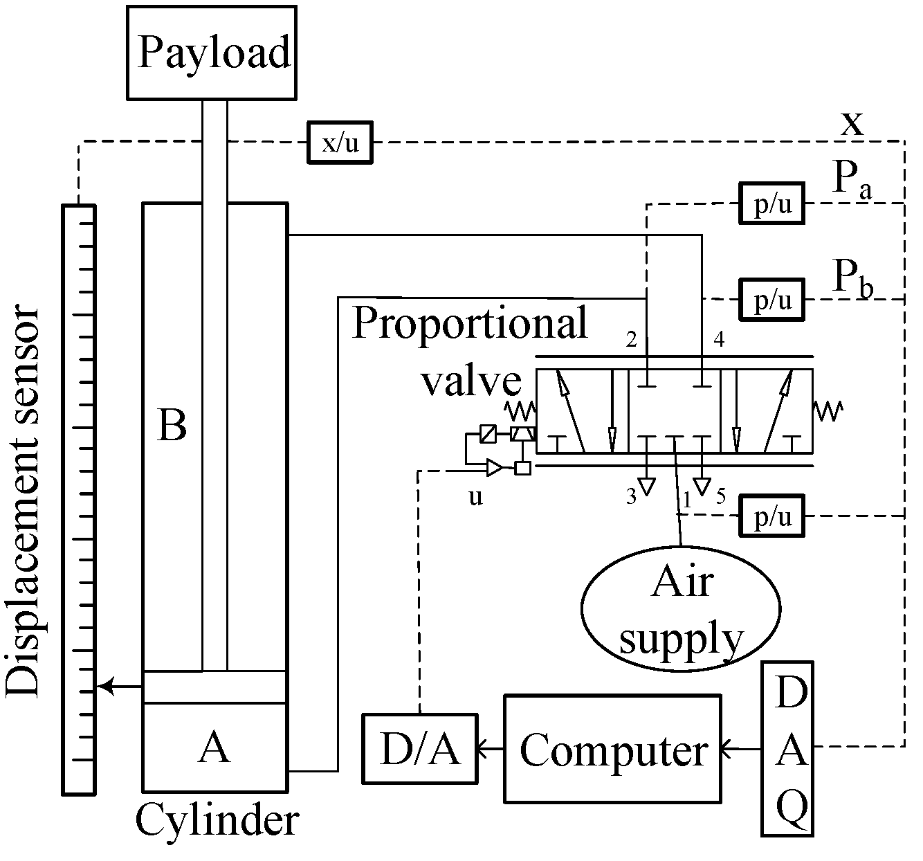
A single-rod pneumatic cylinder depicted in Figure 1 is considered as the object in this paper. According to [19], the dynamics of piston movement of the system can be described as:

$$M\ddot{x}=(p_a-p_0)S_a-(p_b-p_0)S_b-F_g-F_f+f_0+{\tilde{f}}_0,$$

(1)

where $M$ represents the inertia of piston and lumped payload; $x$ is the displacement of the piston, $p_0$, $p_a$, and $p_b$ represent the absolute pressure of the atmosphere, cylinder chamber $A$ and $B$, respectively. $S_a$ and $S_b$ are the effective areas of the forward and backward chamber; $F_g$ is the component of gravitational force along the direction of the piston motion; $F_f$ is the friction force which is a combination of viscous friction $b\dot{x}$ in which $b$ represents the viscous friction coefficient and the Coulomb friction $F_c$, i.e., $F_c=A_f{S}_f(\dot{x})$; and $(f_0+{\tilde{f}}_0)$ represents the lumped modeling errors including uncertain nonlinearities, such as unmodeled friction forces, and external disturbances in which $f_0$ represents the nominal value.

The complete pneumatic cylinder dynamics are described in [29], which is too complex for controller design. For simplicity, suppose the gas temperature follows the polytropic law [30] and can be written as:

$$\{\begin{array}{l}{T}_l=T_r{(\frac{p_l}{p_{eb}})}^{\frac{n-1}{n}},p_{eb}=0.8077p_r\\ \frac{d{p}_l}{dt}=\frac{\gamma R}{V_l}({\dot{m}}_{lin}{T}_r-{\dot{m}}_{lout}{T}_l)-\frac{\gamma p_l}{V_l}\frac{d{V}_l}{dt}+\frac{\gamma -1}{V_l}{\dot{Q}}_l+f_{lm}+{\tilde{f}}_{lm}\end{array},$$

(2)

where $l=a,b$ which represent each chamber of cylinder; $T_l$ is the temperature of gas inside the chamber; $T_r$ is the temperature of air supply; $p_{eb}$ is the equilibrium pressure when the spool of the control valve is at the central position; $n=1.35$ is the polytropic coefficient; $p_r$ is the pressure of the air supply; $\gamma$ is the specific heat ratio; $R$ is the gas constant; ${\dot{m}}_{lin}$, ${\dot{m}}_{lout}$ represent supply flow and return flow, respectively; $V_l=V_{0l}+S_l(0.5L\pm x)$ is the volume of the chamber which $V_{0l}$ is the dead volume and $L$ is the stroke; ${\dot{Q}}_l$ is the heat transfer of air and the inside barrel of cylinder; $(f_{lm}+{\tilde{f}}_{lm})$ represents the lumped modeling error including neglected temperature dynamics, uncertainties, and random disturbances in which $f_{lm}$ is the nominal value.

The dynamic features of MPYE valve spool will not be taken into consideration since it has a much high bandwidth than the frequency of the pneumatic system; the relationship between mass flow and the control input voltage can be established as [19]:

$$\begin{array}{l}q=S(u)K_q(p_u,p_d,T_u)=\\ \{\begin{array}{ll}S(u)C_d{C}_1\frac{p_u}{\sqrt{T_u}};& \frac{p_d}{p_u}\le p_{cr}\\ S(u)C_d{C}_1\frac{p_u}{\sqrt{T_u}}\sqrt{1-{\left(\frac{(\frac{p_d}{p_u}-p_{cr})}{(1-p_{cr})}\right)}^2}& p_{cr}<\frac{p_d}{p_u}<1\end{array}\end{array},$$

(3)

where $q$ is the mass flow; $u$ is the voltage and $S\left(u\right)$ is the effective area of the orifice; $p_u$ is the pressure of the upstream flow and $p_d$ is the pressure of the downstream flow; and $p_{cr}$ is the critical pressure ratio.

The state space model of the whole pneumatic system is described by [19]

$$\{\begin{array}{l}{\dot{x}}_1=x_2\\ {\dot{x}}_2={\theta }_1\left({\overline{S}}_a(x_3-k_{S_a/S_b}{x}_4)-F\right)+{\theta }_2+{\tilde{f}}_1\\ {\dot{x}}_3=\frac{\gamma R}{L_P{V}_a}{\dot{m}}_a-\frac{\gamma S_a}{V_a}{x}_2{x}_3+\frac{\gamma -1}{L_P{V}_a}{\dot{Q}}_a+{\theta }_3+{\tilde{f}}_a\\ {\dot{x}}_4=\frac{\gamma R}{L_P{V}_b}{\dot{m}}_b+\frac{\gamma S_b}{V_b}{x}_2{x}_4+\frac{\gamma -1}{L_P{V}_b}{\dot{Q}}_b+{\theta }_4+{\tilde{f}}_b\end{array},$$

(4)

where $\left[x_1,x_2,x_3,x_4\right]=\left[x,\dot{x},{\overline{p}}_a,{\overline{p}}_b\right]$; ${\overline{p}}_l=p_l/L_P$ for $l=a,b$, and $L_P={10}^5$ is a constant factor; $k_{S_a/S_b}$ is the ratio of $S_a$ and $S_b$; ${\overline{S}}_a=S_a{L}_p$; $F=b{x}_2+A_f{S}_f(x_2)+p_0(S_a-S_b)$; ${\tilde{f}}_1={\tilde{f}}_0/M$; ${\dot{m}}_l=({\dot{m}}_{lin}{T}_r-{\dot{m}}_{lout}{T}_l)$; ${\tilde{f}}_l={\tilde{f}}_{lm}/L_p$; $\theta ={[{\theta }_1,{\theta }_2,{\theta }_3,{\theta }_4]}^T={[1/M,(f_0+F_g)/M,f_{am}/L_p,f_{bm}/L_p]}^T$.

For simplicity, the following nomenclature $\widehat{\ast }$ and $\tilde{\ast }$ are used to represent the estimation and error of $\ast$ and $\tilde{\ast }=\widehat{\ast }-\ast$, ${\ast }_i$ is the $i_{th}$ component of $\ast$, ${\ast }_{\max }$ and, ${\ast }_{\min }$ represent the maximum and minimum value of $\ast$.

Let $x_{1r}$ be the tracking trajectory. This paper aims to synthesize a control law for a single-rod pneumatic cylinder system to follow $x_{1r}$ as closely as possible and to determine how to compensate unmodeled dynamics, disturbances, and residual estimation errors with a NN under the ARC frame.

Assumption 1. 

Parameters of system are bounded,

$$\left|{\theta }_{\mathrm{i}}\right|<{\delta }_{i}i=1,2,3,4$$

(5)

the bounds of${\theta }_1$are designed as$0<{\theta }_{1\min }<{\widehat{\theta }}_1<{\theta }_{1\max }={\delta }_1$and the bounds for${\theta }_2,{\theta }_3,{\theta }_4$are unknown but exist.

Assumption 2. 

The optimal weights of the neural network are unknown but exist in the unknown bounds,

$$W_i{}^{{}^{★}}\le {\delta }_{i}i=p,q$$

(6)

where$W_i{}^{{}^{★}}$are the optimal weights of the neural network and${\delta }_i$are unknown bounds for the weights.

3. ARNNC of Single-Rod Pneumatic Cylinders

In this section, an ARNNC control strategy for pneumatic systems will be proposed. As shown in Figure 2, the presented design methodology integrates ARC philosophy and the NN philosophy intelligently. The ARC part obtains an accurate parameters’ estimation by adaptation and closed-loop stability of the whole system by robust feedback terms. The NN provides an uncertain compensation for the unmodeled dynamics of complicated pneumatic systems, unpredictable disturbances in working conditions, and estimation errors of the adaptive part. The following section will describe the ARNNC control scheme for a single-rod cylinder pneumatic system in detail.

3.1. ARC Control Part

In this part, the ARC is designed to compensate the parameter uncertainties of the pneumatic cylinder dynamics and acquire a stable feedback control.

Although the bounds $\delta$ of ${\theta }_i,i>1$ are unknown, we define $\widehat{\delta }$ as a fixed estimation of $\delta$ and the discontinuous projection $\dot{\widehat{\theta }}=Proj(\Sigma \sigma )$ is defined as in [20,31] which guarantees the following property:

$$\begin{array}{l}P1\left|{\widehat{\theta }}_i\right|<{\widehat{\delta }}_{i}i=2,3,4\mathrm{and}{\theta }_{1\min }<{\widehat{\theta }}_1<{\theta }_{1\max }={\widehat{\delta }}_1\\ P2{\tilde{\theta }}^T\left(Proj\left(\Sigma \sigma \right)-\sigma \right)\le 0\forall \sigma \end{array},$$

(7)

where $\Sigma$ is a diagonal matrix and $\sigma$ is the adaptation function.

Defining a sliding surface such as:

$$s_2\left(t\right)=\left(\frac{d}{dt}+{\lambda }_1\right)s_1\left(t\right),$$

(8)

where $s_1\left(t\right)=x_1\left(t\right)-x_{1\mathrm{r}}\left(t\right)$ is the position tracking error and ${\lambda }_1$ is any positive constant. And the dynamics of $s_2$ are described as

$${\dot{s}}_2={\theta }_1\left({\overline{S}}_a(x_3-k_{S_a/S_b}{x}_4)-F\right)+{\theta }_2+{\tilde{f}}_1-{\dot{a}}_r$$

(9)

Design $p$ as the virtual input for driven force $(x_3-k_{S_a/S_b}{x}_4)$, and synthesize the virtual control law $p$ and adaptation function ${\sigma }_2$ according to [32,33,34],

$$p=p_a+p_s+p_{nn},$$

(10)

$$p_a=-\frac{1}{{\widehat{\theta }}_1{\overline{S}}_a}\left({\widehat{\theta }}_2-{\dot{a}}_r\right)+\frac{F}{{\overline{S}}_a},$$

(11)

$$p_s=-\frac{1}{{\theta }_{1\min }{\overline{S}}_a}{\lambda }_2{s}_2,$$

(12)

$${\sigma }_2=w_2{\psi }_2{s}_2,$$

(13)

where ${\dot{a}}_r={\ddot{x}}_{1r}-{\lambda }_1{\dot{s}}_1$; $w_2$ is the weighting factor; ${\psi }_2=[\left({\dot{a}}_r-{\widehat{\theta }}_2\right)/{\widehat{\theta }}_1,1,0,{0]}^T$; ${\lambda }_2$ is a positive constant for feedback term $p_s$; $p_{nn}$ is the NN compensator to be demonstrated in the next section. The optimal value $p^{★}$ with the following properties [28] for $p_{nn}$ exists due to the boundedness condition (5) and P1 of (7),

$$\begin{array}{l}1.{\theta }_1{\overline{S}}_a(p^{★}+\frac{1}{{\theta }_{1\min }{\overline{S}}_a}{\lambda }_{2s}{s}_2)-{\psi }_2{}^T\tilde{\theta }+{\tilde{f}}_1<{\epsilon }_{21}\\ 2.s_2({\theta }_1{\overline{S}}_a{p}^{★}-{\psi }_2{}^T\tilde{\theta }+{\tilde{f}}_1)<{\epsilon }_{22}\\ 3.s_2{p}^{★}<0\end{array},$$

(14)

where ${\epsilon }_{21},{\epsilon }_{22}$ are small real positive constants. Noting (14) $p^{★}+\frac{1}{{\theta }_{1\min }{\overline{S}}_a}{\lambda }_{2s}{s}_2$ is considered to compensate for the unmodeled dynamics, random disturbances ${\tilde{f}}_1$, and the estimated errors of the adaptive part ${\psi }_2{}^T\tilde{\theta }$, and $-\frac{1}{{\theta }_{1\min }{\overline{S}}_a}{\lambda }_{2s}{s}_2$ is the robust term explained in the next subsection.

Let $s_3=\left(x_3-k_{S_a/S_b}{x}_4\right)-p$, the dynamics of $s_3$ are given as:

$${\dot{s}}_3=q-(\frac{\gamma S_a}{V_a}{x}_2{x}_3+k_{S_a/S_b}\frac{\gamma S_b}{V_b}{x}_2{x}_4)+\frac{\gamma -1}{L_p{V}_a}{\dot{Q}}_a-k_{S_a/S_b}\frac{\gamma -1}{L_p{V}_b}{\dot{Q}}_b+{\theta }_3-k_{S_a/S_b}{\theta }_4+{\tilde{f}}_a-k_{S_a/S_b}{\tilde{f}}_b-{\dot{p}}_c-{\dot{p}}_u$$

(15)

where $q=\frac{\gamma R}{L_p{V}_a}({\dot{m}}_{ain}{T}_r-{\dot{m}}_{aout}{T}_a)-k_{S_a/S_b}\frac{\gamma R}{L_p{V}_b}({\dot{m}}_{bin}{T}_r-{\dot{m}}_{bout}{T}_b)$; ${\dot{p}}_c=\frac{\partial p}{\partial x_1}{\dot{x}}_1+\frac{\partial p}{\partial x_2}{\widehat{\dot{x}}}_2+\frac{\partial p}{\partial \widehat{\theta }}\widehat{\dot{\theta }}+\frac{\partial p}{\partial {\widehat{W}}_p}{\widehat{\dot{W}}}_p+\frac{\partial p}{\partial g_p}{\dot{g}}_p+\frac{\partial p}{\partial t}$, and ${\dot{p}}_u=\frac{\partial p}{\partial x_2}{\tilde{\dot{x}}}_2$ represents the calculated and uncalculated part of $\dot{p}$, respectively. $\frac{\partial p}{\partial {\widehat{W}}_p}{\widehat{\dot{W}}}_p+\frac{\partial p}{\partial g_p}{\dot{g}}_p$ is the derivative of ${\widehat{W}}_p{g}_p$ which will be explained later.

Design a virtual input for $q$ and adaptation function for ${\sigma }_3$ as:

$$q=q_a+q_s+q_{nn},$$

(16)

$$q_a=-q_r-{\psi }_3{}^T\widehat{\theta },$$

(17)

$$q_s=-{\lambda }_3{s}_3,$$

(18)

$${\sigma }_3=w_3{\psi }_3{s}_3,$$

(19)

where $q_r=-(\frac{\gamma S_a}{V_a}{x}_2{x}_3+k_{S_a/S_b}\frac{\gamma S_b}{V_b}{x}_2{x}_4)+\frac{\gamma -1}{S_p{V}_a}{\dot{Q}}_a-k_{S_a/S_b}\frac{\gamma -1}{S_p{V}_b}{\dot{Q}}_b-{\dot{p}}_c+\frac{\partial p}{\partial x_2}{\widehat{\dot{x}}}_2$; ${\psi }_3=[\frac{w_2}{w_3}{\overline{S}}_a{s}_2{s}_3-\frac{\partial p}{\partial x_2}({\overline{S}}_a(x_3-k_{S_a/S_b}{x}_4)-F),-$$\frac{\partial p}{\partial x_2},1,-k_{S_a/S_b}{]}^T$; $w_3$ is the weight constant; ${\lambda }_3$ is a positive constant for feedback term $q_s$; $q_{nn}$ is the NN compensator to be demonstrated in the next subsection. The optimal value $q^{{}^{{}^{★}}}$ for $q_{nn}$ can be designed similar to (14) with the following properties [28]:

$$\begin{array}{l}1.(q^{★}+{\lambda }_{3s}{s}_3)-{\psi }_3{}^T\tilde{\theta }+{\tilde{f}}_a-k_{S_a/S_b}{\tilde{f}}_b-{\dot{p}}_u<{\epsilon }_{31}\\ 2.s_3(q^{★}-{\psi }_3{}^T\tilde{\theta }+{\tilde{f}}_a-k_{S_a/S_b}{\tilde{f}}_b-{\dot{p}}_u)<{\epsilon }_{32}\\ 3.s_3{q}^{★}<0\end{array},$$

(20)

where ${\epsilon }_{31},{\epsilon }_{32}$ are small real positive constants. Noting (14) $q^{★}+{\lambda }_{3s}{s}_3$ is considered to compensate for the unmodeled dynamics and random disturbances ${\tilde{f}}_a,{\tilde{f}}_b,{\dot{p}}_u$, and the modeling errors of adaptive estimation ${\psi }_3{}^T\tilde{\theta }$, and $-{\lambda }_{3s}{s}_3$ is the robust term explained in the next subsection.

At last, control input can be calculated with Equation (3) and the equation of effective orifice area against $u$ [29].

Theorem 1. 

Under the assumptions A1, A2, and with control law (10), (16), and adaptation law$\sigma ={\sigma }_2+{\sigma }_3$for${\theta }_1,{\theta }_2,{\theta }_3,{\theta }_4$, the following properties can be obtained:

A. All signals of the whole closed system are bounded. Furthermore, the positive definite function is defined by

$$V_s=\frac{1}{2}{w}_2{s}_2{}^2+\frac{1}{2}{w}_3{s}_3{}^2$$

(21)

is bounded by

$$V_s\le e^{-\lambda t}{V}_s(0)+\frac{\epsilon }{\lambda }(1-e^{-\lambda t}),$$

(22)

where$\lambda =\min \{2{\theta }_1{\lambda }_2,2{\lambda }_3\}$; $\epsilon =w_2{\epsilon }_{22}+w_3{\epsilon }_{32}$.

B. In addition, provided$\forall i=1,a,b$that$f_i=0$and the$\theta$exist in the fictitious bound$\widehat{\delta }$, the asymptotic stable state can be achieved.

Proof of Theorem 1. 

The derivative of $V_s$ is given by

$$\begin{array}{l}{\dot{V}}_s=w_2{s}_2{\dot{s}}_2+w_3{s}_3{\dot{s}}_3\\ =w_2{s}_2({\theta }_1({\overline{S}}_a(p+s_3)-F)+{\theta }_2+{\tilde{f}}_1-{\dot{a}}_r)+w_3{s}_3(q+q_r+{\psi }_3{}^T\theta -\frac{w_2}{w_3}{\overline{S}}_a{s}_2{s}_3{\theta }_1+{\tilde{f}}_a-k_{S_a/S_b}{\tilde{f}}_b-{\dot{p}}_u)\end{array}$$

(23)

Taking $p$ and $q$ into (22) and considering 2 of (14) and (20),

$$\begin{array}{l}{\dot{V}}_s=-{\theta }_1{\lambda }_2{w}_2{s}_2{}^2+w_2{s}_2({\theta }_1{p}^{★}{\overline{S}}_a-{\psi }_2{}^T\tilde{\theta }+{\tilde{f}}_1)-{\lambda }_3{w}_3{s}_3{}^2+w_3{s}_3(q^{★}-{\psi }_3{}^T\tilde{\theta }+{\tilde{f}}_a-k_{S_a/S_b}{\tilde{f}}_b-{\dot{p}}_u)\\ \le -{\theta }_1{\lambda }_2{w}_2{s}_2{}^2-{\lambda }_3{w}_3{s}_3{}^2+w_2{\epsilon }_{22}+w_3{\epsilon }_{32}\le -\lambda V_s+\epsilon \end{array}$$

(24)

which leads to (22) and part A of Theorem 1 is proved.

For B of Theorem 1, taking the Lyapunov function,

$$V_a=\frac{1}{2}{w}_2{s}_2{}^2+\frac{1}{2}{w}_3{s}_3{}^2+\frac{1}{2}{\tilde{\theta }}^T{\Sigma }^{-1}\tilde{\theta }.$$

(25)

Differentiating (25), consider the P2 of (7), (14), (20),

$$\begin{array}{l}{\dot{V}}_a=-{\theta }_1{\lambda }_2{w}_2{s}_2{}^2+w_2{s}_2({\theta }_1{p}^{★}{\overline{S}}_a+{\tilde{f}}_1)-{\lambda }_3{w}_3{s}_3{}^2+w_3{s}_3(q^{★}+{\tilde{f}}_a-k_{S_a/S_b}{\tilde{f}}_b-{\dot{p}}_u)+{\tilde{\theta }}^T{\Sigma }^{-1}(\dot{\widehat{\theta }}-\sigma )\\ \le -{\theta }_1{\lambda }_2{w}_2{s}_2{}^2-{\lambda }_3{w}_3{s}_3{}^2+w_3{s}_3{\dot{p}}_u\end{array}.$$

(26)

Since $\theta$ is constant or a slow time-varying signal and considering Assumption 1 and P1 of (7), $\widehat{\theta },\dot{\widehat{\theta }},\tilde{\theta }$ is bounded. And $s_1,s_2,s_3$ are bounded because $V_s$ is bounded. From the above, $V_a$ is bounded. If the PE condition is satisfied [34], $\tilde{\theta }\to 0$ as $t\to \infty$. From (15), we obtain ${\tilde{\dot{x}}}_2\to 0$ and ${\dot{p}}_u\to 0$ as $t\to \infty$ and ${\dot{V}}_a<0$ except $s_2=s_3=0$. From (9) and (15), ${\dot{s}}_2,{\dot{s}}_3$ is bounded, and it can be checked ${\ddot{V}}_a$ is bounded. Using Barbalat’s lemma, ${\dot{V}}_a\to 0$ as $t\to \infty$, so do $s_1,s_2,s_3\to 0$. □

3.2. ARNNC Compensator

As shown in Figure 2, the three layers RBF NN, which contain an input layer, hidden layer, and output layer is used in the compensator.

Input layer: $x_a={\left[x_1,x_2,\cdots ,x_{ri}\right]}^T$ is the input signals spreading directly to the hidden layer.

Hidden layer: The input signals are activated by the RBF neurons with the following activation function:

$$g_j(x_a,c,d)=\exp (-{\frac{\Vert x_a-c_j\Vert }{d_j^2}}^2)j=1,2\cdots r_h$$

(27)

the activation function $g_j$ is the Gaussian function for the $j\mathrm{th}$ neuron; $c_j={\left[c_{j1},\cdots ,c_{jri}\right]}^T$ is the center vector, $d={[d_1,\cdots ,d_{r_h}]}^T$, and $d_j$ is the $j\mathrm{th}$ RBF’s standard deviation.

The output layer: the output of RBF is the linear combination of hidden layer neurons,

$$h_i\left(x\right)={\displaystyle \sum _{j=1}^{rh}{W}_{ij}{g}_j(x_a,c_j,d_j)}i=1,\cdots ,r_o.$$

(28)

$W_{ij}$ is the weight between the $j\mathrm{th}$ hidden neuron and the $i\mathrm{th}$ output.

With regard to the ARNNC control strategy, ${\left[x_{1r},{\dot{x}}_{1r}\right]}^T$ are chosen as the input signals of the input layer and the output of RBF is used to approximate the unmodeled dynamics, lumped disturbances ${\tilde{f}}_1,{\tilde{f}}_a,{\tilde{f}}_b$ and the uncalculated part ${\dot{p}}_u$, and parameter estimation error ${\psi }_2{}^T\tilde{\theta }$, ${\psi }_3{}^T\tilde{\theta }$. The center vector $c$ and standard deviation terms $d$ will be selected due to the sensitive range of input signals and are fixed. It is clear the RBF NN is a nonlinear projection between the reference signal and unknown dynamics. $g_i(x_a,c,d)={[g_{i1}(x_a,c_1,d_1),\cdots ,g_{irh}(x_a,c_{rh},d_{rh})]}^T$ is the activation function for hidden layer neurons, and $W_i{}^{{}^{★}}={[W_{i1}{}^{{}^{★}},\cdots ,W_{irh}{}^{{}^{★}}]}^T$ for $i=p,q$ are the optimal weight for RBF NN. According to the universal approximation property of RBF NN [31]

$$\begin{array}{l}{p}^{★}=-\frac{1}{{\widehat{\theta }}_1{\overline{S}}_a}(W_p{}^{★}{g}_p(x_a,c,d)-{\epsilon }_{23})-\frac{1}{{\theta }_{1\min }{\overline{S}}_a}{\lambda }_{2s}{s}_2\\ =-\frac{1}{{\widehat{\theta }}_1{\overline{S}}_a}({\widehat{W}}_p{g}_p(x_a,c,d)-{\tilde{W}}_p{g}_p(x_a,c,d)-{\epsilon }_{23})-\frac{1}{{\theta }_{1\min }{\overline{S}}_a}{\lambda }_{2s}{s}_2\end{array},$$

(29)

$$\begin{array}{l}{q}^{★}=-(W_q{}^{{}^{★}}{g}_q(x_a,c,d)-{\epsilon }_{33})-{\lambda }_{3s}{s}_3\\ =-({\widehat{W}}_q{g}_q(x_a,c,d)-{\tilde{W}}_q{g}_q(x_a,c,d)-{\epsilon }_{33})-{\lambda }_{3s}{s}_3\end{array}.$$

(30)

${\epsilon }_{23},{\epsilon }_{33}$ can be any arbitrary small real positive number if choosing enough hidden layer neurons.

Taking

$$p_{nn}=-\frac{1}{{\widehat{\theta }}_1{\overline{S}}_a}{\widehat{W}}_p{g}_p(x_a,c,d)-\frac{1}{{\theta }_{1\min }{\overline{S}}_a}{\lambda }_{2s}{s}_2,$$

(31)

$$q_{nn}=-{\widehat{W}}_q{g}_q(x_a,c,d)-{\lambda }_{3s}{s}_3,$$

(32)

$${\dot{\widehat{W}}}_p=Proj({\Lambda }_p{g}_p(x_a,c,d)s_1),$$

(33)

$${\dot{\widehat{W}}}_q=Proj({\Lambda }_q{g}_q(x_a,c,d)s_1),$$

(34)

where ${\lambda }_{2s},{\lambda }_{3s}$ are the robust feedback terms; ${\dot{\widehat{W}}}_p$, ${\dot{\widehat{W}}}_q$ is the adaptation law with the following properties [20,28]:

$$\begin{array}{l}P1\left|{\widehat{*}}_i\right|<{\widehat{\delta }}_i\\ P2{\widetilde{*}}_i{}^T\left(Proj\left({\Lambda }_i{\tau }_i\right)-{\tau }_i\right)<0\forall \tau if{*}_i\le {\widehat{\delta }}_i\end{array},$$

(35)

where ${\widehat{\delta }}_i$ is the fictitious bounds for ${\widehat{W}}_p$ and ${\widehat{W}}_q$; ${\Lambda }_i$ is a diagonal matrix, and ${\tau }_i$ is the adaptation function, and the NN compensator $p_{nn},q_{nn}$ satisfy:

$$\begin{array}{l}1.s_2({\theta }_1{\overline{S}}_a{p}_{nn}-{\psi }_2{}^T\tilde{\theta }+{\tilde{f}}_1)<{\epsilon }_{2s}\\ 2.s_2{p}_{nn}<0\end{array},$$

(36)

$$\begin{array}{l}1.s_3(q_{nn}-{\psi }_3{}^T\tilde{\theta }+{\tilde{f}}_a-k_{S_a/S_b}{\tilde{f}}_b-{\dot{p}}_u)<{\epsilon }_{3\mathrm{s}}\\ 2.s_3{q}_{nn}<0\end{array},$$

(37)

where ${\epsilon }_{2s}=\frac{{\theta }_1}{{\theta }_{1\min }}({\left|1+\frac{\left|{\Vert {\delta }_p\Vert }_2-{\Vert {\widehat{\delta }}_p\Vert }_2\right|}{{\Vert {\widehat{\delta }}_p\Vert }_2}\right|}^2{\epsilon }_{2a}+{\epsilon }_{2b})$, ${\epsilon }_{3s}={\left|1+\frac{\left|{\Vert {\delta }_q\Vert }_2-{\Vert {\widehat{\delta }}_q\Vert }_2\right|}{{\Vert {\widehat{\delta }}_q\Vert }_2}\right|}^2{\epsilon }_{3a}+{\epsilon }_{3b}$ with ${\Vert *\Vert }_2$ be the L2 norm of the vector $*$.

Remark 1. 

The robust feedback terms are chosen as [32,33]

$${\lambda }_{2s}\ge \frac{h_{2a}{}^2}{4{\epsilon }_{2a}}+\frac{h_{2b}{}^2}{4{\epsilon }_{2b}},{\lambda }_{3s}\ge \frac{h_{3a}{}^2}{4{\epsilon }_{3a}}+\frac{h_{3b}{}^2}{4{\epsilon }_{3b}},$$

(38)

where$h_{2a}\ge \Vert g_p\Vert ({\Vert {\widehat{W}}_p\Vert }_2+{\Vert {\delta }_p\Vert }_2)$;$h_{3a}\ge \Vert g_q\Vert ({\Vert {\widehat{W}}_q\Vert }_2+{\Vert {\delta }_q\Vert }_2)$;$h_{2b}\ge ({\epsilon }_{21}+{\epsilon }_{23})$;$h_{3b}\ge {\epsilon }_{31}+{\epsilon }_{33}$, and$\Vert g_p\Vert =\sqrt{{{\displaystyle {\sum }_{i=1}^{rh}\Vert g_{pi}\Vert }}_{\infty }{}^2}$;$\Vert g_q\Vert =\sqrt{{{\displaystyle {\sum }_{i=1}^{rh}\Vert g_{qi}\Vert }}_{\infty }{}^2}$;${\epsilon }_{2a},{\epsilon }_{2b},{\epsilon }_{3a},{\epsilon }_{3b}$are small positive numbers.

Theorem 2. 

Considering the pneumatic system (4) under the assumption A1, A2, if the control law is synthesized as (10), (16) with adaptation law$\sigma ={\sigma }_2+{\sigma }_3$and neural network compensators$p_{nn}$,$q_{nn}$are devised as (31), (32) with adaptation law (33), (34). All signals of the whole closed system are bounded, and the positive definite function is defined by

$$V_s=\frac{1}{2}{w}_2{s}_2{}^2+\frac{1}{2}{w}_3{s}_3{}^2$$

(39)

is bounded by

$$V_s\le e^{-\lambda t}{V}_s(0)+\frac{{\epsilon }^{\prime }}{\lambda }(1-e^{-\lambda t}),$$

(40)

where$\lambda =\min \{2{\theta }_1{\lambda }_2,2{\lambda }_3\}$;${\epsilon }^{\prime }=w_2{\epsilon }_{2s}+w_3{\epsilon }_{3s}$. And the tracking error of NN compensator converges to zero.

Proof of Theorem 2. 

Differentiating (39), substituting the control law (10), (16),

$${\dot{V}}_s=-{\theta }_1{\lambda }_2{w}_2{s}_2{}^2+w_2{s}_2({\theta }_1{\overline{S}}_a{p}_{nn}-{\psi }_2{}^T\tilde{\theta }+{\tilde{f}}_1)-{\lambda }_3{w}_3{s}_3{}^2+w_3{s}_3(q_{nn}-{\psi }_3{}^T\tilde{\theta }+{\tilde{f}}_a-k_{S_a/S_b}{\tilde{f}}_b-{\dot{p}}_u)$$

(41)

Taking (29), (30), and (38) into (41) and considering the property 1 of (14), (20),

$$\begin{array}{l}{\dot{V}}_s=-{\theta }_1{\lambda }_2{w}_2{s}_2{}^2+w_2{s}_2(({\theta }_1{\overline{S}}_a{p}^{{}^{★}}-{\psi }_2{}^T\tilde{\theta }+{\tilde{f}}_1)-\frac{{\theta }_1}{{\widehat{\theta }}_1}({\tilde{W}}_p{g}_p+{\epsilon }_{23}))-{\lambda }_3{w}_3{s}_3{}^2+\\ w_3{s}_3(q^{{}^{★}}-{\psi }_3{}^T\tilde{\theta }+{\tilde{f}}_a-k_{S_a/S_b}{\tilde{f}}_b-{\dot{p}}_u-{\tilde{W}}_q{g}_q-{\epsilon }_{33})\\ \le -{\theta }_1{\lambda }_2{w}_2{s}_2{}^2-{\lambda }_3{w}_3{s}_3{}^2+w_2{s}_2\frac{{\theta }_1}{{\theta }_{1\min }}(-\frac{{\theta }_{1\min }}{{\widehat{\theta }}_1}{\tilde{W}}_p{g}_p-\frac{h_{2a}{}^2}{4{\epsilon }_{2a}}{s}_2+(\frac{{\theta }_{1\min }}{{\theta }_1}{\epsilon }_{21}-\frac{{\theta }_{1\min }}{{\widehat{\theta }}_1}{\epsilon }_{23})-\frac{h_{2b}{}^2}{4{\epsilon }_{2b}}{s}_2)\\ +w_3{s}_3(-{\tilde{W}}_q{g}_q-\frac{h_{3a}{}^2}{4{\epsilon }_{3a}}{s}_3+{\epsilon }_{31}-{\epsilon }_{33}-\frac{h_{3b}{}^2}{4{\epsilon }_{3b}}{s}_3)\\ \le -{\theta }_1{\lambda }_2{w}_2{s}_2{}^2-{\lambda }_3{w}_3{s}_3{}^2+{\epsilon }^{\prime }\end{array},$$

(42)

which leads to (40). □

As shown in (42), if ${\lambda }_2$, ${\lambda }_3$ are chosen large enough and ${\epsilon }^{\prime }$ is extremely small, ${\dot{V}}_s\le 0$ except when $s_2=s_3=0$. For the case $s_2=s_3=0$, ${\dot{V}}_s$ would be slightly larger than zero leading $V_s$ to be a small positive number. Then either $s_2\ne 0$ or $s_3\ne 0$ causing rapid reduction of $V_s$, so $V_s$ is converged and Theorem 2 is proven.

The proposed ARNNC controller not only compensates parametric uncertainties but also the unmodeled dynamics and random disturbances. It is reasonable to assume the uncertain nonlinearities, and the residual errors of the adaptive control part depend on position and velocity. Therefore, the NN compensator is designed as a nonlinear projection from the reference trajectory to the uncertain nonlinearities and the residual errors. The designed NN compensator is a data-driven mechanism which does not need any model information, and the RBF neurons are distributed evenly along the trajectory. So it is easy to handle the ARNNC design. The $s_1$ is selected to design the adaptation law (33), (34) as the inaccurate estimation of velocity. Actually, the whole system is stable and shows a good response to different experimental conditions.

4. Experimental Investigation

In this paper, various experiments of a single rod pneumatic cylinder system are considered. As shown in Figure 3, the middle branch of 3-RPS platform was considered as the object. The single pneumatic system was with time-varying inertia as it tracks the designed trajectory. A PXI-8106RT controller with a data acquisition card (DAQ) was set up as the control system. A potentiometer and pressure sensors were used to measure the displacement of piston and pressure inside the cylinder. Velocity and acceleration of piston were estimated by a nonlinear tracking differentiator [35]. Experimental setup specifications are listed in

Table 1. Experimental Specifications.

Device	Description
Cylinder	FESTO DNC-63-200-P Stroke: 200 mm Insider Diameter: 63 mm
Proportional directional valve	FESTO MPYE-5-1/4-010B
Controller	NI PXI-8106
DAQ	NI PXI-6251
Potentiometer	KTC-200 Resolution: 0.075 mm
Pressure sensor	MPX-5700-AP
Tank	320 × 1200 Volume: 100 L

. The sampling frequency of the controller was set to 1 kHz.

For better testifying the proposed method, we compared the following three control algorithms: deterministic robust control (DRC), ARC, ARNNC controllers. For simplicity, define $k_1={\lambda }_1$, $k_2={\lambda }_2+{\lambda }_{2s}$, $k_3={\lambda }_3+{\lambda }_{3s}$ [36]. All the parameters of the controllers and system are shown in

Table 2. Parameter setting of controllers.

Symbol	ARNNC	ARC	DRC
Initial Value of $[{\widehat{\theta }}_1,{\widehat{\theta }}_2,{\widehat{\theta }}_3,{\widehat{\theta }}_4]$	[0.66, −9.8, 0, 0]	[0.66, −9.8, 0, 0]	[0.66, −9.8, 0, 0]
$[{\widehat{\delta }}_1,{\widehat{\delta }}_2,{\widehat{\delta }}_3,{\widehat{\delta }}_4]$	[0.91, 10.5, 7.5, 7.5]	[0.91,10.5, 7.5, 7.5]	[0.91, 10.5, 7.5, 7.5]
$[{\theta }_{1\min },{\theta }_{1\max }]$	[0.41, 0.91]	[0.41, 0.91]	[0.41, 0.91]
${\widehat{W}}_p(0)$	0 for all neurons
${\widehat{W}}_q(0)$	0 for all neurons
${\widehat{\delta }}_p$	0.35
${\widehat{\delta }}_q$	30
$[k_1,k_2,k_3]$	[25, 1000, 100]	[25, 1000, 100]	[25, 1000, 100]
$w_2,w_3$	[1, 1]	[1, 1]
Diagonal of$\sum$	[0.015, 5, 150, 150]	[0.015, 5, 150, 150]
${\Lambda }_p$	$0.5I_{48}$
${\Lambda }_q$	$50I_{48}$

. The ARNNC controller had 48 neurons for each neuron network. The center $c_j$ vector was fixed and distributed evenly on the reference trajectory and $d$ was set to 0.015 for both networks.

Several commonly used error indexes were used to qualify the tracking performance:

$s_{1rms}={(\frac{1}{12}{\displaystyle {\int }_{T_{f-12}}^{T_f}|s_1{|}^{2}dt})}^{\frac{1}{2}}(\mathrm{mm})$, the root mean square error during the last 12 s. $T_f$ is the total experimental running time.

$s_{1m}=\max {\left\{\right|s_1\left|\right\}}_{T_f-12<t<T_f}(\mathrm{mm})$, the maximal absolute value of tracking errors during the last 12 s.

$s_{1r}=s_{1rms}/A_f$ is the relative error where $A_f$ is the amplitude of sinusoidal trajectory.

Case study I—Smoothed step: Experiments were carried out, for a single cylinder of smoothed step trajectory from −90 mm to 90 mm back and forth, and the results are described in Figure 4. As seen in the figure, all three controllers worked well for tracking the smoothed step trajectory. The steady-state error of the DRC controller was about 1 mm from −90 mm to 90 mm and 0.5 mm for the return stroke. Due to the inability to adapt to the parameters, both the transient response and steady-state error of the DRC controller were the largest of the three controllers. The ARC controller, with limited ability to compensate the nonlinearities, showed a better performance than the DRC both in transient response and steady-state. The steady-state error of the ARC was about 0.8 mm at the set point 90 mm and 0.25 mm at the point −90 mm. It is obvious the ARNNC controller performed the best of three controllers. The transient behavior was improved significantly, and the state-state error was extremely small which was within 0.1 mm at the two different positions due to the further compensation for unmodeled dynamics, random disturbances, and residual errors of the adaptive part. It is noted that the tracking performance of ARNNC was improved gradually as the estimated weights of NN compensator converge to the optimal values.

Case study Π—Sinusoidal trajectory (free load): In this case, comparative experiments were carried out for tracking sinusoidal trajectory with three different frequency 0.125 Hz, 0.25 Hz, 0.5 Hz and amplitude 90 mm. The tracking results of three different trajectories are depicted in Figure 5, Figure 6 and Figure 7, respectively. As shown in the pictures, the DRC controller performed the worst of three in all three experiments and tracking performance of the ARC controller was improved but not enough. The tracking error of the ARNNC controller was slightly less than ARC at the beginning of experiments and reduced as it trained on-line. After a few seconds of the training process, the tracking error of the ARNNC was much smaller than the DRC and ARC controller. It is noted that the tracking performances of DRC and ARC degraded significantly as the reference trajectory speeded up. The $s_{1r}$ of the DRC was about $0.609\%$ at 0.125 Hz, $0.949\%$ at 0.25 Hz and increased rapidly to $2.931\%$ at 0.5 Hz. The ARC controller experienced a similar situation. Inaccurate estimation of the velocity by the nonlinear differentiator, which led to inaccurate model compensation was the main factor for this degradation. The ARNNC controller with better compensation for unmodeled dynamics, random disturbances, and estimated model errors performed much better than the DRC and ARC controllers, especially in the case with a frequency of 0.5 Hz that $s_{1rms}$ of the ARNNC was about $22.5\%$ of the ARC and $19.6\%$ of the DRC.

Case study III—Sinusoidal trajectory (load): To further test the performances of the controllers, another series of trajectory tracking experiments of the sinusoidal reference signal with frequency 0.5 Hz and amplitude 90 mm were performed. As shown in Figure 6, Figure 8 and Figure 9, free load, 5 kg load, and 8 kg load conditions were carried out. The $s_{1rms}$ of the DRC controller with free load, 5 kg load, and 8 kg load, was 0.8539 mm, 1.2565 mm, and 1.5386 mm, respectively. Compared to the DRC, both the ARC and ARNNC performed much better, and the performance of ARC and ARNNC changed little when the load increased. The $s_{1rms}$ of ARC in three different conditions was 0.6291 mm, 0.6429 mm and 0.7242 mm, which were much smaller than the DRC. Nevertheless, the ARNNC achieved the best performance due to its ability to compensate for unmodeled dynamics, the unknown disturbances, and residual errors. $s_{1rms}$ of the ARNNC in the three conditions was 0.1901 mm, 0.2325 mm, and 0.2345 mm, which were about $30\%$ of the ARC. And $s_{1rms}$ of the ARNNC at 8 kg load condition was only about $15.2\%$ of the DRC.

Case study IV—Disturbances: To make a challenge for the proposed controllers, two different types of voltage signals were added on the output of potentiometer. First, we imposed a large step voltage which can be viewed as a sudden disturbance on the position sensor at 12 s and removed it at 24 s. From Figure 10, all three controllers worked very similar to tracking the sinusoidal trajectory in case Π except two impulses occurred when disturbances added and removed. Then a sinusoidal disturbance with frequency 0.5 Hz and amplitude 0.2 V (about 10 mm) was added to the potentiometer at 12 s and removed at 24 s. It can be seen from Figure 11, the performances of all three controllers slightly degraded at 12 s when the sinusoidal disturbance was added; however, the ARNNC still performed the best of three. In addition, from 12 s to 24 s the tracking error of the ARNNC gradually reduced despite the existence of time-varying disturbances. After 24 s when the disturbances were removed, the tracking error of the ARNNC became slightly larger at first. Then after on-line training, the tracking error of the ARNNC gradually converged, and the proposed controller still achieved the best performance.

Table 3. Performances of comparative experiments.

Trajectory	Algorithm	${\mathit{s}}_{1\mathit{r}\mathit{m}\mathit{s}}\left(\mathbf{mm}\right)$	${\mathit{s}}_{1\mathit{m}}\left(\mathbf{mm}\right)$	${\mathit{s}}_{1\mathit{r}}(\mathbf{\%})$
Smoothed-step	DRC ARC ARNNC	0.9668 0.6185 0.1536	2.3513 1.3575 0.9155
Sinusoidal (free load)
$90\mathrm{Sin}\left(0.25\pi \mathrm{t}-0.5\pi \right)$	DRC ARC ARNNC	0.5484 0.3368 0.1363	1.5971 1.4914 0.6822	0.609 0.374 0.151
$90\mathrm{Sin}\left(0.5\pi \mathrm{t}-0.5\pi \right)$	DRC ARC ARNNC	0.8539 0.6291 0.1901	1.8367 1.6868 0.7952	0.949 0.699 0.211
$90\mathrm{Sin}\left(\pi \mathrm{t}-0.5\pi \right)$	DRC ARC ARNNC	2.6377 2.2976 0.5183	4.2300 4.4103 1.2494	2.931 2.552 0.575
Sinusoidal (load)
$90\mathrm{Sin}\left(0.5\pi \mathrm{t}-0.5\pi \right)$ with 5 kg load	DRC ARC ARNNC	1.2565 0.6429 0.2325	2.3853 1.6848 0.8915	1.396 0.714 0.273
$90\mathrm{Sin}\left(0.5\pi \mathrm{t}-0.5\pi \right)$ with 8 kg load	DRC ARC ARNNC	1.5386 0.7242 0.2345	0.2706 1.5843 0.9668	1.709 0.804 0.261
Sinusoidal (disturbances)
$90\mathrm{Sin}\left(0.5\pi \mathrm{t}-0.5\pi \right)$ with step-disturbance	DRC ARC ARNNC	0.8655 0.5975 0.1784	1.8874 2.0280 0.8193	0.962 0.664 0.198
$90\mathrm{Sin}\left(0.5\pi \mathrm{t}-0.5\pi \right)$ with sinusoidal-disturbance	DRC ARC ARNNC	0.8624 0.6223 0.3211	1.8269 2.1272 1.6719	0.958 0.691 0.357

sums up the performances of the three different controllers according to the mentioned tracking error indexes. As shown in the table, the proposed controller achieved a high precision tracking performance and performed much better than the other two controllers in comparative experiments.

5. Conclusions

In this paper, a high precision control methodology, ARNNC, was proposed and applied to trajectory tracking control of a pneumatic cylinder system. The ARNNC control framework obtained better compensation of system dynamics with robustness through integrated adaptive control, robust control, and neural network control intelligently. The NN compensator was a nonlinear projection from reference trajectory to unmodeled dynamics, random disturbances, and residual errors. The backstepping method was also introduced for controller design, and stability of the ARNNC controller is ensured through the Lyapunov theorem.

Comparative experiments between three controllers were taken on position tracking control of a pneumatic cylinder system. The working conditions, including different trajectories, loads, and voltage disturbances were considered, and the experimental results validated the proposed method.

Many defects in the proposed method exist and should be considered in future to improve the model. For example, the weights of the NN compensator are trained online, but the speed of convergence is not fast. Therefore, we would reduce the time for convergence of NN weights in future.