Abstract
Photovoltaic output is affected by solar irradiance, ambient temperature, instantaneous cloud cluster, etc., and the output sequence shows obvious intermittent and random features, which creates great difficulty for photovoltaic output prediction. Aiming at the problem of low predictability of photovoltaic power generation, a combined photovoltaic output prediction method based on variational mode decomposition (VMD), maximum relevance minimum redundancy (mRMR) and deep belief network (DBN) is proposed. The method uses VMD to decompose the photovoltaic output sequence into modal components of different characteristics, and determines the main characteristic factors of each modal component by mRMR, and the DBN model is used to fit the modal components and the corresponding characteristic factors, then the predicted results of each modal component is superimposed to obtain the predicted value of the photovoltaic output. By using the data of a certain photovoltaic power station in Yunnan for comparative experiments, it is found that the model proposed in this paper improves the prediction accuracy of photovoltaic output.
1. Introduction
Solar energy development and utilization has become an important field of global energy transformation, and photovoltaic power generation has entered a stage of large-scale development, which shows a good development prospect [1]. Since the output of photovoltaic power generation is greatly affected by meteorological and other factors, it has strong intermittent and volatility. These characteristics make that high-scale photovoltaic accessing to the power system will cause huge shocks and challenges to the power system [2]. Accurate photovoltaic output prediction can provide a basis for scheduling decisions, and it is of great significance to reduce system standby and operating costs and ensure system security and economic operation.
In recent years, many scholars have carried out research on short-term photovoltaic output prediction, and have achieved some results. The methods of short-term photovoltaic output prediction are mainly divided into statistical methods and heuristic learning methods [3,4].
(1) The statistical method is to input historical data such as solar irradiance and photovoltaic power generation output. Through curve fitting and parameter estimation, the mapping model of input and output is established to realize the prediction of future photovoltaic power generation output. Common statistical methods include the time-series method [5], regression analysis method [6], grey theory [7], fuzzy theory [8] and space-time association method [9], etc. Guan, L. et al. studied the chaotic characteristics of photovoltaic output sequences, reconstructed the phase space of photovoltaic output information according to the short-term law of chaotic systems, and established an ultra-short-term prediction model for photovoltaic power generation [10]. Wang, YF. et al. considered the influence of weather type on photovoltaic output, deconstructed the law of historical photovoltaic output curve under sunny, cloudy and rainy weather patterns, and obtained the photovoltaic output benchmark curves under different weather modes, and superimposed a small-scale solar photovoltaic output benchmark curve. If the short-term fluctuations to conduct the photovoltaic power generation prediction on the benchmark curve is used, through the analysis of historical photovoltaic output data, the variation law of photovoltaic output curve in time window is extracted [11]. Andrews, RW. et al. provides methods for identifying snowfall effects from commonly collected performance data, and recommends a model to allow for prediction of these effects based solely on meteorological time series [12].
(2) The heuristic learning method is to simulate the biological activity and use certain algorithms to train the sample data so as to obtain the relationship between input and output, that is, the prediction condition and the variable to be predicted. Common heuristic methods are the neural network [13,14], support vector machine [15], Kalman filter algorithm [16], Markov chain [17], particle swarm algorithm [18] and genetic algorithm [19], etc. Based on numerical weather prediction (NWP) data, Li, JH. et al. used a random batch gradient descent search method and a gradient accumulation strategy to accelerate the training of neural networks and achieve effective prediction of photovoltaic output [20]. A hybrid method based on an active selection of the support vectors by Malvoni, M., using the quadratic Renyi entropy criteria in combination with the principal component analysis (PCA), is shown to dimensionally reduce the training data in the forecasting models [21].
These methods can predict photovoltaic output well to a certain extent, but they do not fully consider the random and intermittent nature of photovoltaic output. In this regard, some scholars introduced decomposition techniques into prediction models, for example, Li, FF. et al. used empirical mode decomposition (EMD) to first decompose photovoltaic output and then used an artificial neural network (ANN) and adaptive network-based fuzzy inference system (ANFIS) respectively to conduct the prediction [22]; Wang, H. et al. [23] and Mao, MQ. et al. [24] both used the ensemble empirical mode decomposition (EEMD) to decompose the photovoltaic output and then used the support vector machine (SVM) to conduct the prediction on each component; Xie, T. et al. [25] used variational mode decomposition (VMD) to decompose the photovoltaic output into high-frequency components and low-frequency components, then used a deep belief network (DBN) and the auto-regressive and moving average (ARMA) to predict the high-frequency component and low-frequency component, respectively, and finally the DBN was used to integrate the prediction results of each frequency component. Literature [26,27] compared the decomposition effect of EMD, EEMD and VMD, and concluded that VMD is superior to EMD and EEMD.
After the photovoltaic output is decomposed by the decomposition method, since each component contains different degrees of random and intermittent owing to meteorological reasons, and the trend of photovoltaic output, some scholars began to consider the influence of some characteristic factors on the decomposition component. For example, Han, Y T. et al. [28] established a kind of photovoltaic power generation prediction method considering seasonal fluctuation characteristic distribution by analyzing the seasonal distribution characteristics containing photovoltaic output power, absolute power deviation, and relative change rate etc., which changes over time. However, this lacks the influence of irradiance intensity, temperature and prediction foresight period on prediction results. Kim, G G. et al. [29] considered the effects of irradiance intensity, ambient temperature, wind speed, relative humidity and other factors on the maximum photovoltaic output, but ignored the random and intermittent nature of photovoltaic output; Liu, J. et al. [30] used maximum relevance minimum redundancy (mRMR) to reduce the dimension of the characteristic factor, so as to quantitatively analyze the relationship between the meteorological parameter and the photovoltaic output, but only the original photovoltaic output is considered and the prediction result has no further analyzation.
In order to further improve the prediction accuracy of photovoltaic output, this paper proposes a photovoltaic output prediction model based on the “decomposition-feature selection-prediction”. Firstly, the original photovoltaic output sequence is decomposed by VMD to obtain a plurality of intrinsic mode functions (IMFs, that is modal components) with different fluctuation characteristics. Then, the mRMR is used to determine the influence factor feature set of each component, and then each component sequence and the corresponding impact factor feature sets are input into the DBN model for prediction, and finally the component prediction results are integrated to obtain the final photovoltaic output prediction result. The model proposed in this paper is applied to analyze and verify the photovoltaic output of a certain power generation station in Yunnan, and the results show that the method can effectively predict the photovoltaic output.
2. Methodology
In this paper, by applying VMD, mRMR and DBN, a photovoltaic output prediction method based on “decomposition-feature selection-prediction” is formed.
- (1)
- The VMD proposed by Dragomiretskiy K in 2014 is the new kind of non-stationary signal adaptive decomposition estimation method [31], which aims to decompose the original complex non-stationary photovoltaic sequence into sub-sequences with different characteristics. Compared with wavelet decomposition, EMD decomposition and EEMD decomposition, VMD decomposition can suppress modal aliasing more effectively.
- (2)
- The mRMR was proposed by Peng, HC. et al. in 2005, and is a feature selection method that uses mutual information and correlation distance to calculate correlation [32]. It has the feature of maximizing the correlation between features and categorical variables, and minimizing the correlation between features and features, mainly used to solve the redundancy of feature variables.
- (3)
- DBN is a deep network efficient learning algorithm proposed by Hinton et al., with adaptive and self-learning capabilities, mainly used to deal with high-dimensional, large-scale data problems [33]. A DBN network consists of several layers of unsupervised restricted Boltzmann machine (RBM) and a supervised back-propagation (BP). RBM is a probability graph model consisting of visible layers and hidden layers, two layers of neurons are connected by weights. In general, visible layer units are used to describe the characteristics of data, while hidden layer units can be regarded as feature extraction layers. The structure of the RBM is shown in Figure 1.
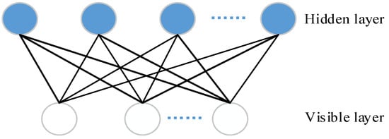 Figure 1. The restricted Boltzmann machine(RBM) model.
The BP network model classifies the features extracted by RBM, and returns the wrong information to the RBM network model, fine-tunes the parameters of the RBM network, and optimizes the DBN model. A network model of a two-tier DBN is shown in Figure 2.
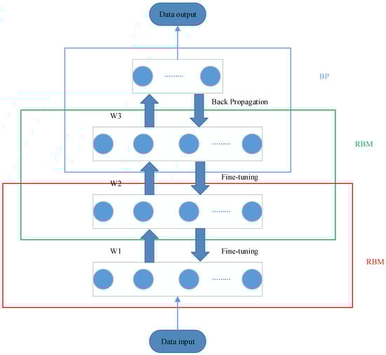
Figure 2.
A network model of a two-tier deep belief network (DBN).
As shown in Figure 2, a two-tier DBN network model figure, that is, after the data is input into the network, they first pass the two RBM layers, and after the output of the RBM layer, they pass through the BP layer, and the result is output after being filtered by the BP layer. On this basis, according to different needs, the RBM layer can continue to join the more layers to construct multi-layer DBN network.
The VMD, mRMR and DBN have been widely applied once they are proposed, so the theory of these methods will not be repeated here. The prediction process of this paper is shown in Figure 3.
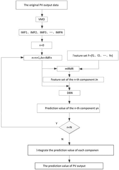
Figure 3.
Theprediction flow figure.
It can be clearly seen from Figure 3 that the photovoltaic output will obtain IMFs with different fluctuation characteristics after being decomposed by VMD, and then mRMR will be used to select the component feature set corresponding to each modal component from the feature set consisting of meteorological factors and photovoltaic output historical values. After obtaining these component feature sets, the component feature sets and their corresponding components are simultaneously input into the DBN for prediction. Finally, the prediction values of each components are integrated using DBN to obtain the final photovoltaic output prediction value.
In this paper, after obtaining the final photovoltaic output prediction value, the average absolute error (MAE), root mean square error (RMSE) and Theil inequality coefficient (TIC) will be used as the three performance evaluation indicators of the prediction model. The calculation formula is as follows:
where represents the total number of samples, represents the actual value, and represents the predicted value. The Theil inequality coefficient is always between 0 and 1, the smaller the value, the smaller the difference between the fitted value and the true value, and the higher the prediction accuracy.
3. Case Study
In this paper, MATLAB is used as the operating environment, and the model proposed in this paper is validated by using the data in 2013 of certain photovoltaic power stations in Yunnan Province of China and certain photovoltaic power station in Gansu Province in China, two provinces that have a large difference between latitudes and altitudes. Both Yunnan and Gansu photovoltaic power stations are equipped with monocrystalline silicon photovoltaic cells. The data of Yunnan photovoltaic power station is an instantaneous value per 15 min, with 96 data points per day. The data of Gansu photovoltaic power station is an instantaneous value every 10 min, and there are 144 data points in a day. The data includes the photovoltaic output, time, temperature and irradiance of the power station. In the prediction process, data, from 2 January 2013 to 23 December 2013, was used to establish the model, and then conducted the prediction on the data from 24 December 2013 to 30 December 2013. In addition, other data such as time, temperature, etc. in the data are used to establish the feature matrix .
3.1. Analysis and Decomposing the Photovoltaic Output
In order to facilitate the observation of photovoltaic data in the two regions, this paper shows the photovoltaic output changes in the two regions in Figure 4.

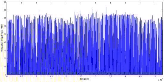
Figure 4.
Thephotovoltaic output map in each region.
It can be seen from Figure 4 that the volatility of the photovoltaic power station output in the two regions is very strong, and the output of Gansu photovoltaic power station is higher than that of Yunnan photovoltaic power station. In order to better observe the photovoltaic output situation in the two regions, the monthly data of two regions is counted, and the statistical results are shown in the Table 1.

Table 1.
Monthly statistics situation of photovoltaic power stations in two regions.
It can be seen from the maximum value of Table 1 that the maximum output of Gansu photovoltaic power station is higher than that of Yunnan photovoltaic power station. In addition, by observing the average and standard deviation of the two power stations, it can be found that the difference between the average value and the standard deviation is larger. From this, it can be seen that the fluctuation of photovoltaic power output of the two power stations is very strong.
In the following analysis, this paper takes Yunnan photovoltaic power station as an example for specific explanation. First, the VMD is used to decompose the photovoltaic output data. The parameter setting in the decomposition process references to [34]. The decomposition results are shown in Figure 5.
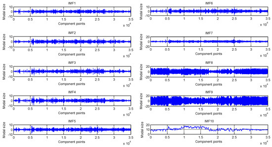
Figure 5.
The image after being decomposed by VMD.
Figure 5 shows each component of photovoltaic output after VMD decomposition. By observing Figure 5, it can be seen that the amplitude fluctuations and frequency fluctuations of the Intrinsic Mode Function (IMF)1~IMF7 components are relatively intense and there is no periodicity, the frequency fluctuation of IMF8~IMF9 is less moderate than the former, but the amplitude fluctuation is much lower, and both the amplitude and frequency fluctuations of the IMF10 are the slowest.
3.2. Establish Feature Sets of Each Component
Photovoltaic output is affected by factors such as season, time, ambient temperature and solar irradiance. After the photovoltaic output is decomposed by VMD, each component contains the effects of the above factors of a different degree. Therefore, this section will study the effect of various factors on each component.
Before establishing each component feature set, an original feature set is established firstly, includes time , season , ambient temperature , solar irradiance , and photovoltaic output history value . Among them, since the photovoltaic data takes a value every 15 min, the time is expressed as 0.0, 0.15, 0.30, 0.45, 1.0, …, 23.30, 23.45. In addition, the season includes spring, summer, autumn and winter, which are represented by numbers 1, 2, 3, and 4 respectively; the photovoltaic output history value represents the photovoltaic historical value before minutes. In addition, the temperature of the photovoltaic panel is not considered in this paper because there are many solar panels in the photovoltaic power station, and the temperature of each photovoltaic panel is different due to the influence of factors such as the angle of illumination, so it is impossible to establish a characteristic factor uniformly.
After the f is established, the mRMR is used to establish the feature set of each component. The specific process is shown in Figure 6.

Figure 6.
The flow chart of feature selection of components.
In Figure 6, is the number of components after VMD decomposition. As can be seen from Figure 6, the selection step of the component feature set is as follows:
- Use an incremental search method to establish a candidate feature set of the component;
- Calculate the mRMR values of each feature in and arrange them in descending order according to the magnitude of the mRMR value, and then input them into error function one by one to obtain the error;
- Take the number of features corresponding to the minimum error to establish a component feature set.
The error function in Figure 6 uses the root mean square error (RMSE), which is calculated as shown in Equation (2). The errors obtained by inputting the feature factors, which is ordered in descending order according to the mRMR, of each component into the error function one by one are shown in Table 2.
Table 2.
The errors obtained by inputting the feature factors of each component into the error function one by one.
The letters in the Table 2 represent the names of each feature, the numbers are the error values, and the red numbers represent the smallest errors. The names of the features in the table are cumulative, for example, the of IMF1 means that the error value obtained by inputting and its previous together into the error function is 0.0254. By observing Table 2, it can be seen that except for IMF8, for other component features, are all ranked the front, it can be seen that time has the greatest influence on the component, and it can be concluded that the photovoltaic output is greatly affected by the alternating day and night in one day, only in the daytime can a photovoltaic power station generate electricity and it cannot generate electricity at night. In addition, the effects of the irradiance intensity and the temperature on each component are also large. In comparison, the photovoltaic historical value seems to have a weak influence on each component.
From Table 2 and the above discussion, it is found that the feature set of each component is as shown in Table 3.
Table 3.
The feature set of each component.
By observing Table 3, it can be clearly seen that the components containing the feature are IMF1~IMF7 and IMF9~IMF10; the components containing the stochastic features as or are IMF1~IMF6 and IMF9~IMF10; the components containing the feature are IMF3, IMF6 and IMF10. It can be seen that most of the components are affected by day and night alternation and environmental changes, while IMF3, IMF6 and IMF10 also contain information on the impact of seasonal changes on photovoltaic output.
3.3. The Components and Photovoltaic Output Prediction
After obtaining the feature set of each component, each component is input into the DBN along with its corresponding feature set to conduct the prediction. When training the DBN network, a 3-input 1-output model is used, that is, three points of each component and three points of the corresponding features are input together. The number of hidden layers in the parameter setting process and the number of units in each hidden layer references to [35], and other parameters setting uses reference [36]. Then, the DBN structure of each component is as shown in Table 4.
Table 4.
The DBN structure of each component.
After obtaining the structure of each component prediction model, components with various frequencies are predicted using the model trained well, and the prediction result is shown in Figure 7.

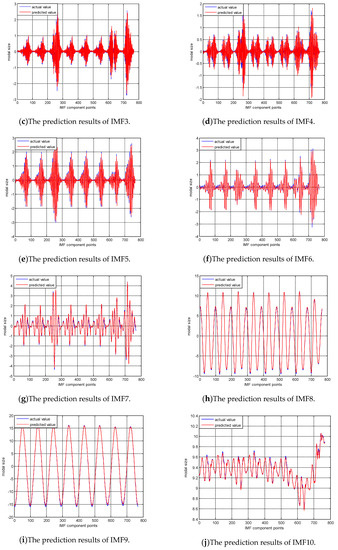
Figure 7.
The prediction image of components with various frequency.
Combining Figure 7 and the corresponding RMSE error in Table 2, it can be seen that from IMF1 to IMF10, as the component fluctuations weaken, the error begins to decrease, especially after IMF7, the error is relatively small. But overall, the prediction results of each component are ideal.
After the prediction of each component is completed, the DBN is used to integrate the prediction results of each component. Taking the actual value of each component as input and taking the actual photovoltaic output value as output fortraining the model, the prediction values of the components are taken as inputs, and using the model trained well to obtain the photovoltaic prediction values. The prediction results are shown in Figure 8.
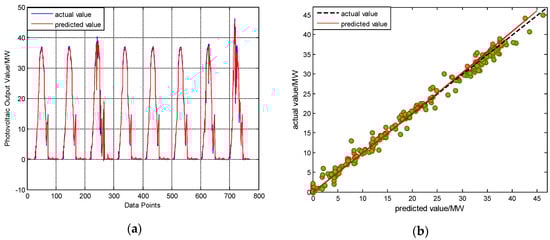
Figure 8.
The prediction results of photovoltaic output. (a) Predicted and observed values; (b) Fitting Chart of Prediction Result.
The left half of Figure 8 is the result plot of the prediction and actual values, and the right half is the comparison of the actual value with the prediction value; the green point in the figure is the distribution point of the prediction value. It can be seen from Figure 8 that compared with the error of other intervals, except for the interval 35–40 has the larger error; in the other intervals, the actual value and the prediction value are very close, and most of the green points distribute near the actual value.
3.4. The Comparison
For more intuitive comparative analysis, this paper uses the MAE, MSE, and RMSE mentioned above to compare the prediction results of this paper with that of the Auto-Regressive Moving Average Model (ARMA) and DBN single prediction model and the EMD, EEMD, and VMD decomposition combined prediction models. For the single prediction model, the original photovoltaic output data are directly used for modeling and prediction; for the decomposition combined prediction model, the original photovoltaic output data are first decomposed using EMD, EEMD and VMD, and then each frequency component is predicted using DBN, and finally the prediction results of each frequency component are integrated to obtain a final prediction photovoltaic output value. For the comparison results of the models, the comparison results of Yunnan photovoltaic power station data are shown in Table 5, and the comparison results of Gansu photovoltaic power station data are shown in Table 6.
Table 5.
The comparison results of Yunnan photovoltaic power station.
Table 6.
The comparison results of Gansu photovoltaic power station.
It can be seen from Table 5 that the prediction accuracy of the decomposition-combined prediction model is better than that of the single prediction model. For example, for the MAE of EMD decomposition-combined prediction model improved by 50.2% compared with the ARMA, and by 41.3% compared with the DBN; for the MAE of EEMD decomposition-combined prediction model improved by 62.9% compared with the ARMA, and by 56.3% compared with the DBN; and for the MAE of VMD decomposition-combined prediction model improved by 78.3% compared with the ARMA, and by 74.4% compared with the DBN. In the decomposition-combined prediction model, the VMD decomposition-combined model has higher prediction accuracy than the EEMD and EMD decomposition-combined model. For example, for the RMSE, the prediction accuracy of VMD combined decomposition model respectively improved by 45.8% and 55% compared with the EEMD decomposition-combined model and the EMD decomposition-combined model. It can be seen that after using VMD to decompose the photovoltaic output, the prediction accuracy is greatly improved. After considering the influence of the characteristic factors, the prediction accuracy is further improved. It can be seen from Table 4 that for MAE, RMSE and TIC, the prediction model of this paper improved respectively by 60.0%, 35.4% and 42.4% compared with the VMD decomposition-combined model. It can be seen that for the Yunnan photovoltaic power station data, the prediction accuracy of model in this paper is higher.
It can also be seen from Table 6 that the accuracy of the decomposition-combined prediction model is better than that of the single prediction model, while the prediction model of this paper has higher prediction accuracy than other decomposition-combined prediction models; for example, the MAE of this paper improved by 58.0% compared with the VMD decomposition-combined prediction model, and by 74.1% compared with the EEMD decomposition-combined prediction model, by 79.9% compared with the EMD decomposition-combined model, by 90.1% compared with the DBN model, and by 91.6% compared with the ARMA model.
Based on the comparison of the prediction results of the above two photovoltaic power station, it can be seen that after using the VMD to decompose the photovoltaic output data into modal components with different wave characteristics and using mRMR to analyze the influence of each influencing factor on each frequency component, the prediction accuracy of this paper exceeds that of the traditional decomposition-combined prediction model and the single prediction model. In addition, this paper uses the rolling prediction method in the prediction process, that is, the actual value is continuously absorbed into the model during the prediction process. For example, at moment , after finishing predicting the value at moment , the true value of the moment and the corresponding influence component are added to the model to predict the value at the next moment. Therefore, this paper can make real-time continuous prediction of photovoltaic output.
4. Conclusions
In order to make full use of the random and intermittent photovoltaic output, this paper uses VMD to decompose the photovoltaic output and obtains the modal components with different fluctuation characteristics. The photovoltaic output is affected by solar irradiance, ambient temperature, etc., and this paper uses mRMR to conduct the feature selection on each component. In the process of selection, a raw feature matrix consisting of time, temperature, season, irradiance intensity and photovoltaic output historical values is firstly established. Then we determine the candidate feature set of each component using the incremental search method and sort the features in the candidate feature set in descending mRMR value order. Finally, input the features after ordering one by one into the error function to select the number of features with the smallest error as the component feature set. After obtaining each component feature set, these are input into the DBN for component prediction together with the corresponding components. Finally, prediction results of each component are integrated to obtain the final photovoltaic output prediction result, and compared with other models, and it is found that the prediction accuracy of the model in this paper is higher.
When establishing a candidate feature set of each component, it is found that the incremental search method is cumbersome, and then the mRMR values of the features selected by using the method need to be sorted in descending order. Therefore, it is somewhat redundant to use the incremental search method to determine the candidate feature set, so whether there is a simpler and more direct method to select the candidate feature set of each component will be our next research direction.
Author Contributions
P.D. and G.Z. conceived and designed the experiments; P.D. and H.L. performed the experiments; P.L. and M.L. analyzed the data; P.D. and J.H. contributed reagents/materials/analysis tools; P.D. wrote the paper.
Funding
This work was Supported by the National Key Research and Development Program of China, (Grant No. 2016YFC0401409), and the National Natural Science Foundation of China,(Grant No. 51679186, Grant No. 51679188, Grant No. 51979221, Grant No. 51709222), and the Research Fund of the State Key Laboratory of Eco-hydraulics in Northwest Arid Region, Xi’an University of Technology, (Grant No. 2019KJCXTD-5), and the Key Research and Development Plan of Shaanxi Province, (Grant No. 2018-ZDCXL-GY-10-04), and the Natural Science Basic Research Program of Shaanxi (Program No. 2019JLZ-15). Sincere gratitude is extended to the editor and anonymous reviewers for their professional comments and corrections.
Conflicts of Interest
The authors declare no conflict of interest.
References
- Liu, J.P.; Long, Y.; Song, X.H. A Study on the Conduction Mechanism and Evaluation of the Comprehensive Efficiency of Photovoltaic Power Generation in China. Energies 2017, 10, 22. [Google Scholar]
- Sen, S.; Ganguly, S. Opportunities, barriers and issues with renewable energy development—A discussion. Renew. Sust. Energ. Rev. 2017, 69, 1170–1181. [Google Scholar] [CrossRef]
- Zang, H.; Cheng, L.; Ding, T.; Cheung, K.W.; Liang, Z.; Wei, Z.; Sun, G. Hybrid method for short-term photovoltaic power forecasting based on deep convolutional neural network. IET Gener. Transm. Distrib. 2018, 12, 4557–4567. [Google Scholar] [CrossRef]
- Voyant, C.; Motte, F.; Fouilloy, A.; Notton, G.; Paoli, C.; Nivet, M.-L. Forecasting method for global radiation time series without training phase: Comparison with other well-known prediction methodologies. Energy 2017, 120, 199–208. [Google Scholar] [CrossRef]
- Watanabe, T.; Nohara, D. Prediction of time series for several hours of surface solar irradiance using one-granule cloud property data from satellite observations. Sol. Energy 2019, 186, 113–125. [Google Scholar] [CrossRef]
- Chantana, J.; Kawano, Y.; Kamei, A.; Minemoto, T. Description of degradation of output performance for photovoltaic modules by multiple regression analysis based on environmental factors. Optik 2019, 179, 1063–1070. [Google Scholar] [CrossRef]
- Li, Y.; Wang, Z.; Niu, J. Forecast of power generation for grid-connected photovoltaic system based on grey theory and verification model. In Proceedings of the Fourth International Conference on Intelligent Control and Information Processing, Beijing, China, 9–11 June 2013; pp. 129–133. [Google Scholar]
- Persson, C.; Bacher, P.; Shiga, T.; Madsen, H. Multi-site solar power forecasting using gradient boosted regression trees. Sol. Energy 2017, 150, 423–436. [Google Scholar] [CrossRef]
- Yang, C.; Thatte, A.A.; Xie, L. Multitime-Scale Data-Driven Spatio Temporal Forecast of Photovoltaic Generation. IEEE Trans. Sustain. Energy 2015, 6, 104–112. [Google Scholar] [CrossRef]
- Guan, L.; Zhao, Q.; Zhou, B.; Lyu, Y.; Zhao, W.; Yao, W. Multi-scale Clustering Analysis Based Modeling of Photovoltaic Power Characteristics and Its Application in Prediction. Autom. Electr. Power Syst. 2018, 42, 24–30. [Google Scholar]
- Wang, Y.; Fu, Y.; Sun, L.; Xue, H. Ultra-Short Term Prediction Model of Photovoltaic Output Power Based on Chaos-RBF Neural Network. Power Syst. Technol. 2018, 42, 1110–1116. [Google Scholar]
- Andrews, R.W.; Pearce, J.M. Prediction of energy effects on photovoltaic systems due to snow fall events. In Proceedings of the 38th IEEE Photovoltaic Specialists Conference, Austin, TX, USA, 3–8 June 2012; pp. 3386–3391. [Google Scholar]
- Long, H.; Zhang, Z.; Su, Y. Analysis of daily solar power prediction with data-driven approaches. Appl. Energy 2014, 126, 29–37. [Google Scholar] [CrossRef]
- Gao, Y.; Zhu, J.; Cheng, H.; Xue, F.; Xie, Q.; Li, P. Study of Short-Term Photovoltaic Power Forecast Based on Error Calibration under Typical Climate Categories. Energies 2016, 9, 523. [Google Scholar] [CrossRef]
- Zhu, Y.; Tian, J. Application of Least square Support Vector Machine in Photovoltaic Power Forecasting. Power Syst. Technol. 2011, 35, 54–59. [Google Scholar]
- Mittal, M.; Bora, B.; Saxena, S.; Gaur, A.M. Performance prediction of PV module using electrical equivalent model and artificial neural network. Sol. Energy 2018, 176, 104–117. [Google Scholar] [CrossRef]
- Ding, M.; Xu, N. A Method to Forecast Short-Term Output Power of Photovoltaic Generation System Based on Markov Chain. Power Syst. Technol. 2011, 35, 152–157. [Google Scholar]
- Eseye, A.T.; Zhang, J.; Zheng, D. Short-term photovoltaic solar power forecasting using a hybrid Wavelet-PSO-SVM model based on SCADA and Meteorological information. Renew. Energy 2018, 118, 357–367. [Google Scholar] [CrossRef]
- Marquez, R.; Coimbra, C.F.M. Forecasting of global and direct solar irradiance using stochastic learning methods, ground experiments and the NWS database. Sol. Energy 2011, 85, 746–756. [Google Scholar] [CrossRef]
- Li, J.; Huang, Q.; Wei, S.; Huang, Y. Improved Deep Learning Algorithm Based on S-BGD and Gradient Pile Strategy and Its Application in PV Power Forecasting. Power Syst. Technol. 2017, 41, 3292–3300. [Google Scholar]
- Malvoni, M.; DeGiorgi, M.G.; Congedo, P.M. Photovoltaic forecast based on hybrid PCA-LSSVM using dimensionality reducted data. Neurocomputing 2016, 211, 72–83. [Google Scholar] [CrossRef]
- Li, F.-F.; Wang, S.-Y.; Wei, J.-H. Long term rolling prediction model for solar radiation combining empirical mode decomposition (EMD) and artificial neural network (ANN) techniques. J. Renew. Sustain. Energy 2018, 10, 013704. [Google Scholar] [CrossRef]
- Wang, H.; Sun, J.; Wang, W. Photovoltaic Power Forecasting Based on EEMD and a Variable-Weight Combination Forecasting Model. Sustainability 2018, 10, 2627. [Google Scholar] [CrossRef]
- Mao, M.; Gong, W.; Chang, L.; Cao, Y.; Xu, H. Short-term Photovoltaic Generation Forecasting Based on EEMD-SVM Combined Method. Proc. Chin. Soc. Electr. Eng. 2013, 33, 17–24. [Google Scholar]
- Xie, T.; Zhang, G.; Liu, H.; Liu, F.; Du, P. A Hybrid Forecasting Method for Solar Output Power Based on Variational Mode Decomposition, Deep Belief Network sand Auto-Regressive Moving Average. Appl. Sci. 2018, 8, 1901. [Google Scholar] [CrossRef]
- He, X.; Luo, J.; Zuo, G.; Xie, J. Daily Run off Forecasting Using a Hybrid Model Based on Variational Mode Decomposition and Deep Neural Networks. Water Resour. Manag. 2019, 33, 1571–1590. [Google Scholar] [CrossRef]
- Xie, T.; Zhang, G.; Hou, J.; Xie, J.; Lv, M.; Liu, F. Hybrid forecasting model for non-stationary daily run off series: A case study in the Han River Basin, China. J. Hydrol. 2019, 577, 123915. [Google Scholar] [CrossRef]
- Han, Y.; Wang, N.; Ma, M.; Zhou, H.; Dai, S.; Zhu, H. A PV power interval forecasting based on seasonal model and nonparametric estimation algorithm. Sol. Energy 2019, 184, 515–526. [Google Scholar] [CrossRef]
- Kim, G.G.; Choi, J.H.; Park, S.Y.; Bhang, B.G.; Nam, W.J.; Cha, H.L.; Park, N.; Ahn, H.-K. Prediction Model for PV Performance with Correlation Analysis of Environmental Variables. IEEE J. Photovolt. 2019, 9, 832–841. [Google Scholar] [CrossRef]
- Liu, J.; Sun, H.; Chang, P.; Jiao, Z.; Wei, P.; Ke, X.; Sun, X.; Cheng, L. Research of Photovoltaic Power Forecasting Based on Big Data and mRMR Feature Reduction. In Proceedings of the2018 IEEE Power & Energy Society General Meeting, Portland, OR, USA, 5–9 August 2018. [Google Scholar]
- Dragomiretskiy, K.; Zosso, D. Variational Mode Decomposition. IEEE Trans. Signal Process. 2014, 62, 531–544. [Google Scholar] [CrossRef]
- Peng, H.; Long, F.; Ding, C. Feature selection based on mutual information: Criteria of Max-Dependency, Max-Relevance, and Min-Redundancy. IEEE Trans. Pattern Anal. Mach. Intell. 2005, 27, 1226–1238. [Google Scholar] [CrossRef]
- Hinton, G.; Deng, L.; Yu, D.; Dahl, G.E.; Mohamed, A.-R.; Jaitly, N.; Senior, A.; Vanhoucke, V.; Patrick, N.; Sainath, T.N.; et al. Deep Neural Networks for A coustic Modeling in Speech Recognition. IEEE Signal Process. Mag. 2012, 29, 82–97. [Google Scholar] [CrossRef]
- Cui, J.; Yu, R.; Zhao, D.; Yang, J.; Ge, W.; Zhou, X. Intelligent load pattern modeling and denoising using improved variational mode decomposition for various calendar periods. Appl. Energy 2019, 247, 480–491. [Google Scholar] [CrossRef]
- Alshamaa, D.; Chehade, F.M.; Honeine, P. A hierarchical classification method using belief functions. Signal Process. 2018, 148, 68–77. [Google Scholar] [CrossRef]
- Fu, G. Deep belief network based ensemble approach for cooling load forecasting of air-conditioning system. Energy 2018, 148, 269–282. [Google Scholar] [CrossRef]


© 2019 by the authors. Licensee MDPI, Basel, Switzerland. This article is an open access article distributed under the terms and conditions of the Creative Commons Attribution (CC BY) license (http://creativecommons.org/licenses/by/4.0/).