Study into the Improvement of Dynamic Stress Characteristics and Prototype Test of an Impeller Blade of an Axial-Flow Pump Based on Bidirectional Fluid–Structure Interaction

Featured Application

The thickness of rotating parts of hydraulic machineries, such as the impeller blade of axial pump studied in this paper, affect the hydraulic performance as known. However, unsuitable thin thickness will cause cracks on the structure. This paper design and validate an approach of thickening impeller blade root to increase the strength of blade and minimize the impact on hydraulic performance. An experimental method for the underwater measurement of the dynamic stress of prototypical hydraulic machinery was put forward to validate the simulation results. This study can be referred to enhance stability at design stage for structure of hydraulic machineries’ blades.

Abstract

This paper performed a numerical study into the dynamic stress improvement of an axial-flow pump and validated the simulation results with a prototype test. To further analyze the dynamic stress characteristics of impeller blades of axial-flow pumps, a bidirectional fluid–structure interaction (FSI) was applied to numerical simulations of the unsteady three-dimensional (3-D) flow field of the whole flow system of an axial-flow pump, and the gravity effect was also taken into account. In addition, real-structure-based single-blade finite element model was established. By using the finite element method, a calculation of the blade’s dynamic characteristics was conducted, and its dynamic stress distribution was determined based on the fourth strength theory. The numerical results were consistent with the prototype tests. In a rotation cycle, the dynamic stress of the blade showed a tendency of first increasing, and then decreasing, where the maximum value appeared in the third quadrant and the minimum appeared in the first quadrant in view of the gravity effect. A method for reducing the stress concentration near the root of impeller blades was presented, which would effectively alleviate the possibility of cracking in the unreliable region of blades. Simultaneously, an experimental method for the underwater measurement of the dynamic stress of prototypical hydraulic machinery was put forward, which could realize the underwater sealing of data acquisition instruments on rotating machinery and the offline collection of measured data, finally effectively measuring the stress of underwater moving objects.

1. Introduction

Pump station engineering guarantees the optimal allocation and scheduling of water resources. As an important underwater rotating component of a pump unit, the impeller is the most vulnerable structure among all structural components during actual operation. Cracks and even ruptures of the blades are not rare in numerous pump and hydropower stations around the world and severely threaten the safe and stable operation of pump units. Thus, the study of the structural characteristics of pump units is urgently required.

With the development of fluid–structure interaction (FSI) computational techniques, plenty of studies have emerged with regard to the finite element analysis of structural characteristics of hydraulic machinery. Schneider et al. [1] studied the stress and deformation characteristics of a multiple-stage centrifugal pump with the effect of structural parameters and temperature through one-way coupled FSI. The results showed that the deformation and the stress distributions vary significantly with the operating point, and cases in hot fluid conditions are more critical. Trivedi [2] analyzed the hydrodynamic damping in hydraulic turbines, which is found to be dependent on the nodal diameter of the mode shape, and the damping effect is proportional to the free-stream flow velocity. Kan et al. [3] conducted a structural static analysis on a Francis turbine runner; under different water heads and openings of the guide vanes, the rules of the equivalent stress and deformation of the runner were obtained and analyzed. Pei et al. [4] calculated the impeller dynamic stress of a single-blade centrifugal sewage pump in different working conditions and obtained the dynamic stress distribution of the impeller rotor system by using bidirectional FSI. On the basis of FSI, Campbell et al. [5] numerically investigated the deformation of impellers in a low-rigidity pump, with the results being consistent with those obtained via experiments in circulating water channels. Langthjem et al. [6] conducted a study into the flow-induced noise of a centrifugal pump in consideration of FSI. Additionally, multiple scholars have studied FSI problems by introducing the immersed boundary method (IBM), which could avoid the numerical instability induced by grid deformation due to FSI [7,8,9,10,11]. Among the current studies on FSI [1,2,3,4,5,6,7,8,9,10,11,12,13,14,15,16,17], few are related to the structural dynamic stress of axial-flow pump impellers, and the structural response to the transient fluid–structure interaction (FSI) of axial-flow pump impellers has not been studied in depth. Meanwhile, the overall structure of an impeller has been selected as the research object for finite element analysis in the majority of studies [13,14,15,16,17], which could not show the performance of a real pump impeller accurately. Furthermore, a great amount of numerical simulations lack comparison and validation, which leads to uncertain reliability. Therefore, this paper aims to study the dynamic stress improvement in depth to enhance the reliability of impellers based on real blade models and to validate the simulation accuracy by comparing the models with the results of a prototype test.

In this paper, a bidirectional FSI study of an impeller blade in the whole flow system of a shaft-extension axial-flow pump is carried out to obtain the distribution of dynamic stress characteristics of impeller blades with different heads. Moreover, a thickening method for the stress state improvement of blade roots and an experimental method to measure the dynamic stress of real underwater rotating machinery are presented, which could give a valuable reference in respect to theoretical design and engineering applications.

2. Theory of Computing Methods

2.1. Computing Method of Flow Fields

According to the continuity equation and the Navier–Stokes equation, the internal flow of fluid machinery can be described as follows [18,19,20,21,22]:

The continuity equation is as follows:

$$\frac{\partial {\mathit{u}}_i}{\partial x_i}=0$$

(1)

The Navier–Stokes equation is as follows:

$$\rho \frac{\partial {\mathit{u}}_i}{\partial x_i}+\rho {\mathit{u}}_j\frac{\partial {\mathit{u}}_i}{\partial x_j}=\rho {\mathit{f}}_i-\frac{\partial p}{\partial x_i}+\mu \frac{{\partial }^2{\mathit{u}}_i}{\partial x_i\partial x_j}$$

(2)

where u refers to the fluid velocity vector, ρ means the fluid density, f_i is mass force, p stands for pressure, μ is dynamic viscosity, and x_i and x_j refer to position vectors, respectively.

In the flow of pumps, the flow near the boundary layer cannot be forecasted correctly by wall functions when boundary-layer separation occurs around blades. In this condition, the automatic wall treatment model based on k-ω equations is embedded into a wall equation with a low Reynolds number in the near-wall region, which contributes to the avoidance of excessive predictions for eddy viscosity. Thus, in this paper, the shear-stress transport (SST) k-ω turbulence model [17,23,24,25,26,27,28] is selected to simulate the flow characteristics of flow fields.

2.2. Computing Method of Structure Fields

The finite element equation for the calculation of structure is described in [29,30]:

$$\mathit{M}{\ddot{\mathit{q}}}_t(t)+C{\dot{\mathit{q}}}_t(t)+\mathit{K}{\mathit{q}}_t(t)=\mathit{Q}(t)$$

(3)

where M stands for the matrix of structure mass, C means the matrix of structural damping, K refers to the matrix of structural rigidity, Q(t) is the fluid load vector, ${\ddot{\mathit{q}}}_t(t)$ is the node acceleration vector, ${\dot{\mathit{q}}}_t(t)$ refers to the node velocity vector, and ${\mathit{q}}_t(t)$ is the node displacement vector.

According to the fourth strength theory, the equivalent stress can be written as follows [31]:

$${\sigma }_e=\sqrt{\frac{1}{2}\left[{\left({\sigma }_1-{\sigma }_2\right)}^2+{\left({\sigma }_2-{\sigma }_3\right)}^2+{\left({\sigma }_3-{\sigma }_1\right)}^2\right]}$$

(4)

where σ₁, σ₂, and σ₃ refer to three principal stresses.

2.3. Theory of Stress Measurement

As the resistance of a metal wire changes with its deformation—namely the resistance strain effect—strain gauges have been invented. When the stress–strain of a test piece is measured with a resistance strain gauge, the deformation of the test piece is detected by the output of electrical signals with the gauge attached to the test piece. The relation of some parameters of the metal wire is described by

$$R=\lambda \frac{L}{A}$$

(5)

where R is the resistance of a metal wire, L is the length of a metal wire, A is the cross-sectional area of a metal wire, and λ is the electrical resistivity.

When the test piece deforms, its resistance changes accordingly. The variation can be solved through the differential form of Equation (5):

$$\frac{dR}{R}=\frac{d\lambda }{\lambda }+\frac{dL}{L}-\frac{dA}{A}$$

(6)

where $\frac{dL}{L}=\epsilon$ corresponds to the strain, and $\frac{dA}{A}$ refers to the relative variation of the cross-sectional area of a metal wire, which can be calculated by $\frac{dA}{A}=-2\tau \frac{dL}{L}=-2\tau \epsilon$ (τ refers to the Poisson’s ratio of a wire) for both circular and rectangular cross-sections. Substituting this relation into Equation (6), we obtain the following:

$$\frac{dR}{R}=\left(1+2\tau \right)\frac{dL}{L}+\frac{d\lambda }{\lambda }=\left(1+2\tau \right)\epsilon +\frac{d\lambda }{\lambda }$$

(7)

In addition, according to the material characteristics:

$$\frac{d\rho }{\rho }=C\frac{dV}{V}=C\left(1-2\mu \right)\frac{dL}{L}$$

(8)

where V = A × L indicates the volume of a wire. The coefficient C depends on the proportionality coefficient of the crystal structure of metal conductors. For common metals and alloys, C ranges from −12 (nickel) to +6 (platinum). Substituting Equation (8) into Equation (7):

$$\frac{dR}{R}=\left[1+2\tau +C\left(1-2\tau \right)\right]\epsilon =K_0\epsilon$$

(9)

where K₀ refers to the sensitivity coefficient of a wire, namely the relative variation of resistance caused by unit strain.

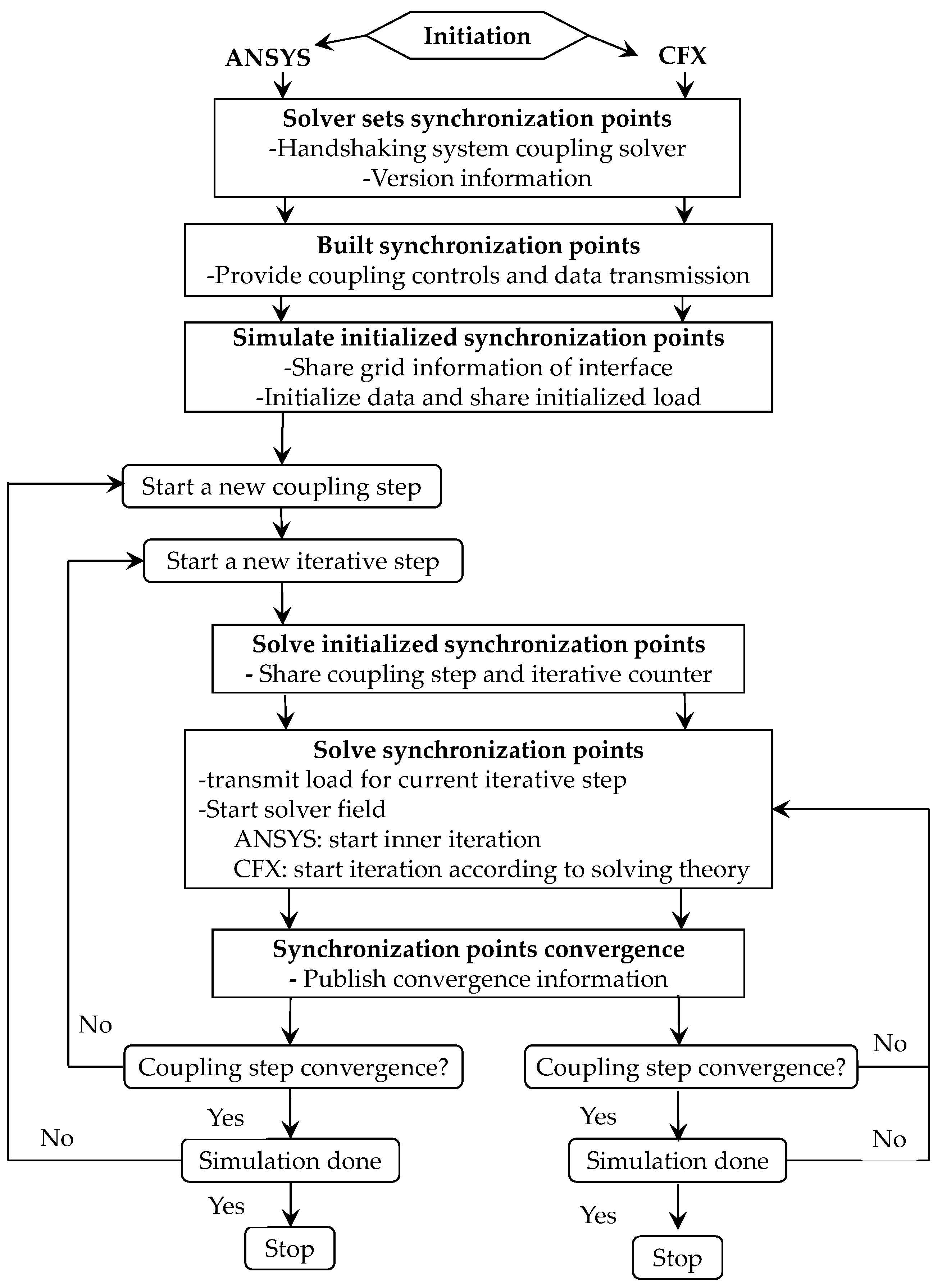
2.4. Patterns of Data Transmission

In view of the interaction between the impeller structure and flow fields, bidirectional FSI was applied to the simulations. Here, data are transferred between computational fluid X (CFX) and the structure analysis module on an interface through the ANSYS multi-field Solver (MFS). The flow field pressure distribution in the whole flow system of the axial-flow pump are obtained by CFX, and then the pressure values on the blade are delivered to the structure analysis module to solve the displacement and deformation. The corresponding feedback of deformation on the flow field can be updated again through CFX. The moment of data exchange between flow fields and structure fields is called the synchronization point, except for data which cannot be transmitted. Figure 1 shows the fundamental principle.

3. Flow Field Calculation

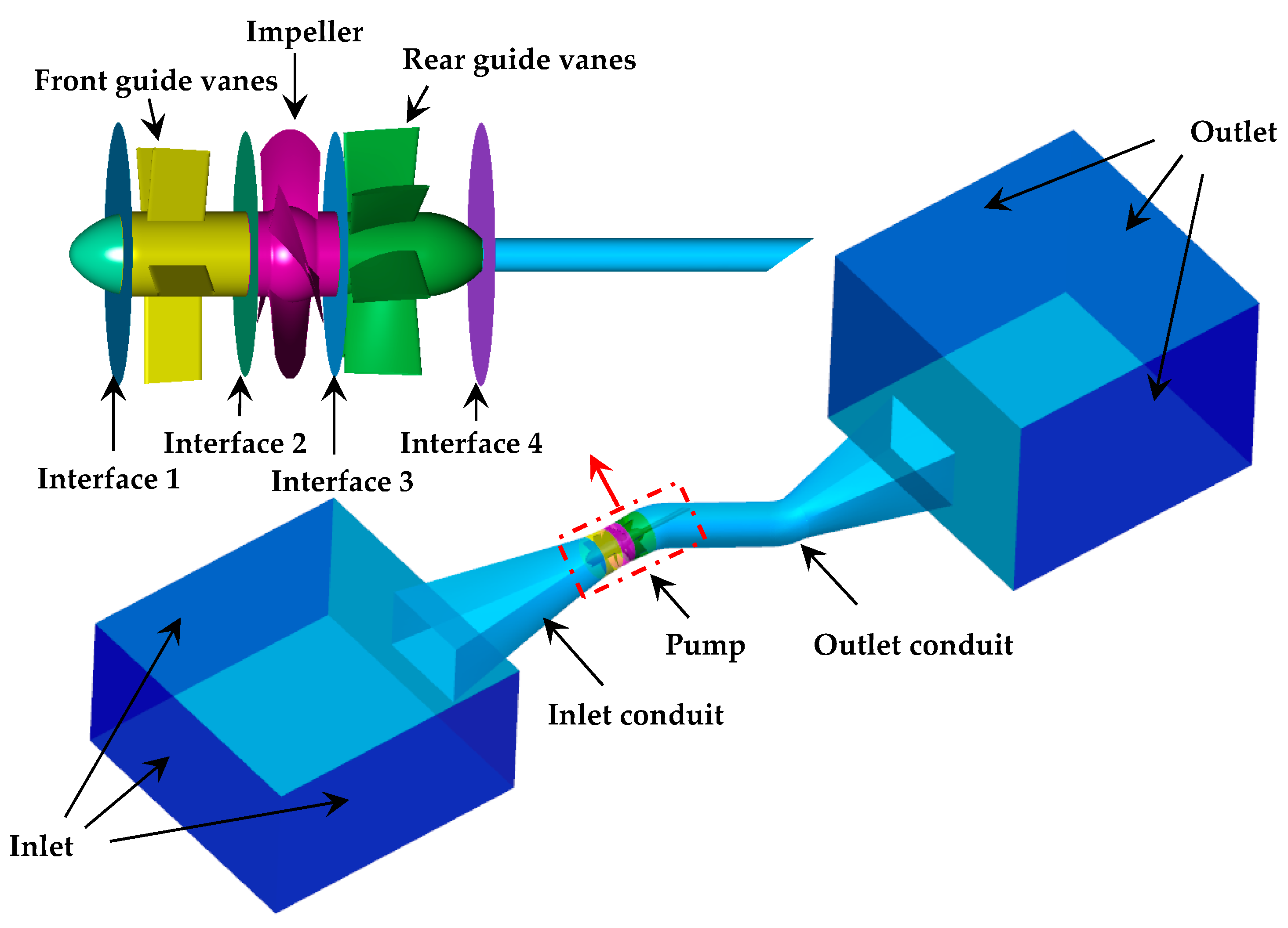
3.1. Calculation of Models and Operating Points

The whole flow system of a shaft-extended axial-flow pump involved in this simulation includes an inlet reservoir, inlet conduit, front guide vanes, impellers, rear guide vanes, outlet conduit and an outlet reservoir, whose detailed structure is displayed in Figure 2 and characteristic parameters are listed in

Table 1. Characteristic parameters of the pump flow system.

Parameters	Value
Diameter of impeller/m	1.7
Number of impeller blades/-	4
Number of inlet guide vanes/-	5
Number of outlet guide vanes/-	7
Blade rated angle/°	−6~4
Design head/m	2.5
Design speed/r/min	250
Design discharge/m3/s	10

. The inlet and outlet conduits are plane “S”-shaped, and the impeller adopts S-shaped blades. In order to comprehensively analyze the dynamic stress characteristics of the impeller blade of pump units, the installing angle of the blades is fixed as 0°, and four different pump heads, namely 2.5 m, 3 m, 3.5 m and 4 m, respectively, are selected for the calculation.

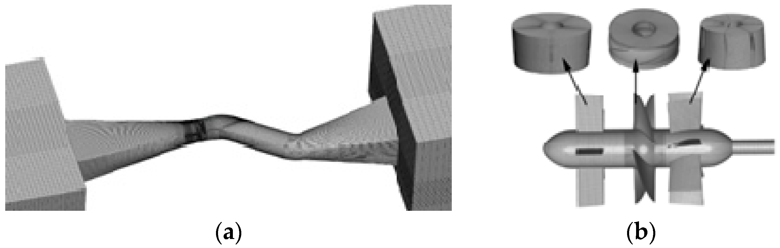
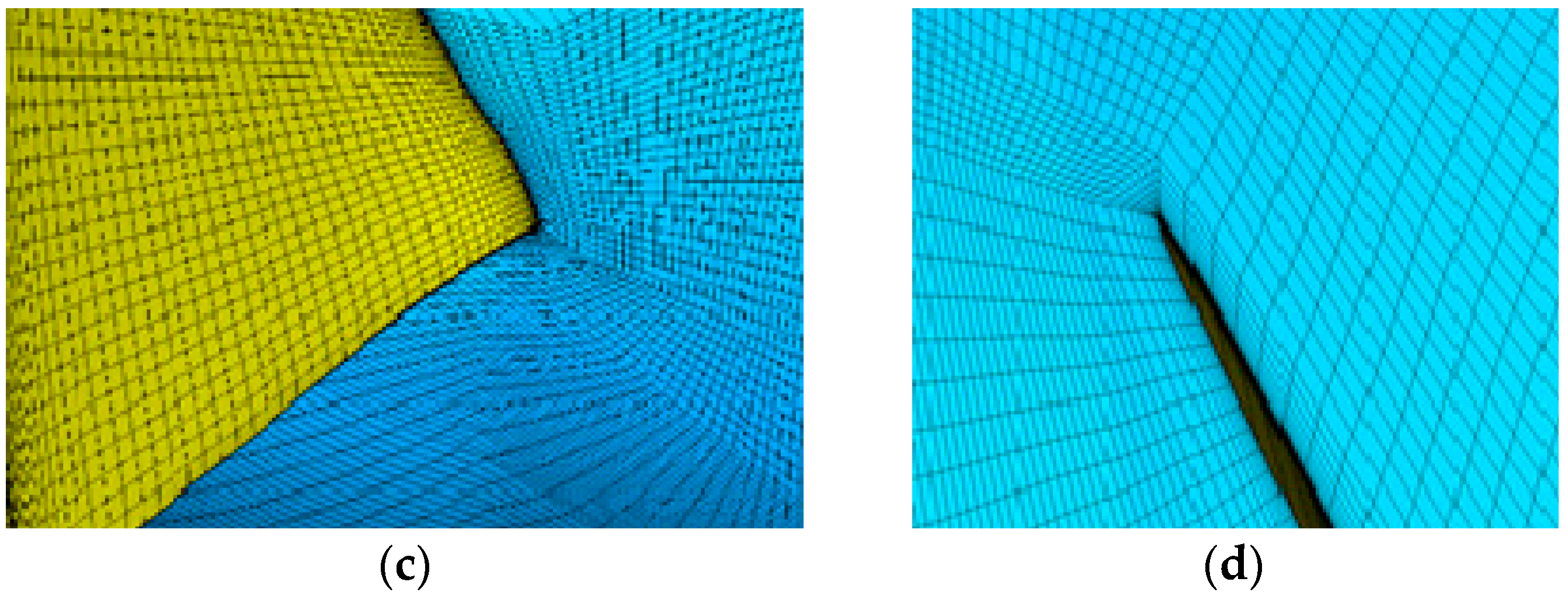
3.2. Grid Partition and Sensitivity Analysis

In the numerical simulation, the quality of grids directly affects the accuracy and efficiency of computation, as well as the validity and reliability of computing results. Thus, a hexahedron-structured grid partition is conducted with the integrated computer engineering and manufacturing code (ICEM) software (ANSYS 15.0 2013, Canonsburg, PA, USA), where an H-shaped grid topology is applied to the front and rear guide vanes. In addition, considering that the wrap angles of impeller blades are large, J-shaped grid topology was applied for impellers. Also, boundary-layer grid division and local refinement near the walls of the overflow components were carried out. A sensitivity analysis of partitioned grids of different sizes was conducted, where 2.31 × 10⁶, 3.24 × 10⁶, 4.21 × 10⁶ and 4.75 × 10⁶ grids were selected. The relative variation ratio of the torque and flow rate was less than 1.7% when the grid number exceeded 4.21 × 10⁶. Therefore, 4.21 × 10⁶ units of grids were chosen for the fluid calculation domain of the whole pump unit, as shown in Figure 3.

3.3. Equation Discretization and Boundary Conditions

The numerical simulation of flow fields was implemented on the CFX platform (ANSYS 15.0 2013, Canonsburg, PA, USA), and the finite volume method (FVM) was applied to discretize the governing equations. A high-order solution was used for the convective term and diffusion term, and pressure gradients were expressed by finite element functions. Fully-implicit multi-grid coupling was utilized for the solution of flow fields by coupling momentum equations and the continuity equation [21,25]. In view of the gravity effects on the overall flow fields, the pressure inlet and outlet along water depths and different operating conditions were set up by the CFX expression language (CEL). Adiabatic and no-slip boundary conditions were adopted for the solid walls. The junction of the impeller fluid domain and solid impeller was defined as the FSI boundary. The transient frozen rotor method was conducted to transmit information between dynamic and static regions with a time step of 0.001 s; i.e., a blade rotates 1.5° in each time step, and there are 240 time steps in each cycle. Considering the computational economic efficiency and reliability, eight complete cycles were applied to the overall stimulation, and then the total physical time was 1.92 s.

3.4. Comparison of Flow Fields

To verify the accuracy and reliability of the numerical simulation, some characteristic parameters—i.e., flow rate Q, head H and efficiency η—are compared with prototype experimental data in Figure 4. The calculated values of Q, H and η were in good accordance with the test values within a 3% error, which verifies that the numerical calculation models and methods applied in this paper could truly reflect the characteristics of this axial-flow pump. The following study on the dynamic stress characteristics of axial-flow pumps can be forecasted accurately.

4. Calculation of Structure Stress Fields

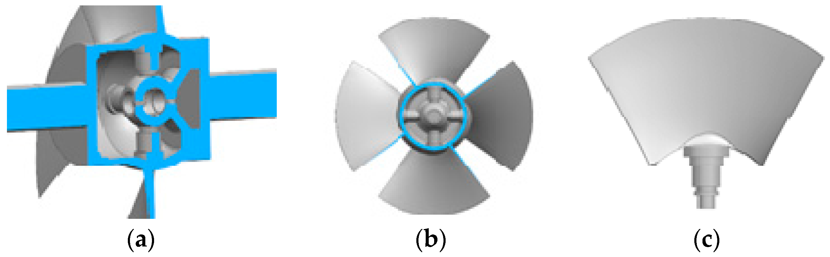
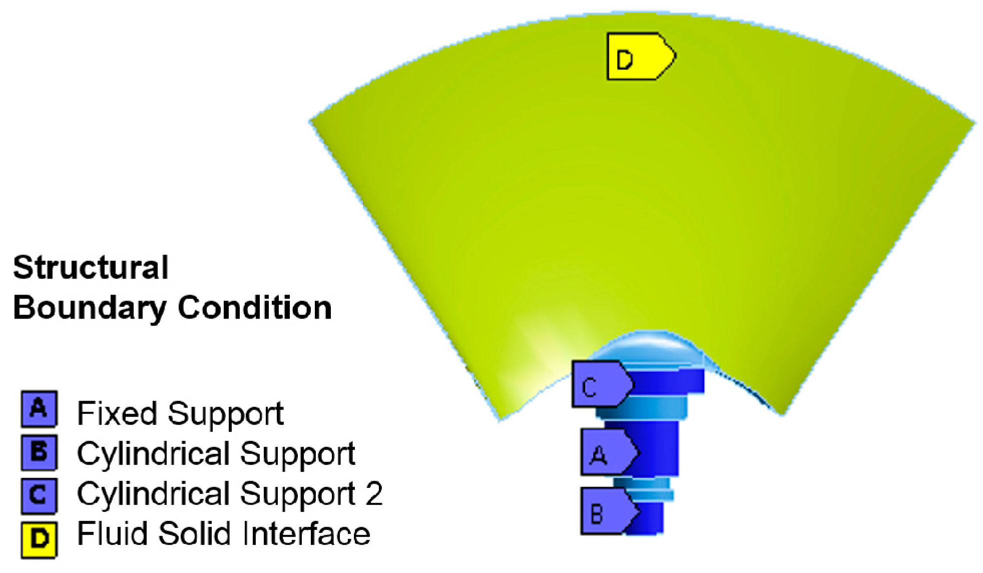
4.1. Structure Models and Boundary Conditions

Previously, a great deal of research has investigated an overall impeller as a research object and merely kept the profile of the objects for study, which did not involve discussion or analysis about their structural details. In this paper, the blade angle is adjusted by the manual adjustment of the worm and gear, and the inner structure of the impeller is complex, as demonstrated in Figure 5. Different blade structures determine different solution domains of finite element calculation. Therefore, the overall impeller should not be simply regarded as a solid structure during finite element calculation, meaning that a single blade of the impeller is selected as the object for structural calculation, which ensures more accurate simulation results.

The material of the impeller is ZG0Cr13Ni4CuMo with a density of 7730 kg/m³, a Young’s modulus of 203 GPa, Poisson’s ratio of 0.291, and yield strength of 550 MPa. As stress fields are concentrated on the roots of blades [3,4,30], the refinement of girds in this region is conducted. The sensibility analysis of grids is carried out by equivalent-stress finite element calculation of four schemes of impeller grids with different sizes (20 mm, 10 mm and two different refinements below 10 mm). It is found that results of two refinements below 10 mm were close, indicating a grid partition scheme of numerical convergence. A total of 126,136 units and 198,127 nodes are generated in the course of grid partition.

Boundary conditions of the impeller blade model involve structural constraints and loads [25,26,27,30,32,33]. Finite element calculation requires enough constraints to constrain the motion of the structure and prevent the rigid body displacement of the structure. Surface A is set as a fixed support, surface B and C are set as cylindrical supports, and surface D is set as the fluid–solid interface (Figure 6). Hence, a fixed constraint of cylindrical Surface A is conducted to constrain the motion of surface A in each direction. The cylinder constraint of cylindrical surfaces B and C is carried out to constrain the radial motion of blades. Blade surface D is defined as the interface of FSI to accomplish the information transferred between the flow fields and the solid fields. The time step and the total time obtained by finite element analysis are consistent with those of actual flow fields.

4.2. Computing Results and Analysis

To analyze the relationship between the dynamic stress characteristics and spatial positions of impeller blades under different working conditions, a static coordinate (x, y) and a rotating coordinate (ψ, ξ) are defined in Figure 7. In a rotating period, the position of an impeller blade is defined by the anti-clockwise rotation angle φ between the positive ψ axis of the rotating coordinate and positive y axis of the static coordinate. When the analyzed blade is located at the highest point of rotation and the blade’s axial direction points in the direction of gravity, that means φ = 0°.

Figure 8a shows the equivalent stress of the suction side of the impeller blade at φ = 0°, and a stress concentration region is found near the root and leading edge. This is consistent with the crack areas on the prototype blade, as shown in Figure 8b. This means the cracks may be influenced and caused by the high equivalent stress and stress concentration.

Figure 9 provides the changing rule of the maximum dynamic stress of blades within a spatial rotation cycle under different working conditions. Considering the influence of gravity, the maximum dynamic stress of the blade first increases and then decreases in an anticlockwise rotation cycle. The maximum equivalent stress appears at φ = 66° and is 150.25 MPa and 173.14 MPa under H = 2.5 m and H = 3 m working conditions, respectively. Under H = 3.5 m and H = 4 m working conditions, the maximum equivalent stress appears at φ = 140° and is 197.21 and 221.37 MPa, respectively; thus, the higher a head is, the greater its maximum dynamic stress would be. Meanwhile, the maximum dynamic stress of blades all appear on the suction surface near the leading edge of the blades and the root.

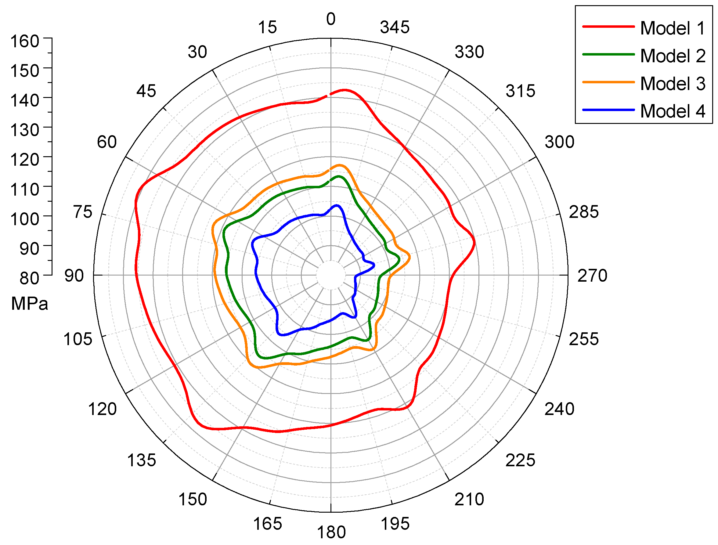
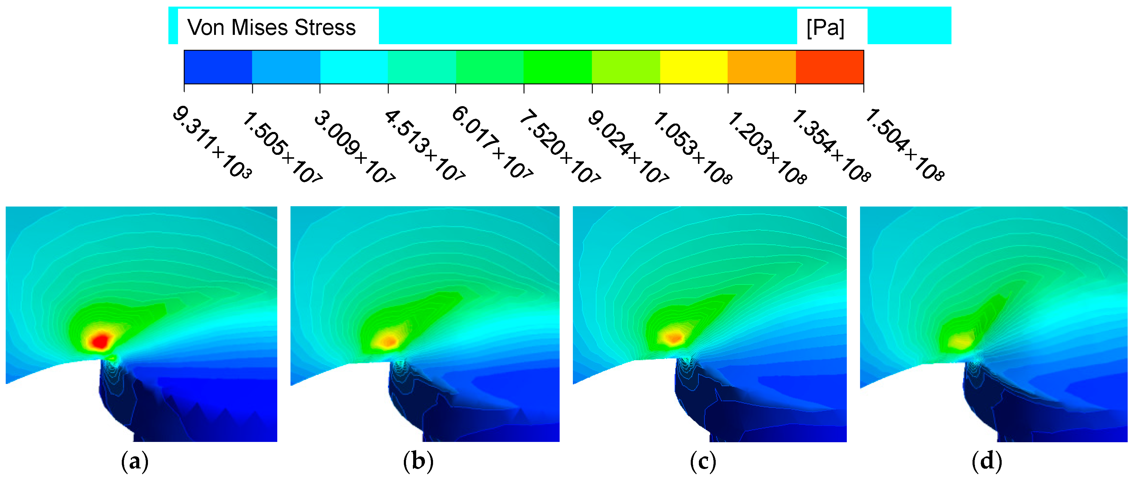
5. Stress State Improvement and Analysis

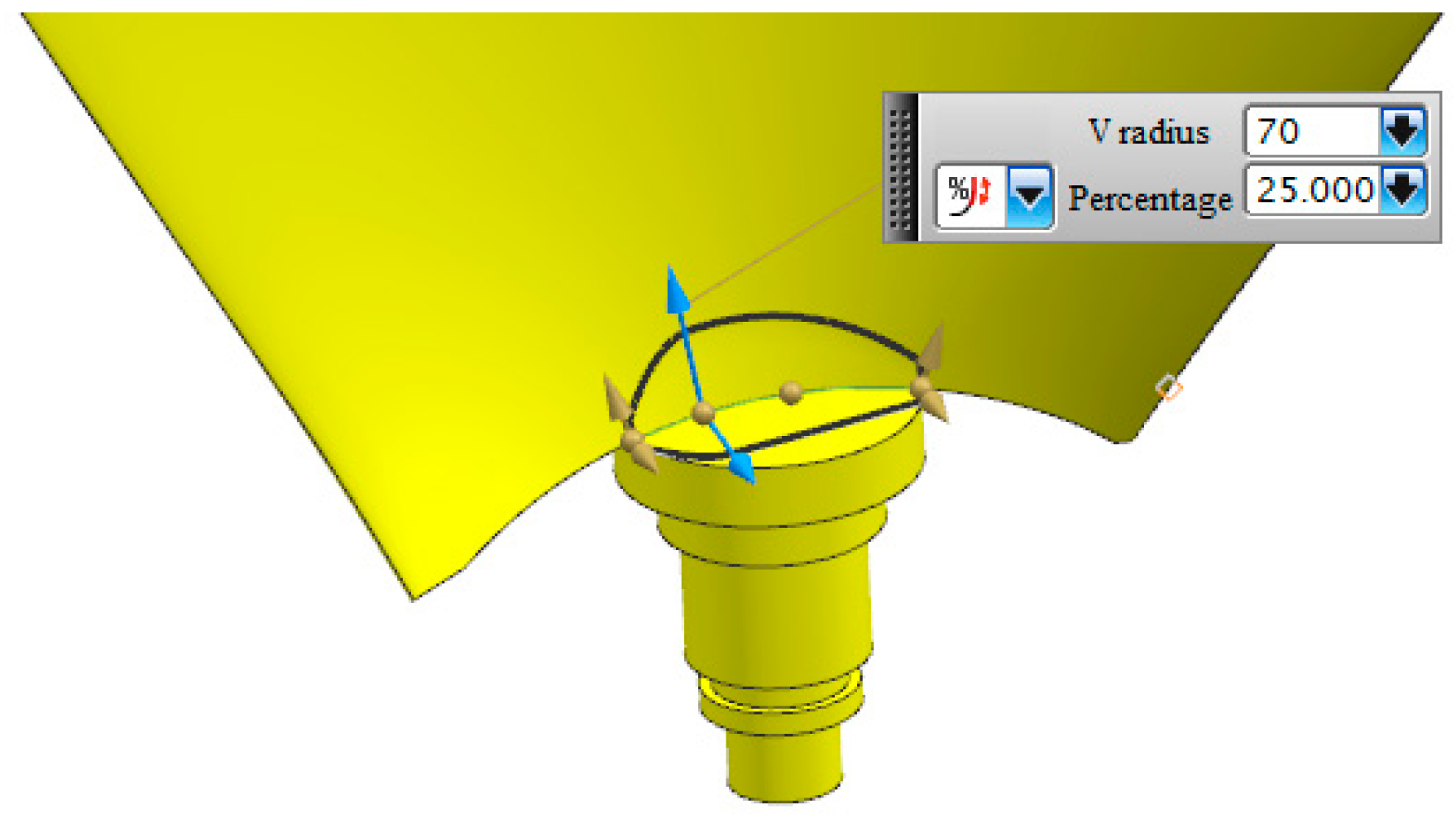
5.1. Improvement of Structural Models

In order to study the improving effects of maximum dynamic stress in the thickened blade root, four impeller blade models with different blade root thicknesses, namely models 1 to 4, are established as demonstrated in Figure 10. Figure 11 displays the design method for the modification of the blade root thicknesses, where the edges blend for the blade root with a V-shaped radius of 70 mm. The maximum radius of the edge blend appears where the percentage of the leading edge to the outlet edge is 25% (the stress concentration region of blade). As shown in Figure 11, the thicknesses of the blade roots and the percentages from the leading edge to the outlet edge of the four models are 50 mm and 50%, 50 mm and 25%, 70 mm and 50%, and 70 mm and 25%, respectively. It is important to note that all connections between the edge blends and the blades and shafts are smooth.

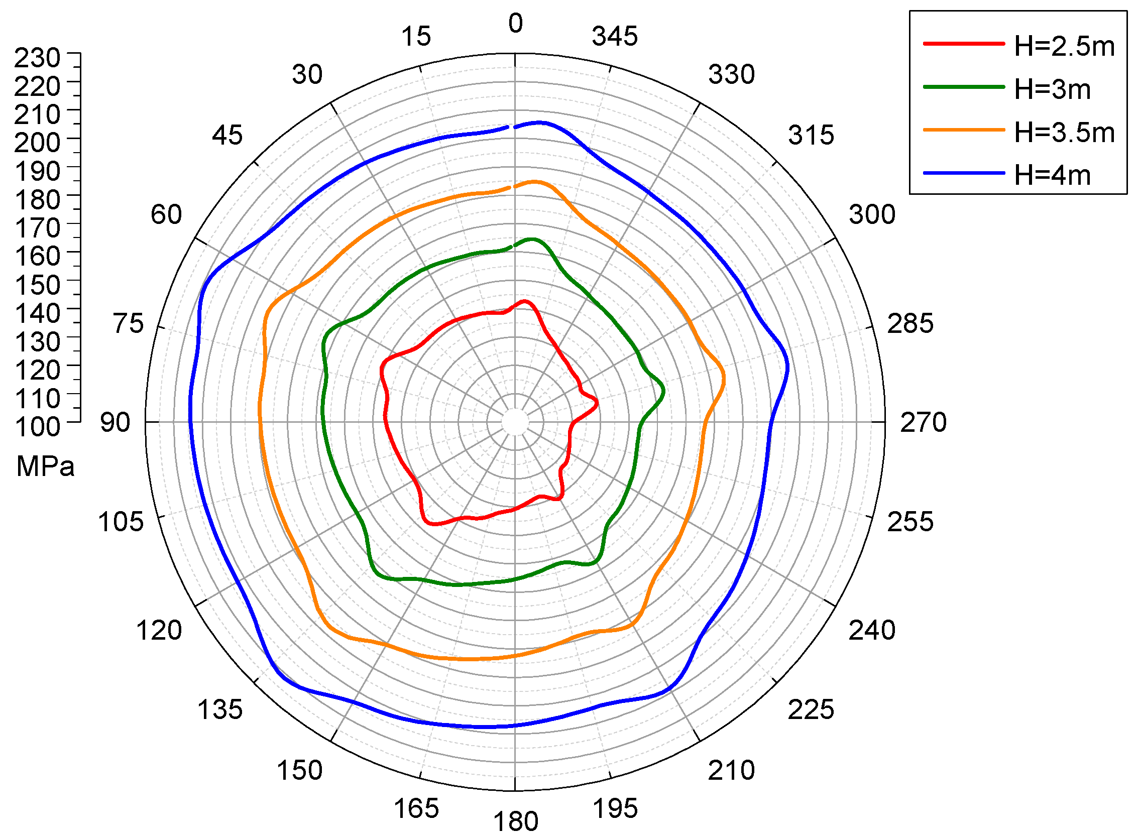
5.2. Analysis of Calculation Results

Through the FSI simulation of four blade models, the change rule of the maximum dynamic stress of four blade models over time within a cycle of spatial rotation in designed working conditions is figured out, as plotted in Figure 12. It is found that the maximum dynamic stress of the blade gradually reduces with the thickening of the blade root, and the maximum dynamic stress of Model 4 is only 108.41 MPa. Additionally, the local thickening effect on the stress-gathered area (Model 2) is slightly better than that for the whole root (Model 3).

Figure 13 presents the dynamic stress distribution near the leading edge of blades with different thicknesses of roots at φ = 66°. The stress concentration phenomenon of the blade is alleviated after the root thickening. In addition, the more the root thickens, the lower the stress concentration of the blades. However, the root thickening has no obvious influence on stress distribution beyond the stress concentration. Simultaneously, the fluid velocity and the torque generated by the work between the blade and fluid are smaller than those of other parts due to the blade root being close to the shaft; thus, the root thickening has little effect on the energy performance of the pump. In the design stage of axial-flow pump impeller blades, the thickening of the root, namely the asymmetric structure of stress concentration regions on the roots of leading edges, can be considered, which could effectively reduce the maximum dynamic stress of blades and improve the safety and stability of impeller blades.

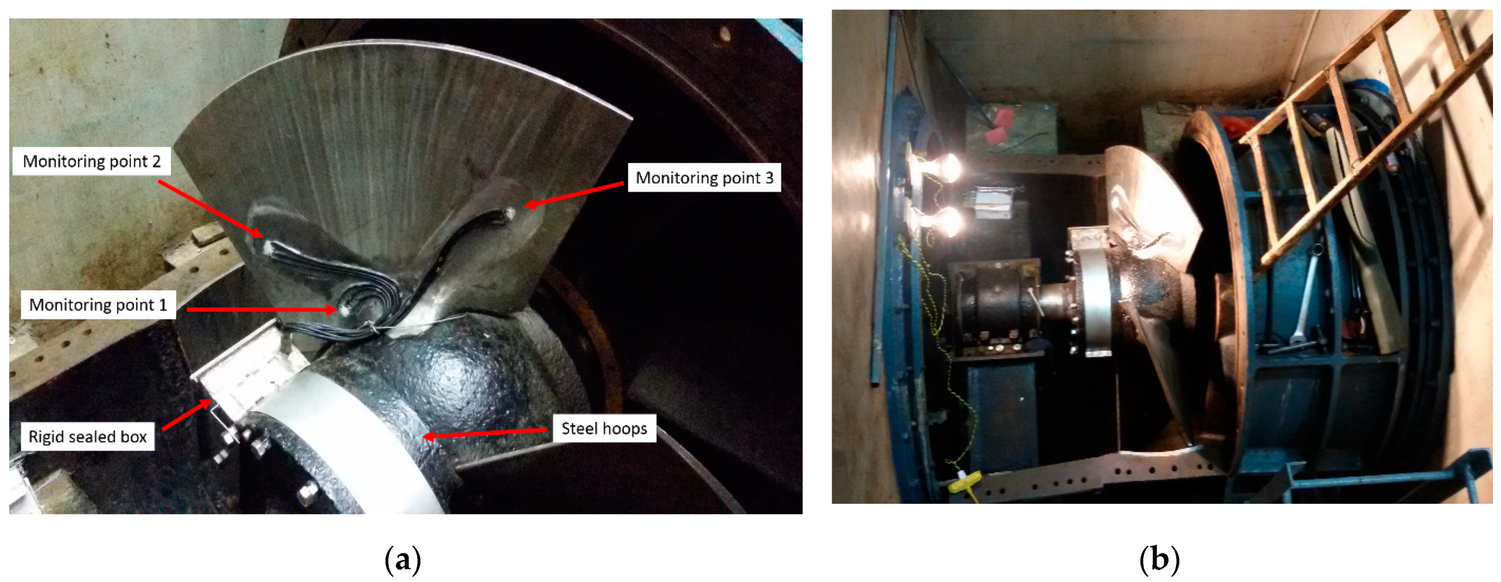
6. Design of Experimental Scheme and Result Analysis

6.1. Key Technological Solutions in the Stress Test of Impeller Blades

As the impeller blades of the pump rotate rapidly with high fluid pressure, several key technological problems need to be solved to test the working stress of blades under the special operating conditions: the protection of strain gauges and wires, the lead wires arrangement and seals, and the connection of the rotation signals to be measured and stationary instruments.

The protection of the strain gauges and wires under high water pressure, especially those on rotating components, are not only impacted by pressure load and temperature, but also by the inertia force and scouring force of water. Thus, strain gauges and wires without good protection may be separated from components, even leading to the failure of experiments. In this paper, we applied a coating to protect the strain gauges and wires. The coating method usually applies one or several layers of a chemical waterproof agent to the strain gauges and wires, which are characterized by good insulativity and bonding capacity, good plasticity, low elastic modulus, non-toxic and non-corrosive effects, stable pressure and temperature effects, solidification at room temperature, and convenience, etc.

High-strength insulated wires can be used as wires for strain measurement in high-pressure water. No damage of the wires is allowed, and strict waterproofing treatment of connections between the strain gauges and the wires, and the wires and splices, should be conducted.

In the experimental research, the most critical technical difficulty is the connection and transmission between stress test signals of impeller blades and test instruments in sealed and rotating conditions with pressure. In this condition, the conventional transmission modes, such as contact guyed, ring-brushing and mercury modes and non-contact induction and radio emission modes, cannot meet test requirements. As a result, a dynamic signal testing system characterized by a high accuracy, large capacity and offline collection and control is designed in this experiment, as shown in Figure 14. The standard deviation of the strain gauges is 2%, and the standard deviation of the wires is 0.5%. Therefore, the total standard deviation is 2.5%.

6.2. Experimental Comparison

As shown in Figure 15, the stress test of blades on prototypical pump units is carried out, and three strain rosettes are installed on the surface of the blade. The strain rosettes and wires are fixed and waterproof-sealed by the coating method. The test instruments are placed in a rigid sealed box fixed by a bolt hole and a steel hoop on the impeller.

After the installation and fixation of the on-site monitoring point and the experiment apparatus, the instrument is connected with a computer and made ready for tests after debugging and setting parameters relating to offline collection. After the cover and manholes are closed, the experiment preparation is completed. The water difference between the inlet reservoir and outlet reservoir is about 2.2 m.

To clarify the stress distribution of the structure, a strain gauge is attached, and the strain should be determined first so that the stress state of some points can be determined. If the direction of the principal stress is known, then the gauge should be attached along this direction, while if the direction of the principal stress is unknown, then the gauges should be attached along three different directions. On Point 1, three strain rosettes represented strain components at 0° (along the blade root and toward the radial direction of the blade), 45° (clockwise rotation of 45° along the blade root and toward the radial direction of the blade) and 90° (clockwise rotation of 90° along the blade root and toward the radial direction of the blade), respectively. The arrangement of the strain rosettes on Points 2 and 3 are similar to that for Point 1. After obtaining the strain components at each point, the dynamic stress states of each point can be determined through computational analysis.

6.3. Result and Error Analysis

The strain components in three directions are collected for each point. To eliminate vibrating disturbance beyond the unit, the dynamic strains are filtered and de-noised by filter function, and the new dynamic strains are acquired. After the computational analysis of the new dynamic strains, the dynamical stress states for each point are determined.

Table 2. Comparison between numerical results and experimental results for dynamic stress.

	Numerical Simulation		Experimental Value
	Maximum/MPa	Minimum/MPa	Maximum/MPa	Minimum/MPa
Point 1	151.0	119.4	123.9	94.6
Point 2	31.9	25.5	27.5	21.6
Point 3	14.4	10.4	11.8	7.9

lists the principal stresses on three monitoring points when their maximum strains appear within an average period of rotation.

Point 1 is located at the region where stress is concentrated and the maximum stress appears on the suction surface of the blade. The maximum dynamic stress at Point 1 is about 18% less than that in the simulation. The test results of both Points 2 and 3 are also less than their simulated values. The discrepancies between these two methods may be caused by the following reasons: the test heads are lower than the design heads, indicating that the water pressure load on the blade surface in the test is lower than that in the simulation; the specific location of the maximum dynamic stress changes within the stress concentration region and is not fixed, although Point 1 is designed to be located at the place with maximum dynamic stress, so it may be located on a point nearby during actual testing; and the installation of the offline data acquisition instrument on the hub and strain gauges and wires for stress tests may have certain influences on flow fields.

7. Conclusions

This paper has conducted a series of simulations of the unsteady flow of an axial-flow pump and the structure of a single impeller blade based on bidirectional FSI. In view of the gravity effect, the maximum dynamic stress of the blades shows a significant tendency of first increasing and then decreasing in an anticlockwise rotation cycle. The stress concentration occurred near the joint of the pressure and suction surface of the blade root and the shaft. The maximum dynamic stress of the blades appears at the joint area of the suction surface near the leading edge of the blade root and the shaft, which is a vulnerable region in terms of structural strength. The dynamic stress of the blades increases with the head improvement. The maximum equivalent stress is 221.37 MPa when the head reaches the peak value. The dynamic stress of blades is closely related to the water pressure load; therefore, the higher the head is during the operation of a pump, the greater the water pressure load on the blade surface will be. Based on the bidirectional FSI calculation of four blade models with different root thicknesses, the varying rule of the maximum dynamic stress and stress distribution of blades is analyzed. In Model 4, the maximum dynamic stress is only 108.41 MPa, which indicates that the stress concentration region with a properly thickened blade root could reduce the maximum stress and relieve the stress concentration of the blade effectively.

In terms of the stress measurement of high-speed rotating machinery under water, core issues in terms of sealing, data transfer and protection are discussed. By means of the designed stress testing system for a pump blade in the test, stress values on the surface of an impeller blade are collected effectively and are in good agreement with numerical simulation results. Therefore, according to the validated computing results, the FSI method could be adopted to evaluate the dynamic stress change rule of blades during the design stage of impellers, and stress distribution could be obviously improved by blade root thickening to enhance the security and stability of blades.

Future studies should also consider using measuring instruments of a smaller volume which could be equipped in the hub of the impeller to reduce the effect on the flow in the test. Furthermore, the dynamic stress under different impeller blade angles and the fatigue lifetime of the impeller blades would also be worthy of study.

References

1. Schneider, A.; Will, B.-C.; Bohle, M. Numerical evaluation of deformation and stress in impellers of multistage pumps by means of fluid structure interaction. In Proceedings of the ASME 2013 Fluids Engineering Division Summer Meeting, (FEDSM 2013), Incline Village, NV, USA, 7–11 July 2013. [Google Scholar]
2. Trivedi, C. A review on fluid structure interaction in hydraulic turbines: A focus on hydrodynamic damping. Eng. Fail. Anal. 2017, 77, 1–22. [Google Scholar] [CrossRef]
3. Kan, K.; Zheng, Y.; Zhang, X.; Yang, C.; Zhang, Y. Numerical study on unidirectional fluid-solid coupling of Francis turbine runner. Adv. Mech. Eng. 2015, 7. [Google Scholar] [CrossRef]
4. Pei, J.; Yuan, S.; Yuan, J. Dynamic stress analysis of sewage centrifugal pump impeller based on two-way coupling method. Chin. J. Mech. Eng. 2014, 27, 369–375. [Google Scholar] [CrossRef]
5. Campbell, R.; Paterson, E. Fluid–structure interaction analysis of flexible turbomachinery. J. Fluids Struct. 2011, 27, 1376–1391. [Google Scholar] [CrossRef]
6. Langthjem, M.A.; Olhoff, N. A numerical study of flow-induced noise in a two-dimensional centrifugal pump. Part I. Hydrodynamics. J. Fluids Struct. 2004, 19, 349–368. [Google Scholar] [CrossRef]
7. Angelidis, D.; Chawdhary, S.; Sotiropoulos, F. Unstructured Cartesian refinement with sharp interface immersed boundary method for 3D unsteady incompressible flows. J. Comput. Phys. 2016, 325, 272–300. [Google Scholar] [CrossRef] [Green Version]
8. Yang, X.; Sotiropoulos, F.; Conzemius, R.J.; Wachtler, J.N.; Strong, M.B. Large-eddy simulation of turbulent flow past wind turbines/farms: The Virtual Wind Simulator (VWiS). Wind Energy 2015, 18, 2025–2045. [Google Scholar] [CrossRef]
9. Posa, A.; Lippolis, A.; Verzicco, R.; Balaras, E. Large-eddy simulations in mixed-flow pumps using an immersed-boundary method. Comput. Fluids 2011, 47, 33–43. [Google Scholar] [CrossRef]
10. Favier, J.; Revell, A.; Pinelli, A. A Lattice Boltzmann–Immersed Boundary method to simulate the fluid interaction with moving and slender flexible objects. J. Comput. Phys. 2014, 261, 145–161. [Google Scholar] [CrossRef]
11. Sotiropoulos, F.; Yang, X. Immersed boundary methods for simulating fluid-structure interaction. Prog. Aerosp. Sci. 2014, 65, 1–21. [Google Scholar] [CrossRef]
12. Allison, T.C.; Lerche, A.H.; Moore, J.J. Experimental validation of empirical methods for dynamic stress prediction in turbomachinery blades. In Proceedings of the ASME 2011 Turbo Expo: Turbine Technical Conference and Exposition, (GT2011), Vancouver, BC, Canada, 6–10 June 2011; pp. 121–131. [Google Scholar]
13. Pei, J.; Yuan, S.; Yuan, J. Fluid-structure coupling effects on periodically transient flow of a single-blade sewage centrifugal pump. J. Mech. Sci. Technol. 2013, 27, 2015–2023. [Google Scholar] [CrossRef]
14. Benra, F.-K.; Dohmen, H.J.; Pei, J.; Schuster, S.; Wan, B. A Comparison of One-Way and Two-Way Coupling Methods for Numerical Analysis of Fluid-Structure Interactions. J. Appl. Math. 2011, 2011, 853560. [Google Scholar] [CrossRef]
15. Tang, X.; Wang, X.; Jia, Y. Strength analysis of bulb tubular pump impeller based on fluid-structure interaction. J. Drain. Irrig. Mach. Eng. 2014, 32, 921–926. [Google Scholar]
16. Lerche, A.H.; Moore, J.J.; White, N.M.; Hardin, J. Dynamic Stress Prediction in Centrifugal Compressor Blades Using Fluid Structure Interaction. In Proceedings of the ASME Turbo Expo 2012: Turbine Technical Conference and Exposition, Copenhagen, Denmark, 11–15 June 2012; pp. 191–200. [Google Scholar]
17. Li, W.; Ji, L.; Shi, W.; Zhou, L.; Jiang, X.; Zhang, Y. Vibration characteristics of the impeller at multi-conditions in mixed-flow pump under the action of fluid-structure interaction. J. Vibroeng. 2016, 18, 3213–3224. [Google Scholar] [CrossRef]
18. Hirsch, C. Numerical Computation of Internal and External Flows: The Fundamentals of Computational Fluid Dynamics; Elsevier: Amsterdam, The Netherlands, 2007. [Google Scholar]
19. Shi, L.; Tang, F.; Xie, R.; Zhang, W. Numerical and experimental investigation of tank-type axial-flow pump device. Adv. Mech. Eng. 2017, 9. [Google Scholar] [CrossRef] [Green Version]
20. Prasad, V. Numerical simulation for flow characteristics of axial flow hydraulic turbine runner. In Proceedings of the 2011 2nd International Conference on Advances in Energy Engineering, (ICAEE 2011), Bangkok, Thailand, 27–28 December 2011; pp. 2060–2065. [Google Scholar]
21. Alaimo, A.; Esposito, A.; Messineo, A.; Orlando, C.; Tumino, D. 3D CFD Analysis of a Vertical Axis Wind Turbine. Energies 2015, 8, 3013–3033. [Google Scholar] [CrossRef] [Green Version]
22. Zhou, D.; Chen, H.; Yang, C. A highly efficient Francis turbine designed for energy recovery in cooling towers. Adv. Mech. Eng. 2015, 7. [Google Scholar] [CrossRef] [Green Version]
23. Read, M.; Stosic, N.; Smith, I. Three-dimensional CFD Simulation of a Roots Blower for the Hydrogen Circulating Pump. In Proceedings of the International Compressor Engineering Conference 2018, West Lafayette, IN, USA, 9–12 July 2018. [Google Scholar]
24. Li, W.; Agarwal, R.K.; Ji, L.; Li, E.; Zhou, L. Numerical Simulation of Incipient Rotating Stall Characteristics in a Mixed-Flow Pump. In Proceedings of the AIAA Scitech 2019 Forum, San Diego, CA, USA, 7–11 January 2019; p. 2314. [Google Scholar]
25. Pei, J.; Dohmen, H.; Yuan, S.; Benra, F.-K. Investigation of unsteady flow-induced impeller oscillations of a single-blade pump under off-design conditions. J. Fluids Struct. 2012, 35, 89–104. [Google Scholar] [CrossRef]
26. Lomakin, V.O.; Banin, E.; Kuleshova, M.S.; Gouskov, A. Assessment of Hemolysis in a Ventricular Assist Axial Flow Blood Pump. Biomed. Eng. 2016, 50, 233–236. [Google Scholar]
27. Zhai, L.; Luo, Y.; Wang, Z.; Liu, X. 3D Two-way Coupled TEHD Analysis on the Lubricating Characteristics of Thrust Bearings in Pump-turbine Units by Combining CFD and FEA. Chin. J. Mech. Eng. 2016, 29, 112–123. [Google Scholar] [CrossRef]
28. Yousefi, H.; Noorollahi, Y.; Tahani, M.; Fahimi, R.; Saremian, S. Numerical simulation for obtaining optimal impeller’s blade parameters of a centrifugal pump for high-viscosity fluid pumping. Sustain. Energy Technol. Assess. 2019, 34, 16–26. [Google Scholar] [CrossRef]
29. Peng, G.; Wang, Z.; Yan, Z.; Liu, R. Strength analysis of a large centrifugal dredge pump case. Eng. Fail. Anal. 2009, 16, 321–328. [Google Scholar]
30. Saeed, R.; Galybin, A. Simplified model of the turbine runner blade. Eng. Fail. Anal. 2009, 16, 2473–2484. [Google Scholar] [CrossRef]
31. Yang, J.; Preidikman, S.; Balaras, E. A strongly coupled, embedded-boundary method for fluid–structure interactions of elastically mounted rigid bodies. J. Fluids Struct. 2008, 24, 167–182. [Google Scholar] [CrossRef]
32. Koloor, S.R.; Khosravani, M.R.; Hamzah, R.; Tamin, M. FE model-based construction and progressive damage processes of FRP composite laminates with different manufacturing processes. Int. J. Mech. Sci. 2018, 141, 223–235. [Google Scholar] [CrossRef]
33. Kan, K.; Zheng, Y.; Fu, S.; Liu, H.; Yang, C.; Zhang, X. Dynamic stress of impeller blade of shaft extension tubular pump device based on bidirectional fluid-structure interaction. J. Mech. Sci. Technol. 2017, 31, 1561–1568. [Google Scholar] [CrossRef]
Figure 1. Process of data exchange between fluid solver and structure solver.
Applsci 09 03601 g001
Figure 2. Geometric model of the whole flow system for the axial-flow pump.
Applsci 09 03601 g002
Figure 3. Grid of fluid calculation domain, (a) the whole calculation domain, (b) the main overflow components, (c) the root of the blade’s leading edge, and (d) the top of the blade’s leading edge.
Applsci 09 03601 g003aApplsci 09 03601 g003b
Figure 4. Comparison of numerical data and experimental data of hydraulic performances.
Applsci 09 03601 g004
Figure 5. Structure diagram of the impeller, (a) side view of middle section, (b) axial direction view of middle section, and (c) structural model of the blade.
Applsci 09 03601 g005
Figure 6. Boundary conditions of structure calculation.
Applsci 09 03601 g006
Figure 7. Definition of coordinate systems.
Applsci 09 03601 g007
Figure 8. Comparison of the simulated stress distribution of the impeller blade suction side at φ = 0° and cracks on the prototype impeller blade, (a) simulated region of stress concentration, (b) clustered cracks on the prototype impeller blade.
Applsci 09 03601 g008
Figure 9. Maximum dynamic stress change rules of blades under different heads.
Applsci 09 03601 g009
Figure 10. Finite element model of blades with four different root thicknesses: (a) Model 1, (b) Model 2, (c) Model 3, and (d) Model 4.
Applsci 09 03601 g010
Figure 11. Design method of blades with different root thicknesses.
Applsci 09 03601 g011
Figure 12. Maximum dynamic stress change rules of different root thickness blades.
Applsci 09 03601 g012
Figure 13. Maximum dynamic stress distribution of blades with different root thicknesses when φ = 66°: (a) Model 1, (b) Model 2, (c) Model 3, and (d) Model 4.
Applsci 09 03601 g013
Figure 14. A system of offline collection of dynamic signals.
Applsci 09 03601 g014
Figure 15. Monitoring the point arrangement and the on-site test instrument, (a) the arrangement of the on-site monitoring point, (b) the installation and fixation of a test instrument.
Applsci 09 03601 g015