Article

A Novel Hybrid Fuzzy Grey TOPSIS Method: Supplier Evaluation of a Collaborative Manufacturing Enterprise

1
State Key Laboratory of Fluid Power and Mechatronic Systems, Zhejiang University, Hangzhou 310027, China
2
School of Mechanical Engineering, Shandong University, Jinan 250061, China
3
Key Laboratory of High Efficiency and Clean Mechanical Manufacture (Ministry of Education), Shandong University, Jinan 250061, China
4
Department of Industrial Engineering and Management Systems, Amirkabir University of Technology, Hafez Ave. 424, Tehran 15875-4413, Iran
5
Department of Industrial Engineering, Tsinghua University, Beijing 100084, China
6
Institute of Systems Engineering, Macau University of Science and Technology, Macau 999078, China
*
Author to whom correspondence should be addressed.
Appl. Sci. 2019, 9(18), 3770; https://doi.org/10.3390/app9183770
Submission received: 11 July 2019 / Revised: 11 August 2019 / Accepted: 22 August 2019 / Published: 9 September 2019
(This article belongs to the Collection Advances in Automation and Robotics)

Abstract

:
Recently, there is of significant interest in developing multi-criteria decision making (MCDM) techniques with large applications for real-life problems. Making a reasonable and accurate decision on MCDM problems can help develop enterprises better. The existing MCDM methods, such as the grey comprehensive evaluation (GCE) method and the technique for order preference by similarity to an ideal solution (TOPSIS), have their one-sidedness and shortcomings. They neither consider the difference of shape and the distance of the evaluation sequence of alternatives simultaneously nor deal with the interaction that universally exists among criteria. Furthermore, some enterprises cannot consult the best professional expert, which leads to inappropriate decisions. These reasons motivate us to contribute a novel hybrid MCDM technique called the grey fuzzy TOPSIS (FGT). It applies fuzzy measures and fuzzy integral to express and integrate the interaction among criteria, respectively. Fuzzy numbers are employed to help the experts to make more reasonable and accurate evaluations. The GCE method and the TOPSIS are combined to improve their one-sidedness. A case study of supplier evaluation of a collaborative manufacturing enterprise verifies the effectiveness of the hybrid method. The evaluation result of different methods shows that the proposed approach overcomes the shortcomings of GCE and TOPSIS. The proposed hybrid decision-making model provides a more accurate and reliable method for evaluating the fuzzy system MCDM problems with interaction criteria.

1. Introduction

Multi-criteria decision making (MCDM) problems are utterly fatal and can be frequently observed academically in many domains, such as in manufacturing [1,2], finance [3], logistics [4], and the supply chain [5]. The rationality and correctness of the decision are quite crucial for a company. The development of an effective and efficient MCDM method to solve the optimization problems correctly is significant.
Conventionally, frequently-used MCDM methods include the goal programming method [6], the multi-attribute value theory [7], the multi-attribute utility method [8], the delaminating sequence method [9], the analytic hierarchy process (AHP) [10], the data envelopment analysis [11], the technique for order preference by similarity to ideal solution (TOPSIS) [12,13], grey comprehensive evaluation (GCE) method [14], fuzzy comprehensive evaluation [15], artificial neural networks [16] and some other fuzzy grey based hybrid MCDM approaches [17,18,19,20,21,22,23,24,25,26] Great progress has been made and compared with the earlier methods. However, there are still some shortcomings when dealing with the problems in real-life systems. It is universally acknowledged that the criteria are interactive [27,28,29] and for some qualitative criteria, we can only find the fuzzy evaluation rather than numerical values [30]. However, the hypothesis that the criteria are independent is diffusely used in these methods, and the evaluation values are aggregated through linear means, which usually leads to inadequate decisions.
The fuzzy integral is considered as an effective method to improve the limit since it can take into consideration the interactions among criteria expressed by fuzzy measures when aggregating the evaluation data [31,32,33,34]. The fuzzy integral is proposed by Sugeno [35] and further developed by many researchers. The fuzzy integral mainly includes the Sugeno fuzzy integral [36], the Choquet fuzzy integral [37], the (Y) fuzzy integral, the (N) fuzzy integral, the (H) fuzzy integral, the uncertain (H) fuzzy integral, the (T) fuzzy integral, the pseudo-additive and the Pan-integrals fuzzy integral [38]. Among these fuzzy integrals, the Choquet integral is the best for dealing with the nonlinear aggregation of MCDM problems since it can well express the interactions among criteria [39,40]. The fuzzy measures mainly include the nonadditive-measures, the quasi-additive-measures, the k-addictive fuzzy-measures, and the λ-fuzzy-measures [38,39]. Although the λ-fuzzy-measures can fully represent the interactions among criteria and are easy to calculate, they can only express one kind of interaction in one group of criteria. The k-addictive fuzzy-measure provides us a choice between the good expression ability and the simple computation, but we cannot obtain both simultaneously.
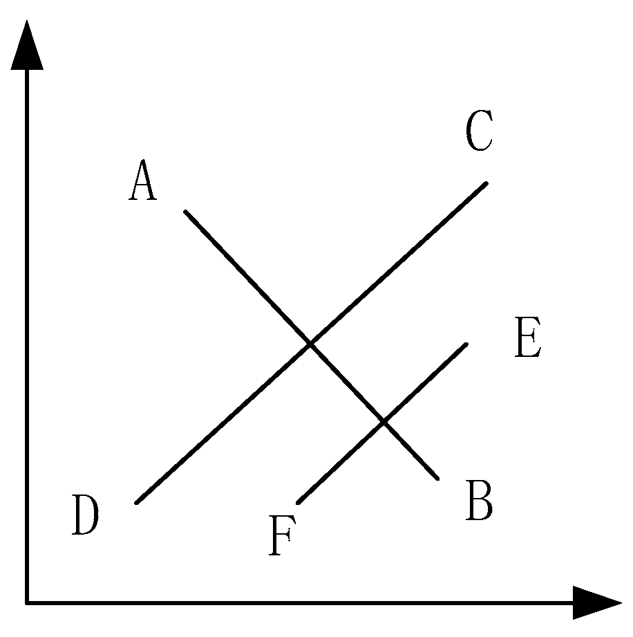
Among the conventional MCDM methods, the TOPSIS evaluates objects according to their difference in the comprehensive closeness degree. This evaluation is determined by the distance between the positive and negative ideal solution schemes [40]. It does not take into consideration the difference of shape of the scheme. The TOPSIS method fails under two conditions. In Figure 1, points A and B are positive and negative ideal solution schemes; Points C, D, E, and F are objects to evaluate. Generally, if the line AB is vertically divided by line CD, the distance between all the points on the straight line CD and point A are equal to that between these points and point B. The comprehensive close degrees of them are all 0.5. If line EF is vertically divided by line AB, the distance of points E and A is equal to that of points F and A. Furthermore, the distance of points E and B is equal to that of points F and B. The comprehensive close degrees of E and F are equal.
The GCE method depends on the grey correlation degree, which can reflect the closeness degree between the evaluation sequences of objects [41]. It does not take into account the number and distribution of samples and is easy to implement. However, most studies focus on the construction of the grey correlation coefficients. If the shapes of evaluation sequences of some objects are very similar, the GCE method may not be able to evaluate them properly. For example, assume that the evaluation sequences U1, U2, and U3 are shown in Figure 2. The correlation degree between U2 and U1 is the same as that between U3 and U1.
Other similar traditional methods, such as TOPSIS and GCE, assume that criteria are independent of each other. In this regard, to a great extent, it leads to limiting them when addressing some practical problems with interactive criteria. By considering these features of the TOPSIS and GCE approaches, this study develops a novel hybrid MCDM method called the fuzzy grey TOPSIS (FGT). By comparing the exiting methods, this research makes the following contributions.
First, the proposed method combines the GCE and TOPSIS, which improves the one-sidedness of the GCE and TOPSIS methods. Decision-makers can make a decision according to their preference through adjusting a parameter that reflects the weights of the shape and the distance factors.
Second, fuzzy measures and fuzzy integral are employed to express and integrate the interaction between the criteria that cannot be properly expressed through the existing methods.
Third, fuzzy numbers are used to help the experts make a more reasonable and accurate evaluation of some qualitative criteria.
The remainder of this paper is organized as follows: Section 2 is a literature review. Section 3 introduces the preliminaries. Section 4 presents the novel hybrid MCDM method that combines the fuzzy integral, the grey correlation, and TOPSIS. Section 5 utilizes an example of supplier evaluation of a collaborative manufacturing enterprise to illustrate the procedure, the feasibility, and effectiveness of the proposed method. Finally, conclusions are reached in Section 6.

2. Literature Review

Academically, many studies have been conducted on MCDM problems, and substantial progress has been made in this field. For example, Bouzarour-Amokrane et al. formulated a consensus bipolar method to solve the collaborative group MCDM problems considering the impact of human behavior, e.g., individualism, fear, caution [42]. The analysis results of the application example about real size wind farm implantation problem showed that this proposed method can be a useful decision-making tool to solve this problem [42]. Tchangani et al. proposed a bipolar aggregation method that combines weighted cardinal fuzzy measures, which can effectively overcome difficulties that dissuade the use of Choquet integral in practices to solve the fuzzy nominal classification in the MCDM problem [43]. Zhang et al. formulated a hybrid optimization approach combining the best worst method, grey relational analysis, and visekriterijumsko kompromisno rangiranje (VIKOR) to solve the MCDM problem in rail transit [44]. A multi-cell thin-walled aluminum energy-absorbing structure was applied to verify that this integrated method is valid and practical [44]. The results proved that this method provides an accurate and effective tool for the structural decision-making problem in rail transit [44]. Mousavi-Nasab and Sotoudeh-Anvari presented a new multi-criteria decision-making approach for the sustainable material selection problem [45]. Ten examples were applied to verify this proposed method [45].
TOPSIS and GCE are two of the several important methods in dealing with MCDM problems. Many researchers have a contribution to hybridization of MCDM techniques with some other method to make the best use of their advantages and bypass their disadvantages, as shown in Table 1 and Table 2. In addition, the fuzzy integral and fuzzy set are used to address the interaction among criteria which have been applied to many domains, as exposed in Table 3.

3. Preliminaries

3.1. The λ-Fuzzy-Measure and the Choquet Integral

In the FGT method, the weights of all subsets of a criterion set are expressed through the λ-fuzzy-measure.
Fuzzy-measures [39]: Assume that the criterion set X is nonempty and P(X) denotes its power set. If the set function g : P ( X ) [ 0 , 1 ] satisfies the following three axioms, then it is called a fuzzy-measure:
(1) Boundness
g ( ) = 0 , g ( X ) = 1 .
(2) Monotonicity
A ,   B P ( X ) ,   if   A B ,   then   g ( A ) g ( B ) .
(3) Weak continuity:
If   { A i } P ( X )   and   { A i }   is   monotonic ,   then     lim i = g ( A i ) = g ( lim i = A i ) .
λ-fuzzy-measures [39]: If the fuzzy-measure g satisfy the following axiom, then it is called λ-fuzzy-measures:
If   A , B P ( X )   and   A B = ,   then     λ [ 1 , ) ,   g ( A B ) = g ( A ) + g ( B ) + λ g ( A ) g ( B ) .
Let X = { x 1 , x 2 , , x n } be a finite set. If the fuzzy density of x i is g i , then g λ can be calculated as follows:
g λ ( { x 1 , x 2 , , x k } ) = i = 1 k g i + λ i 1 = 1 k 1 i 2 = i 1 + 1 k g i 1 g i 2 + + λ k 1 g 1 g 2 g k = 1 λ | i = 1 k ( 1 + λ g i ) 1 |
Choquet integral [79]: Without loss of generality, assume that the evaluation values on n criteria { f ( x i ) | i = 1 , 2 , , n } satisfy f ( x 1 ) f ( x i ) f ( x n ) . Then, the Choquet fuzzy integral of f ( x ) among g ( x ) on X is:
f d g = f ( x n ) g λ ( X n ) + [ f ( x n 1 ) f ( x n ) ] g λ ( X n 1 ) + + [ f ( x 1 ) f ( x 2 ) ] g λ ( X 1 )
where g λ ( X j ) = g λ ( { x 1 , x 2 , , x j } ) represents the fuzzy measure of the corresponding criterion set.

3.2. The Correlation Coefficients

Assume that the evaluation matrix is
C m × n = [ C 1 ( 1 ) C 1 ( 2 ) C 2 ( 1 ) C 2 ( 1 ) C 1 ( n ) C 2 ( n ) C m ( 1 ) C m ( 2 ) C m ( n ) ] ,
where the i-th row represents the evaluation sequence of the i-th object. {C*(.)} = {C*(1), C*(2),…,C*(n)} is selected as the reference sequence where C * ( l ) represents the best of the l-th criterion. The correlation coefficient vector of the i-th alternative sequence related to the reference sequence is denoted as ξ i * = {   ξ i * ( 1 ) ,   ξ i * ( 2 ) , ,   ξ i * ( n ) } . We then have [80]:
ξ i * ( k ) = min i min k | C * ( k ) C i ( k ) | + ρ max i max k | C * ( k ) C i ( k ) | | C * ( k ) C i ( k ) | +   ρ max i max k | C * ( k ) C i ( k ) |
where the resolution ratio ρ [ 0 , 1 ] is usually assigned as 0.5.
The absolute correlation degree can be found by
r i = j = 1 n ( w j × ξ i * ( j ) ) .
The bigger the degree value is, the better the object is.

3.3. The Triangle Fuzzy Number

Triangle fuzzy number [81]: The membership function of the fuzzy number n ˜ = ( n 1 , n 2 , n 3 ) is defined as
f ( x ) = { x n 1 n 2 n 1 , n 1 x < n 2 x n 3 n 2 n 3 , n 2 x n 3 0 , other ,
where   0 n 1 n 2 n 3 .
Let m ˜ = ( m 1 , m 2 , m 3 )   and   n ˜ = ( n 1 , n 2 , n 3 ) be fuzzy numbers. Then,
m ˜ n ˜ ( m 1 + n 1 , m 2 + n 2 , m 3 + n 3 ) .

3.4. The Entropy Weight Method

With the premise that there are m objects and n criteria for evaluation, which form the evaluation matrix Z = { z i j ; i = 1 ,   2 , , m ; j = 1 ,   2 , , n } , the weights of all criteria can be calculated through the entropy weight method [82], as shown in Equation (7).
{ ω j = 1 H j i = 1 n ( 1 H j ) H j = i = 1 m P i j ln ( P i j ) ln ( m ) P i j = z i j i = 1 m z i j .

4. The Fuzzy Grey TOPSIS Method

4.1. Background

Assume that there are m objects to be evaluated. The objects set is A = { a 1 , a 2 , , a m } . There are p experts involved in the evaluation and decision. The experts set is denoted as E = { E 1 , E 2 , , E p } .
To evaluate these objects, the experts should construct a reasonable and effective criterion system according to the feature of the considered problem and the purpose and preference of the decision-maker. As it is widely acknowledged, a real-life system usually contains some unknown information, i.e., it is a grey system. Therefore, some qualitative criteria need to be employed to evaluate the system. In addition, we also need a few quantitative criteria for some measurable aspects.
Assume that among n criteria, some qualitative and some quantitative criteria are considered. The criterion set is X = { x 1 , x 2 , , x n } . For the convenience of expression, assume that x 1 ,   x 2 , ,   x i are quantitative criteria and x i + 1 , ,   x n are qualitative.

4.2. The Procedure of Fuzzy Grey TOPSIS

Step 1: Find the evaluation data.
Step1.1: Obtain evaluation data of qualitative criteria.

4.2.1. Obtain the Fuzzy Linguistic Value and Transform it into Fuzzy Numbers

To make the experts’ evaluation more accurate, a set of fuzzy linguistic values is set up and noted as { Superb ,   Good ,   Normal ,   Bad ,   Terrible } ( { S ,   G ,   N ,   B ,   T } for short). The evaluation data of qualitative criteria are given by experts in the form of fuzzy linguistic values that correspond to fuzzy numbers. Mapping rules are shown in Table 4.
The linguistic variable evaluation matrixes are transformed as fuzzy number matrixes, as shown below.
J ˜ 1 = [ j ˜ 1 ( n i + 1 ) 1 j ˜ 1 n 1 j ˜ 1 ( n i + 1 ) k j ˜ 1 n k ] J ˜ m = [ j ˜ m ( n i + 1 ) 1 j ˜ m n 1 j ˜ m ( n i + 1 ) k j ˜ m n k ] ,
where J ˜ i represents the fuzzy number matrix of the i-th object j ˜ i j k represents the fuzzy number corresponding to the k-th expert’s evaluation of the i-th object on the j-th criterion.
The fuzzy number evaluation values of k experts need to be integrated into one fuzzy number according to Equation (6). The fuzzy evaluation matrix J ˜ can be given as
J ˜ = [ j ˜ 1 ( n - i + 1 ) j ˜ 1 n j ˜ m ( n - i + 1 ) j ˜ m n ] ,
where j ˜ i j represents the fuzzy number of the i-th object on the j-th criterion.

4.2.2. Defuzzify the Fuzzy Numbers

The fuzzy numbers need to be defuzzified into numerical values to take part in the calculation procedure later. There are many defuzzification methods, each of which has its advantages and limits. Three methods are adopted in this paper. In the case that the operation is too simple, and its effectiveness cannot be verified [83], the mean value of the results of the three methods is taken. Fuzzy numbers j ˜ i k = ( a i k , b i k , c i k ) can be defuzzicated through the three methods stated as follows:
(1) Distance measure method [81]:
M i k 1 = d i k d i k + d i k * .
If the optimal fuzzy evaluation value is defined as j ˜ i k * = ( 1 , 1 , 1 ) and the worst fuzzy evaluation value is defined as j ˜ i k = ( 0 , 0 , 0 ) , then
d i k = 1 4 ( a i k 2 + 2 b i k 2 + c i k 2 ) ,
d i k * = 1 4 [ ( 1 a i k ) 2 + 2 ( 1 b i k ) 2 + ( 1 c i k ) 2 ] .
(2) Central value method [84]:
M i k 2 = b i k + ( c i k b i k ) ( b i k a i k ) 6 = 4 b i k + c i k + a i k 6
(3) Gravity method [84]:
M i k 3 = { a i k ,   a i k = b i k = c i k ( c i k ) 2 ( a i k ) 2 + b i k ( c i k a i k ) 3 ( c i k a i k ) ,   o t h e r w i s e .
The numerical value j i k can be found by taking the mean value of the three results, i.e.,
j i k = M i k 1 + M i k 2 + M i k 3 3 .
The fuzzy evaluation matrix J ˜ can be transformed into a numerical evaluation matrix J * .
J * = [ j 1 ( n i + 1 ) j 1 n j m ( n i + 1 ) j m n ] .
Step1.2: Find evaluation data of quantitative criteria.
The evaluation data of a few numerical criteria { j k 1 , j k 2 , , j k i | k = 1 , 2 , , m } are obtained through statistics and measurement methods. By seaming the numerical evaluation matrix of qualitative and quantitative criteria, the evaluation matrix J can be found, as shown below,
J = [ j 11 j 1 n j m 1 j m n ] ,
where J k l represents the evaluation value of the k-th object on the l-th criterion, k = 1 ,   2 ,   ,   m ,   l = 1 ,   2 ,   ,   n .
Step 2: Standardize evaluation matrix.
To eliminate the influence of dimension and order of magnitude, the evaluation matrix J needs to be standardized according to Equation (14):
c i k = j i k j k ¯ S k ,
where j ¯ k is the mean and S k is the standard deviation of the evaluation values of the k-th criterion.
In that way, the standardized evaluation matrix C can be found.
C = [ c 11 c 1 n c m 1 c m n ] ,
where J k l represents the standardized evaluation value of the k-th object on the l-th criterion, k = 1 ,   2 ,   ,   m ,   l = 1 ,   2 ,   ,   n .
Theorem 1.
The standardization transformation satisfies the following two axioms:
(1) Isotonicity:
If   j x k < j y k ,   then   c x k < c y k .   If   j x k > j y k ,   then     c x k > c y k .
Proof. 
If j x k < j y k , then j x k j k ¯ < j y k j k ¯ . Thus j x k j k ¯ S k < j y k j k ¯ S k , namely, c x k < c y k . Similarly, if j x k > j y k , then c x k > c y k .
(2) Difference remaining:
  x , y , p , q ,   j x k   j y k j p k   j q k = c x k   c y k c p k   c q k .
 □
Proof. 
  x , y , p , q ,   c x k   c y k c p k   c q k
= ( j x k j k ¯ S k j y k j k ¯ S k ) / ( j p k j k ¯ S k j q k j k ¯ S k ) = j x k   j y k j p k   j q k .
 □
Step 3: Obtain weights of criteria.
To aggregate the evaluation data, some series of weights that are reasonable and accurate as much as possible is certainly needed. The weights are considered in two aspects. On the one hand, the objective weights are calculated through the entropy weight method such that the influence of data can be considered. On the other hand, the subjective weights are given by the experts to express the decision preference. Finally, the weighted average value of objective and subjective weights is taken.
Step 3.1: Calculate objective weights of criteria.
The objective initial weights are mainly calculated through the entropy weight method. However, some minor amendments are made to make the formula meaningful. By using the data of standardized evaluation matrix C = { c i j , i = 1 ,   2 , , m , j = 1 ,   2 , , n } , the objective weights vector ω 1 = [ ω 1 1 , ω 2 1 , , ω n 1 ] can be calculated according to Equation (15).
{ ω j 1 = 1 H j j = 1 n ( 1 H j ) H j = i = 1 m ( 1 + P i j ) ln ( 1 + P i j ) ln ( m ) P i j = c i j i = 1 m | c i j | .
Step 3.2: Obtain subjective weights of criteria.
The subjective weights vector ω 2 = [ ω 1 2 , ω 2 2 , , ω n 2 ] is given by experts.
Step 3.3: Integrate objective and subjective weights.
The comprehensive weights vector ω 0 = [ ω 1 0 , ω 2 0 , , ω n 0 ] can be found according to Equation (16).
ω j 0 = θ ω j 1 + ( 1 θ ) ω j 2 ,
where the parameter θ ( 0 , 1 ) is determined by the decision maker according to the degree of trust in objective data and subjective judgment of experts. We set it as 0.5 in this paper.
Step 4: Identification of λ-fuzzy-measures.
It is generally believed that many interactions exist among criteria. If we integrate the evaluation matrix by weights only, the interactions are ignored, which will lead to an inadequate decision. Thus, the λ-fuzzy-measures are employed here to express the interactions.
Let us regard the comprehensive weights vector ω 0 = [ ω 1 0 , ω 2 0 , , ω n 0 ] as the fuzzy densities. The parameter λ can be obtained by Equation (17):
1 λ | i = 1 n ( 1 + λ ω i 0 ) 1 | = 1 .
Note that the comprehensive weights vector ω 0 = [ ω 1 0 , ω 2 0 , , ω n 0 ] and the parameter λ are obtained. All the fuzzy-measures { ω Q ; Q P ( X ) } can be calculated according to Equation (18), where P ( X ) is the power set of X .
ω Q = i = 1 p ω i 0 + λ i 1 = 1 p 1 i 2 = i 1 + 1 p ω i 1 0 ω i 2 0 + + λ p 1 ω 1 0 ω 2 0 ω p 0
Step 5: Calculate the grey fuzzy correlation degree.
Step 5.1: Calculate correlation coefficients.
To describe the difference in shapes of all objects, their positive and the negative correlation coefficients need to be calculated. First of all, the positive and the negative ideal solution schemes C + = [ c 1 + , c 2 + , , c n + ] and C = [ c 1 , c 2 , , c n ] should be selected. With the premise that J + represents the set of some criteria which are the bigger the better, and J represents the set of some criteria which are the smaller the better, the vector C + and C can be determined according to Equations (19) and (20).
c j + = { max 1 i m ( c i j ) , if j J + min 1 i m ( c i j ) , if j J ,
c j - = { min 1 i m ( c i j ) , if j J + max 1 i m ( c i j ) , if j J .
The positive correlation coefficients { ξ i j + , i = 1 , 2 , , m , j = 1 , 2 , , n } and the negative correlation coefficients { ξ i j , i = 1 , 2 , , m , j = 1 , 2 , , n } of the j-th criterion can be calculated according to Equations (21) and (22):
ξ i j + =   min i min k | c i j + c i j | + ρ max i max k | c i j + c i j | | c i j + c i j | +   ρ max i max k | c i j + c i j | ,
ξ i j =   min i min k | c i j c i j | + ρ max i max k | c i j c i j | | c i j c i j | +   ρ max i max k | c i j c i j | .
Then the positive correlation matrix ξ + and the negative correlation matrix ξ can be obtained as
ξ + = [ ξ 11 + ξ 1 n + ξ m 1 + ξ m n + ] ,
ξ = [ ξ 11 ξ 1 n ξ m 1 ξ m n ] .
Step 5.2: Calculate the grey fuzzy Choquet integral.
To take the interactions among criteria into account, the Choquet fuzzy integral is used to integrate the correlation coefficients of every object. The positive grey fuzzy integral vector R + = [ R 1 + , R 2 + , , R m + ] and the negative grey fuzzy integral vector R = [ R 1 , R 2 , , R m ] can be calculated as follows.
Definition 1.
(Positive grey fuzzy Choquet integral): Let correlation coefficients { ξ i j + ; i = 1 , 2 , , m , j = 1 , 2 , , n } be reordered in an ascending order such that ξ i 1 + ξ i j + ξ i n + . The positive grey fuzzy Choquet integral of the i-th object is defined as
R i + = ξ i n + ω 12 n + [ ξ i n 1 + ξ i n + ] ω 12 ( n 1 ) + + [ ξ i 1 + ξ i 2 + ] ω 1 ,
where ω 12 k represents the weight of the set { x 1 , x 2 , , x k } ( k n ) after rearrangement.
Definition 2.
(Negative grey fuzzy Choquet integral): Let correlation coefficients { ξ i j ; i = 1 , 2 , , m , j = 1 , 2 , , n } be reordered in an ascending order such that ξ i 1 ξ i j ξ i n . The negative grey fuzzy Choquet integral of the i-th object is defined as
R i = ξ i n ω 12 n + [ ξ i n 1 ξ i n ] ω 12 ( n 1 ) + + [ ξ i 1 ξ i 2 ] ω 1 .
Step 6: Calculate fuzzy distance to ideal solution.
To embody the difference the in distance of all objects, the distance between all objects to the positive and negative ideal solution schemes should be obtained. The Choquet fuzzy integral should also be employed to amend the Euclidean distance such that the interactions can be expressed in the distance.
Definition 3.
(Positive fuzzy ideal solution distance): Let positive distances of all criteria { d i j + = ( c i j c j + ) 2 ; i = 1 , 2 , , m , j = 1 , 2 , , n } be reordered in an ascending order such that d i 1 + d i j + d i n + . The positive fuzzy ideal solution distance of the i-th object is defined as
D i + = [ d i n + ω 12 n + ( d i n 1 + d i n + ) ω 12 ( n 1 ) + + ( d i 1 + d i 2 + ) ω 1 ] 1 2 .
Definition 4.
(Negative fuzzy ideal solution distance): Let negative distances of all criteria { d i j = ( c i j c j ) 2 ; i = 1 , 2 , , m , j = 1 , 2 , , n } be reordered in an ascending order such that d i 1 d i j d i n . The positive ideal solution fuzzy distance of the i-th object is defined as
D i = [ d i n ω 12 n + ( d i n 1 d i n ) ω 12 ( n 1 ) + + ( d i 1 d i 2 ) ω 1 ] 1 2 .
Step 7: Get grey fuzzy TOPSIS.
The positive grey fuzzy Choquet integral and the negative ideal solution distance depend on the close degree to the positive ideal solution of each scheme on the shape and distance, respectively. Their combination can represent the comprehensive close degree to the positive ideal solution of each scheme. Analogously, the combination of negative grey fuzzy Choquet integral and the positive ideal solution distance can characterize the close degree to the negative ideal solution of each scheme. To express the effects of R + , R , D + ,   and   D , they need to be normalized before combination.
N i n e w = N i max 1 i m N i ; i = 1 , 2 , , m ,
where N i represent R + ( R ; D + ; D ) , respectively.
For the conciseness, the normalized values of them are still denoted as R + , R , D + , D , respectively. The positive comprehensive proximity degree vector S + = [ S 1 + , S 2 + , , S m + ] and the negative comprehensive proximity degree vector S = [ S 1 , S 2 , , S m ] can be obtained by combining R + , R , D + ,   and   D with a proper weight parameter p according to Equation (28).
{ S i + = p R i + + ( 1 p ) D i ; i = 1 , 2 , , m S i = p R i + ( 1 p ) D i + ; i = 1 , 2 , , m ,
where parameter p ( 0 , 1 ) is determined by the decision-maker’s preference.
The comprehensive evaluation vector C S = [ C S 1 , C S 2 , , C S m ] can be calculated by Equation (29).
C S i = S i + S i - + S i + ; i = 1 , 2 , , m .
The m objects can be evaluated reasonably according to the comprehensive evaluation vector C S = [ C S 1 , C S 2 , , C S m ] . The object whose comprehensive evaluation value is big is better than the one whose comprehensive evaluation value is small.
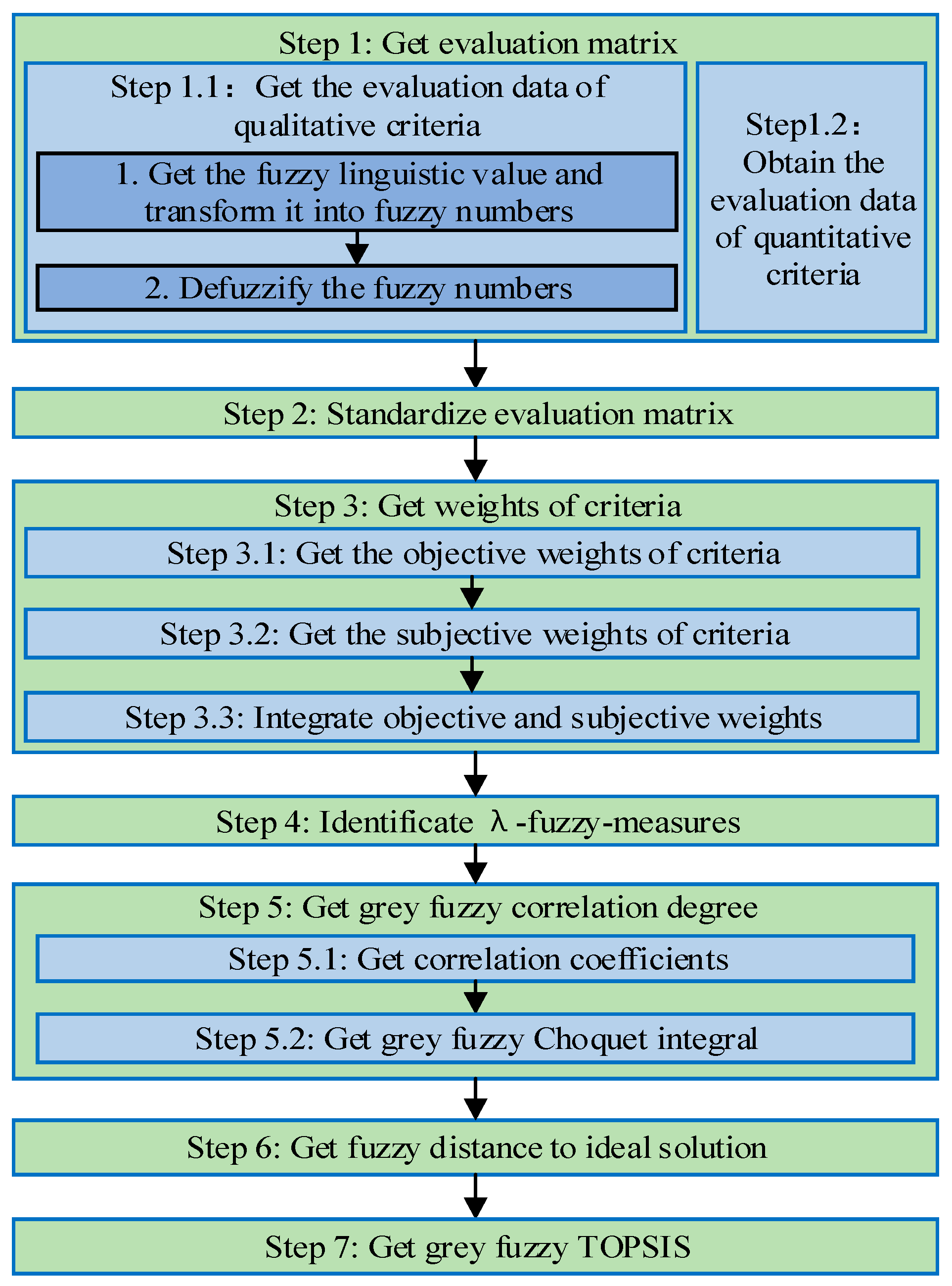
The flow chart of the proposed method is given in Figure 3.

5. An Illustrative Example

To verify the feasibility and effectiveness of the proposed method, an illustrative example of supplier evaluation of a collaborative manufacturing enterprise is given in this paper. The result was compared with GCE and TOPSIS. This example has six alternatives A = { A 1 ,   A 2 ,   A 3 ,   A 4 ,   A 5 ,   A 6 } and 12 experts E = { E 1 ,   E 2 , ,   E 12 } .
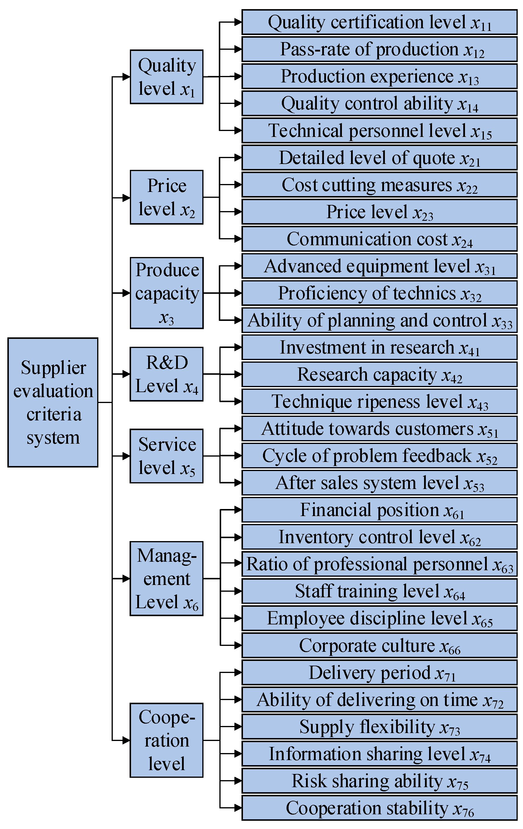
According to the feature of the supplier evaluation of the collaborative manufacturing enterprise and the purpose and preference of the decision-maker, a reasonable and effective criterion system was constructed by experts, as shown in Figure 4.

5.1. Conducting the Proposed Method

The detailed process of the proposed method to solve this example is illustrated below. Each level is addressed one by one. We illustrate the quality level in detail only for economy of space.
Step 1: Get the evaluation matrix.
The fuzzy linguistic value evaluation matrices { j ˜ 1 ,   j ˜ 2 ,   j ˜ 3 ,   j ˜ 4 ,   j ˜ 5 ,   j ˜ 6 } are shown as follows, in which the mapping rules of linguistic variables and fuzzy number are given in Table 4.
J ˜ 1 = [ S S G S S G S S S G S S 0.98 G N G G N N G G G S G G S G S S S S N G G S G S G G S G G S G S S G S S ] ,
J ˜ 2 = [ B B B T T B B B B T B B 0.83 N N N G N N N G N N G G N G G N G S G G G G N G G G G S G G G G S G N G ] ,
J ˜ 3 = [ S S G S S S G G S G S S 0.92 N N N G N N N G N B N N N N N B N B B B N N N B N N N B N N N G G N N N ] ,
J ˜ 4 = [ G G G G G G S G G G N G 0.93 G G G N G G G G S G G S G G G N N G G G G S G G G N N G G G G G N G G G ] ,
J ˜ 5 = [ G S S S S S S G S S S S 0.99 N N G G N N N G N G N N N G N G N N N N N G N N N N G N N N G N N N N N ] ,
J ˜ 6 = [ S S G G S S S S S G S S 0.95 G G G N G G N N G G G G N N N N G G N N G N N G N N N G N N N G N N N G ] ,
where each matrix represents the evaluation data of an alternative, and each row in the matrix represents the evaluation data of one qualitative criterion given by 12 experts expect for the second row of each matrix that is the evaluation data of the quantitative criterion and has just one value. In fact, we can give the evaluation of qualitative criteria and quantitative criteria, respectively, but for the convenience of writing, we give them in one matrix.
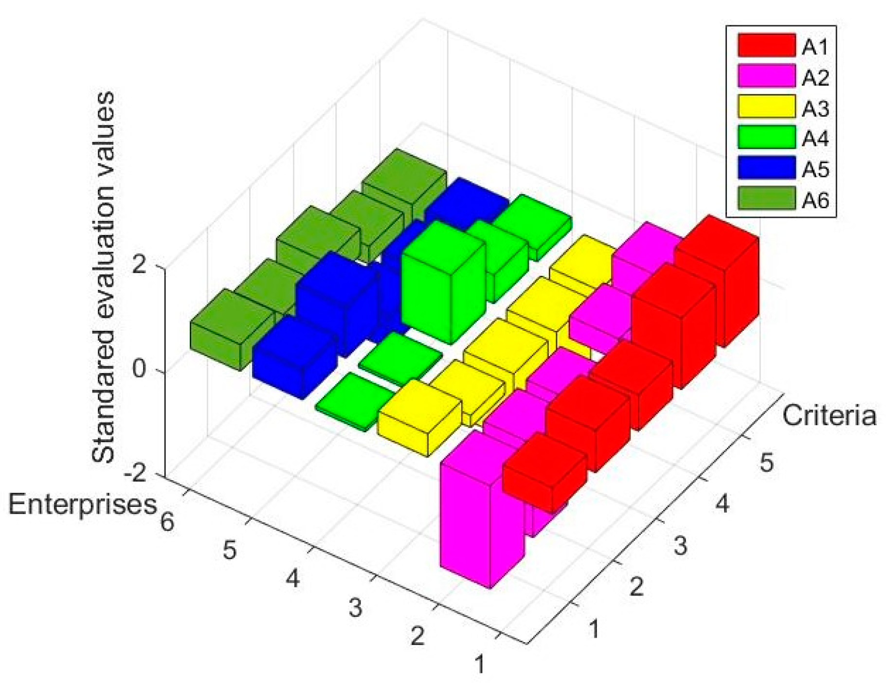
We transformed the fuzzy linguistic values into fuzzy numbers according to (6). Then these fuzzy numbers were aggregated according to Equation (6) and defuzzified according to Equations (8)–(13). Then the evaluation matrix J was found as follows:
J = [ 0.8295 0.9800 0.6635 0.7839 0.7858 0.2579 0.8300 0.5662 0.6635 0.7111 0.8150 0.9200 0.5166 0.4172 0.5166 0.6965 0.9300 0.7111 0.6800 0.6489 0.8440 0.9900 0.5662 0.5497 0.5331 0.8295 0.9500 0.6489 0.5662 0.5497 ] ,
where each row represents the evaluation data of an alternative, and each column represents the evaluation data of a criterion.
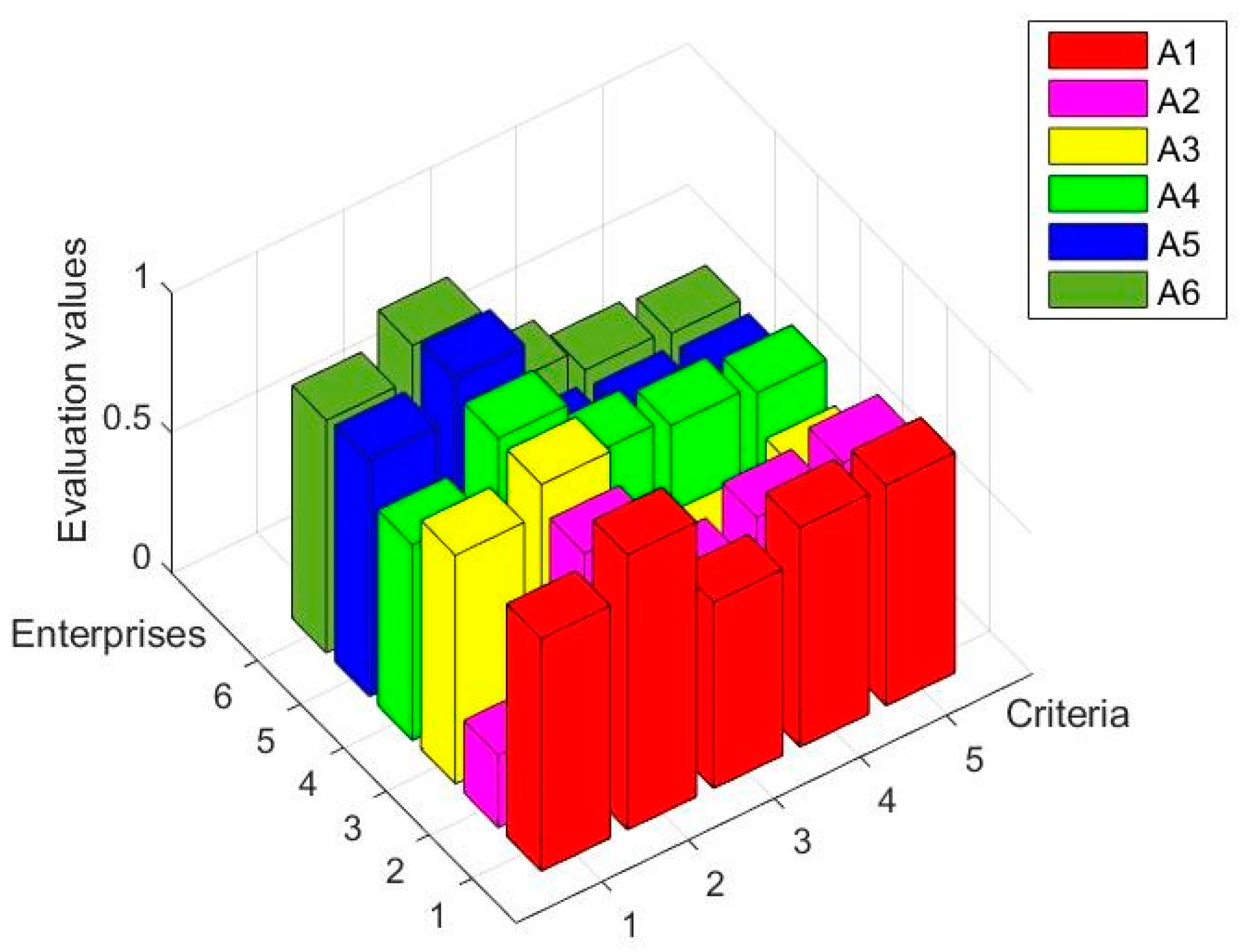
The 3-dimensional histogram of J is portrayed in Figure 5.
Step 2: Standardize evaluation matrix.
The evaluation matrix J can be standardized as C according to Equation (14), as shown as below.
C = [ 0.5129 0.8115 0.6977 1.3681 1.4790 1.9837 1.7970 0.6225 0.4202 0.7949 0.4494 0.2319 1.2968 1.5178 0.9849 0.0679 0.0580 1.3439 0.5502 0.2263 0.5763 0.9854 0.6225 0.4755 0.8334 0.5129 0.2898 0.5002 0.3452 0.6819 ] .
The 3-dimensional histograms of C is depicted in Figure 6.
Step 3: Obtain weights of criteria.
Step 3.1: Calculated the objective weights of criteria.
The objective weight vector which was calculated by Equation (15) on the standardized evaluation matrix was ω 1 = [ 0.2216 ,   0.2098 ,   0.2159 ,   0.1818 ,   0.1709 ] .
Step 3.2: Obtain the subjective weights of criteria.
The subjective weight vector which was given by experts was ω 2 = [ 0.1990 ,   0.6040 ,   0.2080 ,   0.2990 ,   0.3100 ] .
Step 3.3: Integrate objective and subjective weights.
The comprehensive weights vector can be obtained by combining the objective weights vector and the subjective weights vector according to Equation (16). It was ω 0 = [ 0.2103 ,   0.4069 ,   0.2119 ,   0.2404 ,   0.2405 ] .
Step 4: Identify λ-fuzzy-measures.
The parameter λ is identified according to Equation (17), which was −0.5262. The weights of all subsets of the power set of the criterion set can be calculated according to Equation (18), as shown in Table 5.
Step 5: Calculate the grey fuzzy correlation degree.
Step 5.1: Calculate correlation coefficients.
Select { C + } =   { 0.5763 , 0.9854 , 1.3439 , 1.3681 , 1.4790 } as the positive ideal solution scheme and { C } =   { 1.9837 , 1.7970 , 1.2968 , 1.5178 , 0.9849 } as the negative ideal solution scheme. According to Equations (21) and (22), the positive correlation matrix ξ + and the negative correlation matrix ξ were found as follows.
ξ + = [ 0.9579 0.8924 0.6907 1.0000 1.0000 0.3605 0.3415 0.4232 0.6035 0.6784 0.9192 0.5424 0.3533 0.3333 0.3693 0.6914 0.5803 1.0000 0.6383 0.5353 1.0000 1.0000 0.4232 0.4391 0.3842 0.9579 0.6747 0.6310 0.4572 0.4004 ] ,
ξ = [ 0.3663 0.3562 0.4198 0.3333 0.3693 1.0000 1.0000 0.6815 0.4268 0.4477 0.3723 0.4797 1.0000 1.0000 1.0000 0.4296 0.4535 0.3533 0.4110 0.5437 0.3605 0.3415 0.6815 0.5806 0.9050 0.3663 0.4088 0.4454 0.5517 0.8265 ] .
Step 5.2: Calculated grey fuzzy Choquet integral.
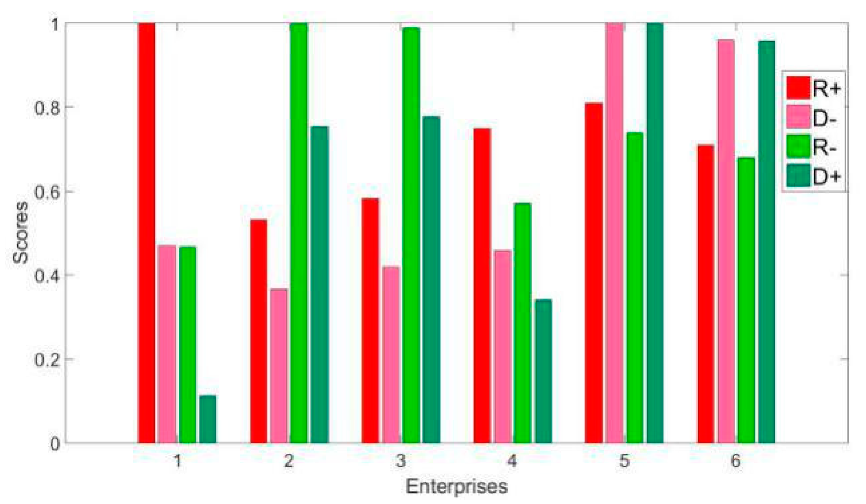
The positive and negative grey fuzzy integral vectors can be obtained by applying Equations (23) and (24) on the correlation matrix and the comprehensive weights vector which, respectively, were R + = [ 1.0000 ,   0.5314 ,   0.5824 ,   0.7486 ,   0.8085 ,   0.7103 ] and R = [ 0.4665 ,   1.0000 ,   0.9881 ,   0.5708 ,   0.7381 ,   0.6792 ] .
Step 6: Calculate fuzzy distance to ideal solution.
The positive and negative ideal solution distance vectors can be calculated by applying Equations (25), (26) on the standardized evaluation matrix and the comprehensive weights vector, which, respectively, were D + = [ 0.1119 ,   0.7536 ,   0.7771 ,   0.3408 ,   1.0000 ,   0.9583 ] and D = [ 0.4690 ,   0.3669 ,   0.4180 ,   0.4585 ,   1.0000 ,   0.9597 ] .
Step 7: Calculate the comprehensive proximity degree.
Normalize R + , R , D + , D according to Equation (27). Set the parameter p as 0.5, which means the importance of shape and distance is the same. The positive and negative comprehensive proximity degree vectors can be calculated by applying Equation (28) on the grey fuzzy integral vector and the ideal solution distance vector, which, respectively, were S + = [ 0.7345 ,   0.4491 ,   0.5002 ,   0.6036 ,   0.9043 ,   0.8350 ] and S = [ 0.2892 ,   0.8768 ,   0.8826 ,   0.4558 ,   0.8691 ,   0.8188 ] .
The final comprehensive evaluation vector can be obtained by aggregating the positive and negative comprehensive proximity degree vector according to Equation (29) which was C S = [ 0.7175 ,   0.3387 ,   0.3617 ,   0.5697 ,   0.5099 ,   0.5049 ] . The sequence of objects was 1 4 5 6 3 2 .
Intuitively, Figure 6 shows that enterprise 1 performed very well on all criteria; while enterprise 2 performed very badly on all criteria. Enterprise 4 performed averagely on criteria 1, 2, 4, and 5 but performed excellently on criterion 3. Enterprises 5, 6, and 3 all performed averagely and enterprise 5 performed slightly better than enterprise 6, and enterprise 6 performed slightly better than enterprise 3 on most criteria. The sequence coincided with our intuitionistic judgment.
The bar chart of R + ,   R ,   D + ,   and   D is depicted in Figure 7. It shows that the values of R + ,   R ,   D + ,   and   D were not coincident. If we concentrate on different aspects, we can obtain different evaluation results.

5.2. Comparisons and Sensitivity Analysis

To compare the effects of the proposed method with the existing methods, the result of GCE and TOPSIS is given below.
By standardizing w 0 , the weights of GCE can be obtained. The absolute correlation degree (ACD) can be calculated according to the weights and the positive correlation matrix. The ideal solution distance D T O P S I S + and D T O P S I S can be found by the standardized evaluation matrix. The relative closeness degree (RCD) can be obtained through D T O P S I S +   and D T O P S I S .
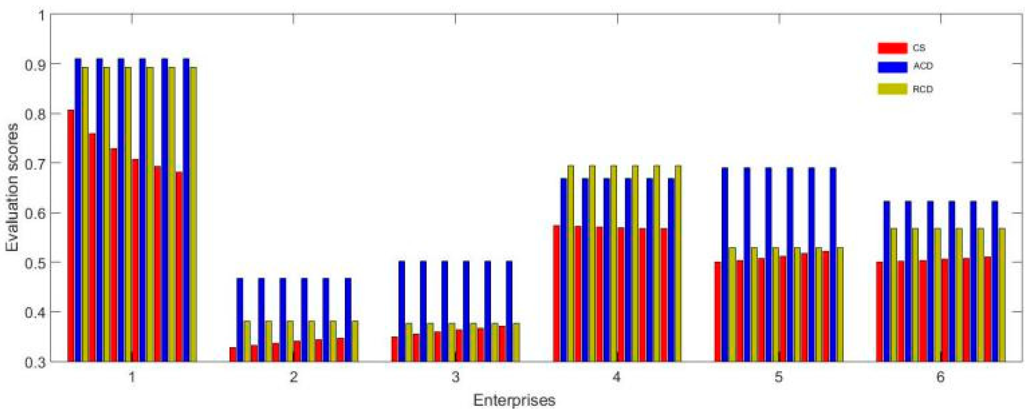
To carry out a sensitivity analysis of parameter p , a series of experiments was conducted and the value of p was between 0 and 1, and the interval was 0.2. The result is shown in Table 6 and Figure 8.

5.3. Result Analysis

Table 6 and Figure 8 show that the sequence sorted according to GCE was always 1 5 4 6 3 2 while the sequence sorted due to TOPSIS was always 1 4 6 5 3 2 . The result means that enterprise 4 is bad in terms of shape but good in terms of distance since it performed well on criterion 3 but badly on criteria 1 and 2. Enterprise 5 is bad in terms of distance, but good in terms of shape since it performed slightly better than average on most criteria, which is similar to enterprise 1.
The sequence sorted according to FGT is slightly related to parameter p . When p = 0 , the sequence was 1 4 5 6 2 3 . when p > 0 , the sequence was 1 4 5 6 3 2 . Enterprise 2 has slight advantages on distance, since it performed barely satisfactorily on criteria 4 and 5. However, its performance was instable. When the factor of shape is taken into consideration, enterprise 3 will be better than enterprise 2. Figure 8 clearly shows that the comprehensive evaluation value of enterprise 1 ( C S 1 ) obviously decreased, C S 4 slightly decreased, C S 2 , C S 3 , and C S 5 obviously increased, and C S 6 slightly increased with the increase of parameter p , i.e., the increase consideration of shape.
The result shows that the proposed method can reflect both the difference of shape and distance of objects, which overcomes the one-sidedness of the GCE method and TOPSIS method.

6. Conclusions

Generally speaking, the MCDM problems are essential in modern society for businesses and private individuals. The existing MCDM methods, such as GCE and TOPSIS, have some disadvantages which cannot take the interaction of criteria into consideration. In the view of this, a novel MCDM method that combines the GCE, TOPSIS, and fuzzy integral, called the fuzzy grey TOPSIS, was proposed to improve the deficiency mentioned above. The effectiveness of the proposed method was verified by the illustrative example of supplier evaluation of a collaborative manufacturing enterprise as well as some sensitivities.
There are some recommendations for future studies. One idea is to focus on other types of fuzzy numbers and correlation coefficients and even redefine them. We will compare them by conducting more experiments and refine the proposed method [85,86,87]. As such, hybridizing the proposed MCDM method with recent advances in heuristics and metaheuristics is another good continuation of this work [88,89,90,91,92,93].

Author Contributions

Conceptualization, G.T. and J.T.; Methodology, N.H. and Z.L.; Hardware and software, A.M.F.-F. and Z.Z.; Writing and validation, Y.F., Z.Z. and W.W.

Funding

This work was supported by the Science Fund for Creative Research Groups of National Natural Science Foundation of China (No. 51821093), the National Natural Science Foundation of China (Nos. 51935009 and 51775238), and Zhejiang Provincial Natural Science Foundation of China (No. LZ18E050001).

Acknowledgments

Sincere appreciation is extended to the reviewers of this paper for their helpful comments.

Conflicts of Interest

The authors declare no conflict of interest.

Notations and Nomenclature

A = { a 1 , a 2 , , a m } The objects set.
X = { x 1 , x 2 , , x n } The criterion set.
j ˜ i k The evaluation value of the i-th object on the k-th qualitative criterion in the form of fuzzy number,   i A , k { x k | x k   is   a   qualitative   criterion } . For the convenience, j ˜ a i x k is presented in a simplified form as j ˜ i k .
M i k 1 , M i k 2 , M i k 3 The numerical results of defuzzification of j ˜ i k through methods 1, 2, and 3.
J * = [ j 1 * j 1 n j m * j m n ] Numerical evaluation matrix of qualitative criteria.
j i k The evaluation value of the i-th object on the k-th criterion, i = 1 , 2 , , m , k = 1 , 2 , , n .
J = [ j 11 j 1 n j m 1 j m n ] Evaluation matrix.
c i k The standardized evaluation value of the i-th object on the k-th criterion, i = 1 , 2 , , m , k = 1 , 2 , , n .
C = [ c 11 c 1 n c m 1 c m n ] Standardized evaluation matrix.
C + = [ c 1 + , c 2 + , , c n + ] Positive ideal solution scheme.
C = [ c 1 , c 2 , , c n ] Negative ideal solution scheme.
ξ + = [ ξ 11 + ξ 1 n + ξ m 1 + ξ m n + ] Positive correlation matrix.
ξ = [ ξ 11 ξ 1 n ξ m 1 ξ m n ] Negative correlation matrix.
ω 1 = [ ω 1 1 , ω 2 1 , , ω n 1 ] Objective weights vector.
ω 2 = [ ω 1 2 , ω 2 2 , , ω n 2 ] Subjective weights vector.
Comprehensive weights vector.
λParameter of λ-fuzzy-measures.
ω Q The fuzzy measure of the subset Q of power set of X . For example, represents a set consisting of x 1 , x 3 ,   and   x 5 . For convenience, ω x 1 x 3 x 5 is presented in a simplified form as ω 135 .
Positive grey fuzzy integral vector.
R = [ R 1 , R 2 , , R m ] Negative grey fuzzy integral vector.
Positive fuzzy ideal solution distance.
Negative fuzzy ideal solution distance.
S + = [ S 1 + , S 2 + , , S m + ] Positive comprehensive proximity degree vector.
S = [ S 1 , S 2 , , S m ] Negative comprehensive proximity degree vector.
C S = [ C S 1 , C S 1 , , C S 1 ] Comprehensive evaluation vector.

References

  1. Gumus, S.; Egilmez, G.; Kucukvar, M.; Shin Park, Y. Integrating expert weighting and multi-criteria decision making into eco-efficiency analysis: The case of US manufacturing. J. Oper. Res. Soc. 2016, 67, 616–628. [Google Scholar] [CrossRef]
  2. Xue, Y.X.; You, J.X.; Zhao, X.; Liu, H.C. An integrated linguistic MCDM approach for robot evaluation and selection with incomplete weight information. Int. J. Prod. Res. 2016, 110, 1–16. [Google Scholar] [CrossRef]
  3. Shen, K.Y.; Hu, S.K.; Tzeng, G.H. Financial modeling and improvement planning for the life insurance industry by using a rough knowledge based hybrid MCDM model. Inf. Sci. 2017, 375, 296–313. [Google Scholar] [CrossRef]
  4. Govindan, K.; Kannan, D.; Shankar, M. Evaluation of green manufacturing practices using a hybrid mcdm model combining danp with promethee. Int. J. Prod. Res. 2015, 53, 1–28. [Google Scholar] [CrossRef]
  5. Liou, J.J.; Tamošaitienė, J.; Zavadskas, E.K.; Tzeng, G.H. New hybrid COPRAS-G MADM model for improving and selecting suppliers in green supply chain management. Int. J. Prod. Res. 2015, 263, 1–21. [Google Scholar] [CrossRef]
  6. Wang, Y.M.; Parkan, C. A preemptive goal programming method for aggregating OWA operator weights in group decision making. Inf. Sci. 2007, 177, 1867–1877. [Google Scholar] [CrossRef]
  7. Tsai, P.F.; Lin, F.M. An application of multi-attribute value theory to patient-bed assignment in hospital admission management: An empirical study. J. Healthc. Eng. 2014, 5, 439–456. [Google Scholar] [CrossRef] [PubMed]
  8. Torrance, G.W.; Boyle, M.H.; Horwood, S.P. Application of multi-attribute utility theory to measure social preferences for health states. Oper. Res. 1982, 30, 1043–1069. [Google Scholar] [CrossRef]
  9. Wang, X.; Chen, X.; Hu, H.; Yu, K.; Li, Z. Research on self-healing restoration strategy of urban power grid based on multi-agent technology. In 2011 International Conference on Advanced Power System Automation and Protection; IEEE: Piscatville, NJ, USA, 2011; pp. 1215–1218. [Google Scholar]
  10. Saaty, T.L. Decision making with the analytic hierarchy process. Int. J. Serv. Sci. 2008, 1, 83–98. [Google Scholar] [CrossRef]
  11. Cook, W.D. Data envelopment analysis: A comprehensive text with models, applications, references and DEA-solver software. J. Oper. Res. Soc. 2001, 52, 1408–1409. [Google Scholar]
  12. Boran, F.E.; Genç, S.; Kurt, M.; Akay, D. A multi-criteria intuitionistic fuzzy group decision making for supplier selection with TOPSIS method. Expert Syst. Appl. 2009, 36, 11363–11368. [Google Scholar] [CrossRef]
  13. Tian, G.D.; Zhang, H.H.; Feng, Y.; Jia, H.; Zhang, C.; Jiang, Z.; Li, Z.; Li, P. Operation patterns analysis of automotive components remanufacturing industry development in China. J. Clean. Prod. 2017, 64, 1363–1375. [Google Scholar] [CrossRef]
  14. Huang, K.; Chen, S.F.; Sun, Y.; Qi, X. Study and implementation on the grey comprehensive evaluation support system of ecocity. J. Southeast Univ. (Engl. Ed.) 2002, 18, 356–360. [Google Scholar]
  15. Gong, L.; Jin, C. Fuzzy comprehensive evaluation for carrying capacity of regional water resources. Water Resour. Manag. 2009, 23, 2505–2513. [Google Scholar] [CrossRef]
  16. Hopfield, J.J. Artificial neural networks. IEEE Circuits Devices Mag. 1988, 4, 3–10. [Google Scholar] [CrossRef]
  17. Pati, N.; Sahu, A.K.; Datta, S.; Mahapatra, S.S. Evaluation and selection of suppliers considering green perspectives: Comparative analysis on application of FMLMCDM and fuzzy-TOPSIS. Benchmarking 2016, 23, 1579–1604. [Google Scholar]
  18. Mousavi, S.M.; Torabi, S.A.; Tavakkoli-Moghaddam, R. A hierarchical group decision-making approach for new product selection in a fuzzy environment. Arab. J. Sci. Eng. 2013, 38, 3233–3248. [Google Scholar] [CrossRef]
  19. Mousavi, S.M.; Jolai, F.; Tavakkoli-Moghaddam, R.; Vahdani, B. A fuzzy grey model based on the compromise ranking for multi-criteria group decision making problems in manufacturing systems. J. Intell. Fuzzy Syst. 2013, 24, 819–827. [Google Scholar]
  20. Mousavi, S.M.; Vahdani, B.; Tavakkoli-Moghaddam, R.; Tajik, N. Soft computing based on a fuzzy grey compromise solution approach with an application to the selection problem of material handling equipment. Int. J. Comput. Integr. Manuf. 2014, 27, 547–569. [Google Scholar] [CrossRef]
  21. Mousavi, S.M.; Mirdamadi, S.; Siadat, A.; Dantan, J.; Tavakkoli-Moghaddam, R. An intuitionistic fuzzy grey model for selection problems with an application to the inspection planning in manufacturing firms. Eng. Appl. Artif. Intell. 2015, 39, 157–167. [Google Scholar] [CrossRef] [Green Version]
  22. Mousavi, S.M.; Vahdani, B. Cross-docking location selection in distribution systems: A new intuitionistic fuzzy hierarchical decision model. Int. J. Comput. Intell. Syst. 2016, 9, 91–109. [Google Scholar] [CrossRef]
  23. Hashemi, H.; Bazargan, J.; Mousavi, S.M. A compromise ratio method with an application to water resources management: An intuitionistic fuzzy set. Water Resour. Manag. 2013, 27, 2029–2051. [Google Scholar] [CrossRef]
  24. Shukla, V.; Auriol, G. Hipel, K.W. Multicriteria decision-making methodology for systems engineering. IEEE Syst. J. 2016, 10, 4–14. [Google Scholar] [CrossRef]
  25. Huang, E.; Zhang, S.; Lee, L.H.; Chew, E.P.; Chen, C.H. Improving analytic hierarchy process expert allocation using optimal computing budget allocation. IEEE Trans. Syst. Man Cybern. Syst. 2016, 46, 1140–1147. [Google Scholar] [CrossRef]
  26. Kuang, H.B.; Bashar, M.A.; Hipel, K.W.; Kilgour, D.M. Grey-based preference in a graph model for conflict resolution with multiple decision makers. IEEE Trans. Syst. Man Cybern. Syst. 2015, 45, 1254–1267. [Google Scholar] [CrossRef]
  27. Özpeynirci, Ö.; Özpeynirci, S.; Kaya, A. An interactive approach for multiple criteria selection problem. Compu. Oper. Res. 2017, 78, 154–162. [Google Scholar] [CrossRef]
  28. Zhou, Q.; Shi, P.; Liu, H.; Xu, S. Neural-network-based decentralized adaptive output-feedback control for large-scale stochastic nonlinear systems. IEEE Trans. Syst. Man Cybern. Part B Cybern. 2012, 42, 1608–1619. [Google Scholar] [CrossRef] [PubMed]
  29. Mohamed, A.A.M. An interactive Bi-criteria heuristic algorithm for the coherent system assembly. In 2014 IEEE International Conference on Industrial Engineering and Engineering Management; IEEE: Piscatville, NJ, USA, 2015; Volume 25, pp. 49–53. [Google Scholar]
  30. Liao, H.; Xu, Z.; Zeng, X.J. Hesitant fuzzy linguistic vikor method and its application in qualitative multiple criteria decision making. IEEE Trans. Fuzzy Syst. 2015, 23, 1343–1355. [Google Scholar] [CrossRef]
  31. Tehrani, A.F.; Cheng, W.W.; Hullermeier, E. Preference learning using the Choquet integral: The case of multipartite ranking. IEEE Trans. Fuzzy Syst. 2012, 20, 1102–1113. [Google Scholar] [CrossRef]
  32. Su, X.; Wu, L.; Shi, P.; Song, Y.D. H-infinity model reduction of takagi–sugeno fuzzy stochastic systems. IEEE Trans. Syst. Man Cybern. Part B Cybern. 2012, 42, 1574–1585. [Google Scholar]
  33. Meng, F.; Chen, X.; Zhang, Q. Induced generalized hesitant fuzzy Shapley hybrid operators and their application in multi-attribute decision making. Appl. Soft Comput. 2015, 28, 599–607. [Google Scholar] [CrossRef]
  34. Wu, Y.; Geng, S.; Xu, H.; Zhang, H. Study of decision framework of wind farm project plan selection under intuitionistic fuzzy set and fuzzy measure environment. Energy Convers. Manag. 2014, 87, 274–284. [Google Scholar] [CrossRef]
  35. Sugeno, M. Fuzzy measure and fuzzy integral. Trans. Soc. Instrum. Control Eng. 1972, 2, 218–226. [Google Scholar] [CrossRef]
  36. Mesiar, R.; Mesiarova-Zemenkova, A. Ahmad, K. Level-dependent Sugeno integral. IEEE Trans. Fuzzy Syst. 2009, 17, 167–172. [Google Scholar] [CrossRef]
  37. Hu, Y.C.; Chen, H.C. Choquet integral-based hierarchical networks for evaluating customer service perceptions on fast food stores. Expert Syst. Appl. 2010, 37, 7880–7887. [Google Scholar] [CrossRef]
  38. Wang, X.Z. Fuzzy Measure and Fuzzy Integral and Its Application in Classifier Technology; Science Publishing Company: Beijing, China, 2008. (In Chinese) [Google Scholar]
  39. He, Q.; Chen, J.F.; Yuan, X.Q.; Li, J. Choquet fuzzy integral aggregation based on g-lambda fuzzy measure. In 2007 International Conference on Wavelet Analysis and Pattern Recognition; IEEE: Piscatville, NJ, USA, 2007; pp. 98–102. [Google Scholar]
  40. Dymova, L.; Sevastjanov, P.; Tikhonenko, A. An interval type-2 fuzzy extension of the topsis method using alpha cuts. Knowl. Based Syst. 2015, 83, 116–127. [Google Scholar] [CrossRef]
  41. Xia, X.; Sun, Y.; Wu, K.; Jiang, Q. Optimization of a straw ring-die briquetting process combined analytic hierarchy process and grey correlation analysis method. Fuel Process. Technol. 2016, 152, 303–309. [Google Scholar] [CrossRef]
  42. Bouzarour-Amokrane, Y.; Tchangani, A.; Peres, F. A bipolar consensus approach for group decision making problems. Expert Syst. Appl. 2015, 42, 1759–1772. [Google Scholar] [CrossRef] [Green Version]
  43. Tchangani, A.P. Bipolar aggregation method for fuzzy nominal classification using Weighted Cardinal Fuzzy Measure (WCFM). J. Uncertain Syst. 2013, 7, 138–151. [Google Scholar]
  44. Zhang, H.H.; Peng, Y.; Hou, L.; Tian, G.D.; Li, Z.W. A hybrid multi-objective optimization approach for energy-absorbing structures in train collisions. Inf. Sci. 2019, 481, 491–506. [Google Scholar] [CrossRef]
  45. Mousavi-Nasab, S.H.; Sotoudeh-Anvari, A. A new multi-criteria decision making approach for sustainable material selection problem: A critical study on rank reversal problem. J. Clean. Prod. 2018, 182, 466–484. [Google Scholar] [CrossRef]
  46. Hassan, M.N.; Hawas, Y.E.; Ahmed, K. A multi-dimensional framework for evaluating the transit service performance. Trans. Res. Part A Policy Pract. 2013, 50, 47–61. [Google Scholar] [CrossRef]
  47. Kazançoğlu, Y.; Kazançoğlu, İ. Benchmarking service quality performance of airlines in Turkey. Eskişehir Osman. Üniversitesi İktis. ve İdari Bilim. Derg. 2013, 8, 59–91. [Google Scholar]
  48. Bagočius, V.; Zavadskas, E.K.; Turskis, Z. Selecting a location for a liquefied natural gas terminal in the Eastern Baltic Sea. Transport 2014, 29, 69–74. [Google Scholar] [CrossRef]
  49. Yayla, A.Y.; Oztekin, A.; Gumus, A.T.; Gunasekaran, A. A hybrid data analytic methodology for 3PL transportation provider evaluation using fuzzy multi-criteria decision making. Int. J. Prod. Res. 2015, 53, 6094–6113. [Google Scholar] [CrossRef]
  50. John, A.; Yang, Z.; Riahi, R.; Wang, J. Application of a collaborative modelling and strategic fuzzy decision support system for selecting appropriate resilience strategies for seaport operations. J. Traffic Trans. Eng. 2014, 1, 159–179. [Google Scholar] [CrossRef] [Green Version]
  51. Shanian, A.; Savadogo, O. TOPSIS multiple-criteria decision support analysis for material selection of metallic bipolar plates for polymer electrolyte fuel cell. J. Power Source 2006, 159, 1095–1104. [Google Scholar] [CrossRef]
  52. Olson, D.L. Comparison of weights in TOPSIS models. Math. Comput. Model. 2004, 40, 721–727. [Google Scholar] [CrossRef]
  53. Deng, H.; Yeh, C.H.; Willis, R.J. Inter-company comparison using modified TOPSIS with objective weights. Comput. Oper. Res. 2000, 27, 963–973. [Google Scholar] [CrossRef]
  54. Buyukozkan, G.; Cifci, G. A combined fuzzy AHP and fuzzy TOPSIS based strategic analysis of electronic service quality in healthcare industry. Expert Syst. Appl. 2012, 39, 2341–2354. [Google Scholar] [CrossRef]
  55. Zavadskas, E.K.; Susinskas, S.; Daniunas, A.; Turskis, Z.; Sivilevicius, H. Multiple criteria selection of pile-column construction technology. J. Civ. Eng. Manag. 2012, 18, 834–842. [Google Scholar] [CrossRef]
  56. Buyukozkan, G.; Cifci, G. A novel hybrid MCDM approach based on fuzzy DEMATEL, fuzzy ANP and fuzzy TOPSIS to evaluate green suppliers. Expert Syst. Appl. 2012, 39, 3000–3011. [Google Scholar] [CrossRef]
  57. Zavadskas, E.K.; Turskis, Z.; Volvaciovas, R.; Kildiene, S. Multi-criteria assessment model of technologies. Stud. Inform. Control 2013, 22, 249–258. [Google Scholar] [CrossRef]
  58. Zavadskas, E.K.; Turskis, Z.; Tamosaitiene, J. Risk assessment of construction projects. J. Civ. Eng. Manag. 2010, 16, 33–46. [Google Scholar] [CrossRef]
  59. Yazdani, M.; Payam, A.F. A comparative study on material selection of micro-electromechanical systems electrostatic actuators using Ashby, VIKOR and TOPSIS. Mater. Des. 2015, 65, 328–334. [Google Scholar] [CrossRef]
  60. Greco, S.; Matarazzo, B.; Slowinski, R. Rough sets theory for multicriteria decision analysis. Eur. J. Oper. Res. 2001, 129, 1–47. [Google Scholar] [CrossRef]
  61. Diakoulaki, D.; Karangelis, F. Multi-criteria decision analysis and cost-benefit analysis of alternative scenarios for the power generation sector in Greece. Renew. Sustain. Energy Rev. 2007, 11, 716–727. [Google Scholar] [CrossRef]
  62. Pohekar, S.; Ramachandran, M. Application of multi-criteria decision making to sustainable energy planning-a review. Renew. Sustain. Energy Rev. 2004, 8, 365–381. [Google Scholar] [CrossRef]
  63. Tian, G.; Zhang, H.; Feng, Y.; Wang, D.; Peng, Y.; Jia, H. Green decoration materials selection under interior environment characteristics: a grey-correlation based hybrid MCDM Method. Renew. Sustain. Energy. Rev. 2018, 81, 682–692. [Google Scholar] [CrossRef]
  64. Hashemi, S.H.; Karimi, A.; Aghakhani, N.; Kalantar, P. A grey-besed carbon management model for green supplier selection. In 2013 IEEE International Conference on Grey systems and Intelligent Services (GSIS); IEEE: Piscatville, NJ, USA, 2014; Volume 26, pp. 402–405. [Google Scholar]
  65. Sarucan, A.; Baysal, M.E.; Kahraman, C.; Engin, O. A hierarchy grey relational analysis for selecting the renewable electricity generation technologies. Lect. Notes Eng. Comput. Sci. 2011, 2, 1149–1154. [Google Scholar]
  66. Ebrahimi, M.; Keshavarz, A. Prime mover selection for a residential micro CCHP by using two multi-criteria decision-making methods. Energy Build. 2012, 55, 322–331. [Google Scholar] [CrossRef]
  67. Wang, J.; Zhang, C.; Jing, Y.; Zheng, G. Using the fuzzy multi-criteria model to select the optimal cool storage system for air conditioning. Energy Build. 2008, 40, 2059–2066. [Google Scholar] [CrossRef]
  68. Wang, J.; Zhang, C.; Zhao, J. Review on multi-criteria decision analysis aid in sustainable energy decision-making. Renew. Sustain. Energy Rev. 2009, 13, 2263–2278. [Google Scholar] [CrossRef]
  69. Lee, W.; Lin, Y. Evaluating and ranking energy performance of office buildings using grey relational analysis. Energy 2011, 36, 2551–2556. [Google Scholar] [CrossRef]
  70. Abhang, L.B.; Hameedullah, M. Determination of optimum parameters for multi-performance characteristics in turning by using grey relational analysis. Int. J. Adv. Manuf. Technol. 2012, 63, 13–24. [Google Scholar] [CrossRef] [Green Version]
  71. Aydin, N.; Celik, E.; Gumus, A.T. A hierarchical customer satisfaction framework for evaluating rail transit systems of Istanbul. Trans. Res. Part A Policy Pract. 2015, 77, 61–81. [Google Scholar] [CrossRef]
  72. Celik, E.; Aydin, N.; Gumus, A.T. A multiattribute customer satisfaction evaluation approach for rail transit network: a real case study for Istanbul, Turkey. Transp. Policy 2014, 36, 283–293. [Google Scholar] [CrossRef]
  73. Feng, Y.; Zhou, M.; Tian, G.; Li, Z.; Zhang, Z.; Zhang, Q.; Tan, J. Target disassembly sequencing and scheme evaluation for CNC machine tools using improved multiobjective ant colony algorithm and fuzzy integral. IEEE Trans. Syst. Man Cybern. Syst. 2018. [Google Scholar] [CrossRef]
  74. Tian, G.; Hao, N.; Zhou, M.; Pedrycz, W.; Zhang, C.; Ma, F.; Li, Z. Fuzzy Grey Choquet Integral for Evaluation of Multicriteria Decision Making Problems with Interactive and Qualitative Indices. IEEE Trans. Syst. Man Cybern. Syst. 2019. [Google Scholar] [CrossRef]
  75. Wu, S.L.; Liu, Y.T.; Hsieh, T.Y.; Lin, Y.Y.; Chen, C.Y.; Chuang, C.H.; Lin, C.T. Fuzzy integral with particle swarm optimization for a Motor-Imagery-Based Brain-Computer interface. IEEE Trans. Fuzzy Syst. 2017, 25, 21–28. [Google Scholar] [CrossRef]
  76. Zhu, L.; Zhu, C.X.; Zhang, X.Z. Method for hesitant fuzzy multi-attribute decision making based on rough sets. Control Decis. 2014, 29, 1335–1339. [Google Scholar]
  77. Fu, C.; Zhao, J. Multiple attribute making method based on hesitation institution fuzzy number. Syst. Eng. 2014, 32, 131–136. [Google Scholar]
  78. Lin, Y.; Lee, P.; Chang, T.; Ting, H. Multi-attribute group decision making model under the condition of uncertain information. Autom. Constr. 2008, 17, 792–797. [Google Scholar] [CrossRef]
  79. Zhang, G.; He, L.H. Method based on fuzzy integral about construction and optimization of supply chain networks. Comput. Eng. Appl. 1983, 9, 173–175. [Google Scholar]
  80. Yan, T.; Feng, S.; Bi, X.L. Chang, L. Grey correlation analysis and applications of drill stem failure in drilling engineering. In 2010 Seventh International Conference on Fuzzy Systems and Knowledge Discovery; IEEE: Piscatville, NJ, USA, 2010; Volume 4, pp. 1699–1702. [Google Scholar]
  81. Zhu, J. Study on Measuring and Evaluating Product Innovation of Small and Medium Enterprises; Harbin University of Science and Technology: Harbin, China, 2003. (In Chinese) [Google Scholar]
  82. Delgado, A.; Romero, I. Environmental conflict analysis using an integrated grey clustering and entropy-weight method: A case study of a mining project in Peru. Environ. Model. Softw. 2016, 77, 108–121. [Google Scholar] [CrossRef]
  83. Delgado, M.; Herrera, F.; Herrera-Viedma, E.; Martinez, L. Combining numerical and linguistic information in group decision making. Inf. Sci. 1998, 107, 177–194. [Google Scholar] [CrossRef]
  84. Herrera, F.; Martinez, L. An approach for combining linguistic and numerical information based on the 2-tuple fuzzy linguistic representation model in decision-making. Int. J. Uncertain. Fuzziness Knowl. Based Syst. 2011, 8, 539–562. [Google Scholar] [CrossRef]
  85. Liu, Z.; Liu, Y.; He, B.J.; Xu, W.; Jin, G.; Zhang, X. Application and suitability analysis of the key technologies in nearly zero energy buildings in China. Renew. Sustain. Energy. Rev. 2019, 101, 329–345. [Google Scholar] [CrossRef]
  86. Tian, G.; Zhou, M.; Li, P. Disassembly sequence planning considering fuzzy component quality and varying operational cost. IEEE Trans. Autom. Sci. Eng. 2018, 15, 748–760. [Google Scholar] [CrossRef]
  87. Fard, A.F.; Hajiaghaei-Keshteli, M. Red Deer Algorithm (RDA); a new optimization algorithm inspired by Red Deers’ mating. In International Conference on Industrial Engineering; IEEE: Piscatville, NJ, USA, 2016; Volume 12, pp. 331–342. [Google Scholar]
  88. Gu, C.; Li, Z.W.; Wu, N.Q.; Khalgui, M.; Qu, T.; Al-Ahmari, A. Improved multi-step look-ahead control policies for automated manufacturing systems. IEEE Access 2018, 6, 68824–68838. [Google Scholar] [CrossRef]
  89. Fathollahi-Fard, A.M.; Hajiaghaei-Keshteli, M.; Tavakkoli-Moghaddam, R. The social engineering optimizer (SEO). Eng. Appl. Artif. Intell. 2018, 72, 267–293. [Google Scholar] [CrossRef]
  90. Hajiaghaei-Keshteli, M.; Fathollahi-Fard, A.M. A set of efficient heuristics and metaheuristics to solve a two-stage stochastic bi-level decision-making model for the distribution network problem. Comput. Ind. Eng. 2018, 123, 378–395. [Google Scholar] [CrossRef]
  91. Fathollahi-Fard, A.M.; Hajiaghaei-Keshteli, M.; Tavakkoli-Moghaddam, R. A bi-objective green home health care routing problem. J. Clean. Prod. 2018, 200, 423–443. [Google Scholar] [CrossRef]
  92. Feng, Y.; Gao, Y.; Tian, G.; Li, Z.; Hu, H.; Zheng, H. Flexible process planning and end-of-life decision-making for product recovery optimization based on hybrid disassembly. IEEE Trans. Autom. Sci. Eng. 2019, 16, 311–326. [Google Scholar] [CrossRef]
  93. Tian, G.; Ren, Y.; Feng, Y.; Zhou, M.; Zhang, H.; Tan, J. Modeling and Planning for Dual-Objective Selective Disassembly Using AND/OR Graph and Discrete Artificial Bee Colony. IEEE Trans. Ind. Inform. 2019, 15, 2456–2468. [Google Scholar] [CrossRef]
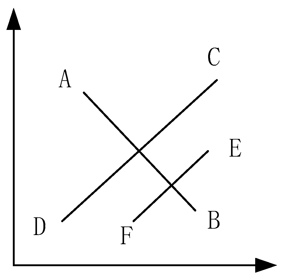
Figure 1. Technique for order preference by similarity to an ideal solution (TOPSIS) failed conditions.
Applsci 09 03770 g001
Figure 2. Grey comprehensive evaluation (GCE) failed conditions.
Applsci 09 03770 g002
Figure 3. The flow chart of Grey Fuzzy TOPSIS.
Applsci 09 03770 g003
Figure 4. Supplier evaluation criterion system.
Applsci 09 03770 g004
Figure 5. The 3-dimensional histograms of J .
Applsci 09 03770 g005
Figure 6. The 3-dimensional histograms of C .
Applsci 09 03770 g006
Figure 7. Bar chart of R + ,   R ,   D + ,   D .
Applsci 09 03770 g007
Figure 8. The result of sensitivity analysis.
Applsci 09 03770 g008
Table 1. Review of the technique for order preference by similarity to an ideal solution (TOPSIS).
Typical ReferenceTool TypeAdvantageLimitation
Hassan et al. [46]TOPSISFlexible frameworkExperts have too many rights
Kazançoğlu et al. [47]Fuzzy TOPSISSimpleHard to describe complex systems
Bagočius et al. [48]TOPSIS and COPRAS, SAWVarious comparisonHard to describe complex systems
Yayla et al. [49]Fuzzy TOPSIS and Fuzzy-AHPMore realistic and reliableComplicated and abstract models
John et al. [50]Fuzzy TOPSIS and Fuzzy-AHPMore realistic and reliableComplicated and abstract models
Shanian and Savadogo [51]Ordinary and Block TOPSISSimple and fastComplicated
Olson [52]TOPSISSimple and fastNot accurate enough
Deng et al. [53]Weighted Euclidean distances TOPSISSimple and directNot accurate enough
Buyukozkan and Cifci [54,55]Fuzzy AHP and fuzzy TOPSISSolving the uncertainty problem of score evaluationHard to describe complex systems
Zavadskas et al. [56,57,58]TOPSIS, COPRAS, and ARASAggregate both quantitative and qualitative criteriaComplicated and abstract models
Yazdani and Payam [59]Ashby, VIKOR, and TOPSISVarious comparisonComplicated and abstract models
Table 2. Literature review of grey evaluation methods.
Typical ReferenceTool TypeAdvantageLimitation
Greco et al. [60]Rough sets theory and MCDAThe use of the decision rule model and the capacityToo simple
Diakoulaki and Karangelis [61]MCDA and CBABroadening the evaluation perspectiveEach method is often disputed
Pohekar and Ramachandran [62]MCDM, PROMETHEE, and ELECTRECompare in a variety of waysThinking not deep enough
Tian et al. [63]GRA and AHPSimple and fastDependent on index selection
Hashemi et al. [64]Improved grey relational analysisNovel and convenientHard to describe complex systems
Sarucan et al. [65]AHP and GRAMore realistic and reliableComplicated and abstract models
Ebrahimi and Keshavarz [66]FA and GIATwo-phase comparison results are consistentComplicated and abstract models
Wang et al. [67,68]Fuzzy and weighting methodMore realistic and reliableTheory still flawed
Lee and Lin [69]GRAReasonable and efficientThe reference factor is not enough
Abhang and Hameedullah [70]Grey relational analysisEffectively improve accuracyComplicated and abstract models
Table 3. Literature review of fuzzy integral and fuzzy set.
Typical ReferenceTool TypeAdvantageLimitation
Aydin et al. [71]Fuzzy-AHP, Choquet integral and trapezoidal fuzzy setsRealistic and reliableComplicated and abstract models
Celik et al. [72]VIKOR and interval type-2 fuzzy setsEffectively improve accuracyComplicated and abstract models
Feng et al. [73]Fuzzy integralConvenientComplicated
Tian et al. [74]Choquet fuzzy integralEffectively improve accuracyComplicated
Wu et al. [75]Fuzzy Integral with Particle Swarm OptimizationSolving the uncertainty problemDependent on index selection
Zhu et al. [76]Fuzzy multi-attribute decision makingNovel and convenientDependent on index selection
Fu and Zhao [77]Hesitation institution fuzzy numberMore realistic and reliableComplicated and abstract model
Lin et al. [78]TOPSIS and aggregation approachEfficient and robust, realistic and reasonableComplicated and abstract model
Table 4. Mapping rules of linguistic variables and fuzzy numbers.
Superb (S)(0.8, 0.9, 0.9)
Good (G)(0.6, 0.7, 0.8)
Normal (N)(0.4, 0.5, 0.6)
Bad (B)(0.2, 0.3, 0.4)
Terrible (T)(0.1, 0.1, 0.2)
Table 5. Fuzzy measures.
SetsMeasuresSetsMeasuresSetsMeasures
10.210320.406930.2119
40.240450.2405120.5722
130.3988140.4241150.4242
230.5734240.5958250.5959
340.4255350.4256450.4504
1230.72031240.74021250.7402
1340.58881350.58881450.6109
2340.74132350.74132450.7609
3450.612112340.869612350.8696
12450.887013450.754723450.8880
123451.0000
where 1, 2, 3, 4 represent the sets of x 11 , x 12 , x 13 and x 14 , respectively (Similarly hereinafter).
Table 6. The result of sensitivity analysis.
pA1A2A3A4A5A6Sequence
CS00.80730.32740.34980.57370.50000.50031,4,6,5,3,2
ACD00.90970.46770.50220.66840.69070.62281,5,4,6,3,2
RCD00.89290.38070.37690.69490.52860.56851,4,6,5,2,3
CS0.20.75880.33240.35500.57180.50370.50201,4,5,6,2,3
ACD0.20.90970.46770.50220.66840.69070.62281,5,4,6,3,2
RCD0.20.89290.38070.37690.69490.52860.56851,4,6,5,2,3
CS0.40.72860.33680.35960.57040.50770.50391,4,5,6,3,2
ACD0.40.90980.46770.50220.66840.69070.62281,5,4,6,3,2
RCD0.40.89290.38070.37690.69490.52860.56851,4,6,5,2,3
CS0.60.70810.34060.3640.56920.51220.50601,4,5,6,3,2
ACD0.60.90980.46770.50220.66840.69070.62281,5,4,6,3,2
RCD0.60.89290.38070.37690.69490.52860.56851,4,6,5,2,3
CS0.80.69320.34400.36750.56820.51720.50841,4,5,6,3,2
ACD0.80.90980.46770.50220.66840.69070.62281,5,4,6,3,2
RCD0.80.89290.38070.37690.69490.52860.56851,4,6,5,2,3
CS10.68190.34700.37080.56740.52280.51121,4,5,6,3,2
ACD10.90980.46770.50220.66840.69070.62281,5,4,6,3,2
RCD10.89290.38070.37690.69490.52860.56851,4,6,5,2,3