FnnmOS-ELM: A Flexible Neural Network Mixed Online Sequential Elm

Abstract

The learning speed of online sequential extreme learning machine (OS-ELM) algorithms is much higher than that of convolutional neural networks (CNNs) or recurrent neural network (RNNs) on regression and simple classification datasets. However, the general feature extraction of OS-ELM makes it difficult to conveniently and effectively perform classification on some large and complex datasets, e.g., CIFAR. In this paper, we propose a flexible OS-ELM-mixed neural network, termed as fnnmOS-ELM. In this mixed structure, the OS-ELM can replace a part of fully connected layers in CNNs or RNNs. Our framework not only exploits the strong feature representation of CNNs or RNNs, but also performs at a fast speed in terms of classification. Additionally, it avoids the problem of long training time and large parameter size of CNNs or RNNs to some extent. Further, we propose a method for optimizing network performance by splicing OS-ELM after CNN or RNN structures. Iris, IMDb, CIFAR-10, and CIFAR-100 datasets are employed to verify the performance of the fnnmOS-ELM. The relationship between hyper-parameters and the performance of the fnnmOS-ELM is explored, which sheds light on the optimization of network performance. Finally, the experimental results demonstrate that the fnnmOS-ELM has a stronger feature representation and higher classification performance than contemporary methods.

1. Introduction

Classification tasks on various datasets have become a hot topic over the past decades. The accuracy of classification depends on two aspects: feature representation and classifier’s discriminability. Convolutional neural network (CNNs) [1] and many other network models are derived for feature extraction, which can directly take image data as input with their unique fine-grained feature extraction method without manual image preprocessing and other additional complex operations [2]. Recurrent neural networks (RNNs) [3] can remember the previous information and have more advantages over other network models in continuous, context-related, and feature extraction-related tasks, such as speech recognition. Similar to CNNs and RNNs, other types of neural networks have their own advantages in feature extraction, and great achievements have been made in recent studies [4,5,6,7].

In terms of classification, full connection layers play a major role in CNNs- or RNNs-based classifiers that use the back-propagation (BP) [8] algorithm to train networks. Previous studies have shown that the BP method is very sensitive to local minima, and overmuch training could lead to a decline in generalizability [9]. In addition, the repeated adjustment of the learning rate during the training process causes efficiency issues in research. The extreme learning machine (ELM) method [10,11,12,13,14] has been proven to be a fast and effective classification algorithm, which can be used to train multi-hidden layers feed-forward neural networks. Each hidden layer can be trained by a single-layer ELM. The whole network can be regarded as a single-layer ELM without adjusting the hidden layer nodes used for clustering, regression, and classification. The online sequential ELM (OS-ELM) [15], a fast and accurate online sequential learning algorithm, is suitable for single hidden layer feedforward networks (SLFNs) with additive or radial basis function (RBF) [11] hidden nodes in a unified framework. The OS-ELM is superior to other sequential learning algorithms and exhibits a superior generalizability with a relatively small number of training steps in real-world benchmark regression, classification, and time-series problems.

With the wide application of deep learning [16,17], the datasets are becoming increasingly more complex, which not only requires the classifier to have a good ability to distinguish and extract features, but also requires the algorithm to classify quickly and accurately. Although CNNs and RNNs have excellent feature representation, when the computing resources are limited, they take too long time for training model to achieve accurate classification [18,19,20]. On the other hand, the OS-ELM has high training and classification speed yet poor feature representation. Therefore, we propose a flexible neural networks mixed OS-ELM (fnnmOS-ELM) in this paper, which uses CNNs or RNNs as feature extractors and employs the OS-ELM as a classifier. Undoubtedly, when to tackle more complex CNNs, optimizing the original network structure could be more suitable than modifying it. Then we propose a method for using fnnmOS-ELM as an optimiser. In short, we propose a fnnmOS-ELM by fully combining the advantages of CNNs, RNNs, and OS-ELM. The main intellectual contributions can be summarized as follows.

(1)

The proposed fnnmOS-ELM fully exploits the feature representation of CNNs and RNNs with different datasets and makes use of the excellent classification characteristics of OS-ELM.

(2)

We extend the application of OS-ELM to more datasets, and our studies also show that fnnmOS-ELM can optimize the network performance of CNNs or RNNs without changing the original network structure.

(3)

We explore the effects of various hyper-parameters on the performance of the model in the mixed structure in detail and explain how to improve the performance of the model by adjusting these parameters.

The remainder of this paper is organized as follows. Section 2 gives an overview of the related work. Section 3 deals with the mathematical principles, network structure, and training process of the fnnmOS-ELM model. The experimental design, test results, as well as analysis of the proposed model on some classification datasets are provided in Section 4. Finally, a summary and ongoing work are offered in Section 5.

2. Related Work

In the past decades, researchers have conducted substantial research on SLFNs and applied them to a range of fields [21,22,23,24,25,26]. The BP algorithm plays a fundamental role in SLFNs research, and many algorithms are derived from it, such as stochastic gradient descent BP (SGBP) [8] and the recursive Levenberg-Marquardt algorithm [27]. These studies show that the BP is essentially a batch learning algorithm. In applications to deep neural networks, the use of the gradient descent algorithm leads to an excessively long training time [28]. Furthermore, in some sequential learning applications, excessively fast arrival of training data causes many problems.

Some studies have proved that SLFNs can learn accurately even if they use random weights and hidden layer biases [29,30], and in the meantime, can lead to fairly high training speeds. Huang et al. [10,11,12,13,14] proposed the ELM method, where they rigorously proved that the input weights and hidden layer biases of SLFNs can be randomly assigned. The problem of solving single hidden layer feedforward neural network is transformed into one of solving a linear system. The parameters of hidden layer nodes are given randomly or artificially without adjustment. The whole learning process only involves calculating the output weight by generalized inverse of matrices [31] without iterative training. The ELM is widely used in both binary classification [32,33,34] and multi-classification problems [35]. In real applications, the training data may arrive chunk-by-chunk or one-by-one, but the ELM usually needs a complete and definite dataset for training. Thus, the ELM is trained in a time-consuming manner, i.e., whenever a batch of new data arrives, the whole dataset needs to be trained.

To solve the above-mentioned problems, Liang et al. [15] proposed an OS-ELM, which is an online sequential learning algorithm for SLFNs with additive or RBF hidden nodes in a unified framework. For each batch or data, only the current new data is considered, while the old already-trained data will be ignored, so the OS-ELM solves the training problem required for data update. In this algorithm, additive nodes can be arbitrarily-bounded nonconstant piecewise continuous functions, the RBF nodes activation functions can be any integrable piecewise continuous function, and the output weight is determined only according to the latest data arrived sequentially. In the scope of regression, classification, and time series prediction, the OS-ELM is much faster than CNNs, BPs, and other batch-trained neural networks, which greatly improves the training speed and reduces the parameter size.

However, when dealing with more complex datasets, such as the CIFAR-100 dataset, the OS-ELM has several drawbacks. On the one hand, with randomly selected input weights, the OS-ELM has no advantage in feature representation and its robustness and stability is hardly guaranteed. On the other hand, by only learning the output layer weights, the OS-ELM is unable to achieve the desired results when it comes to regression and classification tasks that require deep neural networks. Therefore, it is usually necessary to increase the size of the training datasets, to increase the hidden layer nodes, or to change its original networks structure [36]. Huang et al. [37] studied the general architecture of locally connected ELM, and proposed local receptive fields based on ELM (ELM-LRF). Random convolutional nodes and a pooling structure were implemented in their studies, and they used the close relationship between local receptive fields and random hidden neurons to reduce the error rate and increase the learning speed on the NORB dataset. However, different types of local receptive fields and combinatorial nodes can have different effects on performance, and it is difficult to find the most appropriate type. At the same time, they only employed local receptive fields and do not fully utilized the feature extraction capability of convolutional layers. Duan et al. [38] introduced a hybrid deep learning CNN-ELM method. By combining CNN and ELM in a hybrid recognition architecture, they exploited the excellent feature representation of CNN and the fast inference speed of ELM. Good results were achieved in age and gender classification tasks but they adopted different dropout measures to limit the risk of overfitting, increasing the complexity of training. Furthermore, the two methods mentioned above are based on ELM, which adopts non-online sequential learning during training, and the whole dataset needs to be trained when a batch of new data arrives.

This paper proposes a network structure fnnmOS-ELM that mixes CNNs and RNNs with OS-ELM. The OS-ELM can flexibly replace some layers of the classifier network in CNNs and RNNs and is used together with the CNNs and RNNs structures as an optimiser. The fnnmOS-ELM model uses online sequential learning, and it makes full use of the feature representation of CNNs and RNNs, significantly reducing the training steps and parameter size. As opposed to OS-ELM, the fnnmOS-ELM has powerful feature representation and better adaptability to a variety of datasets. In contrast to CNNs and RNNs, it solves the problems of slow training and inference. Unlike the CNN-ELM model, we adopt the online sequential learning method, and the whole dataset does not need to be trained when a batch of new data arrives. In terms of network mixing, the more flexible fnnmOS-ELM can replace any layer in CNNs and RNNs classifier networks, and directly uses the OS-ELM as an optimiser.

3. Proposal and Implementation of FnnmOS-ELM

3.1. Proposal of FnnmOS-ELM

The ELM randomly selects the weights of the input layer and the biases of the hidden layer and uses the Moore-Penrose generalized inverse [31] to calculate the output weights. On this basis, OS-ELM uses online learning to update the output weights with one-by-one or chunk-by-chunk data samples. We propose the fnnmOS-ELM based on the OS-ELM.

For $N_0$ samples $\left(X,T_0\right)$, $X$ is the input vector and $T_0$ is the target vector, which is given by

$${\mathrm{T}}_0={\left[\begin{array}{c}{\mathrm{t}}_1^{\mathrm{T}}\\ ⋮\\ {\mathrm{t}}_{{\mathrm{N}}_0}^{\mathrm{T}}\end{array}\right]}_{{\mathrm{N}}_0\times \mathrm{L}},$$

(1)

where $L$ is the label dimension of a single data point. Typically, $L$ usually represents a category in a classification problem.

Let ${\mathrm{Net}}_n$ be a pre-trained network, where $n$ indexes over the network layers. Here, we consider $Y_i$ to be the $i$-th layer output of the neural network, where $i=0,1,\dots ,n$. The data used for online learning is a batch or a sample. In this paper, we use a batch. $D$ is the batch size, and the output $Y_i$ is divided into $Z$ batches, i.e., $Y_{iz}$ For the first batch, $Z=0$, and

$$Y_{i0}={\left[\begin{array}{ccc}{y}_{00}& \dots & y_{0M}\\ ⋮& \ddots & ⋮\\ y_{D0}& \dots & y_{DM}\end{array}\right]}_{D\times M},$$

(2)

where $M$ is the output dimension of a sample in the $i$-th neural network. With random weights $w_i$ and biases $b_i$,

$$W_i={\left[\begin{array}{ccc}{w}_{00}& \cdots & w_{0S}\\ ⋮& \ddots & ⋮\\ w_{M0}& \cdots & w_{MS}\end{array}\right]}_{M\times S},$$

(3)

$$b_i={\left[\begin{array}{c}{b}_{i0}\\ ⋮\\ b_{iD}\end{array}\right]}_{D\times 1},$$

(4)

where $S$ is the number of fnnmOS-ELM hidden layer nodes. The output matrix of the hidden layer is $H_0$, which can be written as

$$H_0=g\left(Y_{i0}·W_i+b_i\right),$$

(5)

where $g()$ is the activation function. We formulate $H_0$ as

$$H_0={\left[\begin{array}{ccc}{h}_{00}& \cdots & h_{0S}\\ ⋮& \ddots & ⋮\\ h_{D0}& \cdots & h_{DS}\end{array}\right]}_{D\times S}.$$

(6)

Then, the output matrix ${\beta }^{\left(0\right)}$ is

$${\beta }^{\left(0\right)}={\left[\begin{array}{ccc}{\beta }_{00}& \cdots & {\beta }_{0L}\\ ⋮& \ddots & ⋮\\ {\beta }_{S0}& \cdots & {\beta }_{SL}\end{array}\right]}_{S\times L},$$

(7)

When $\left|\right|H_0\beta -T_0\left|\right|$ is a minimum, ${\beta }^{\left(0\right)}$ can be written as

$${\beta }^{\left(0\right)}=K_0^{-1}{H}_0^T{T}_0,$$

(8)

where $K_0=H_0^T{H}_0$. When the next $Y_{i1}$ batch arrives $\left(Z=1\right)$, the problem is reformed as minimizing

$$\left|\right|\left[\begin{array}{c}{H}_0\\ H_1\end{array}\right]{\beta }^{\left(1\right)}-\left[\begin{array}{c}{T}_0\\ T_1\end{array}\right]\left|\right|,$$

(9)

According to the results of Liang et al. [15], ${\beta }^{\left(1\right)}$ can be expressed as ${\beta }^{\left(0\right)}$. Thus, the recursive formula of online learning can be written as

$$\begin{array}{c}{P}_{k+1}=P_k-P_k{H}_{k+1}^T{\left(I+H_{k+1}{P}_k{H}_{k+1}^T\right)}^{-1}{H}_{k+1}{P}_k\\ {\beta }^{\left(k+1\right)}={\beta }^{\left(k\right)}+P_{k+1}{H}_{k+1}^T\left(T_{k+1}-H_{k+1}{\beta }^{\left(k\right)}\right)\end{array}.$$

(10)

The recursive formula of fnnmOS-ELM online learning is the same as the OS-ELM recursion formula. The difference is that the input data of fnnmOS-ELM is no longer original data, but the output of a layer of the CNNs and RNNs can be transformed by simple dimension or block processing and be send to the fnnmOS-ELM. The purpose of this method is to extract some features from the original data by traditional networks, and to achieve fast training and inference by OS-ELM, so our method combines the advantages of both networks and OS-ELM.

3.2. Model Structure

In the fnnmOS-ELM model, CNNs and RNNs are mixed with OS-ELM to make full use of their respective advantages. As illustrated in Figure 1, structures between the fnnmOS-ELM model (the data are drawn in batch form) and the traditional neural network is compared. It is assumed that the traditional CNNs and RNNs are composed of feature extraction layers and classifiers (only full connection (FC) layers are drawn here).

In this study, the network structure of the fnnmOS-ELM is divided into three categories. As shown in Figure 1a, the OS-ELM completely replaces the classifier in the original network, which leads to fast and accurate classification. In Figure 1b, we replace part of the network layer of the classifier in the original network with the OS-ELM, and we can decide whether to use the network layer in the classifier depending on the effect of the classification. For example, we can use dropout to prevent over-fitting problems [39]. As shown in Figure 1c, the fnnmOS-ELM is used as the optimiser of the traditional neural network. The OS-ELM is connected to the traditional neural network structure, and we can significantly improve the accuracy. In this study, we will verify the classification performance of different network structures of fnnmOS-ELM through some popular datasets, and we will investigate in detail the hyper-parameters that affect the network performance. The results and analysis will be shown in Section 4.

3.3. Training Process

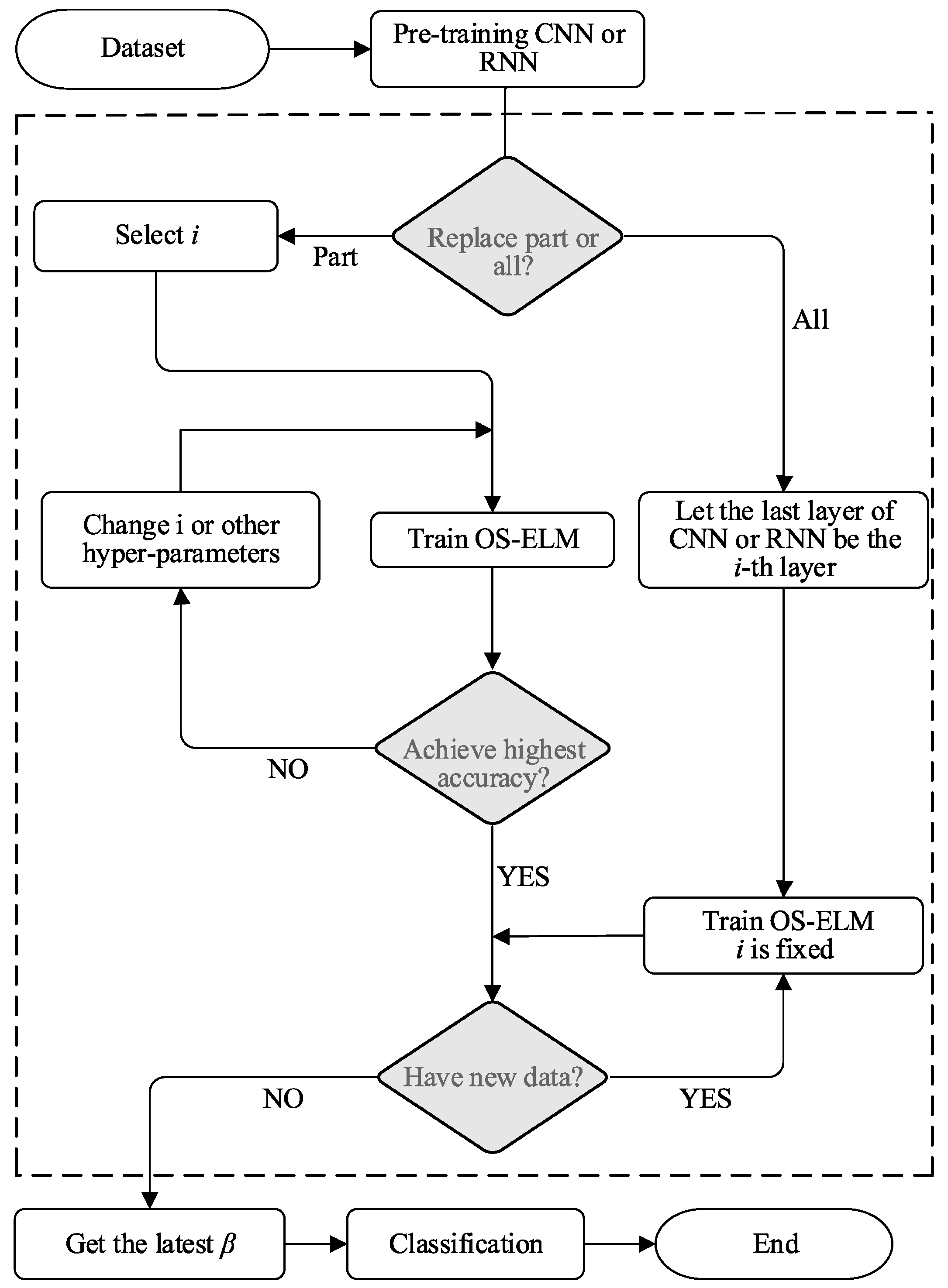
The fnnmOS-ELM online sequential learning process is simple. It is mainly divided into three parts, as shown in Figure 2.

The first involves obtaining pre-trained CNNs and RNNs. The second involves online sequential learning. Here, the network structure is divided into a “Part” and an “All” branch, where the “Part” branch is used to replace some or all of the network layers in the pre-training network classifier with the OS-ELM, and adjust the network structure and hyper-parameters based on classification accuracy; the “All” branch uses fnnmOS-ELM as the optimiser, connecting the OS-ELM to the CNNs and RNNs network layers, with the $i$-th network layer being the last. If new data arrives, the value of the output weight $\beta$ will be updated. If the data of the online sequential learning has been completely learned, the process enters the third part, whereby the feature is extracted using the network before the $i$-th layer, and after the $i$-th layer, the OS-ELM can process fast classification. The whole training process is relatively simple, and the network structure can be flexibly adjusted.

Algorithm 1 shows the hyper-parameters involved in the fnnmOS-ELM online learning process, as well as the updates of the output weight $\beta$. Some of the hyper-parameters will be discussed and studied in detail in Section 4.

Algorithm 1 Online sequential learning

1.  Preparation: (1) Pre-training model: (2) Truncate the ${\mathit{N}\mathit{e}\mathit{t}}_n$ output at the $i$-th layer and use it as input data for the model; 2.  Online learning: Input: the number of hidden nodes $\mathit{S}$, output data of the $i$-th layer, batch size $\mathit{D}$, and epochs are calculated from the data and $\mathit{D}$. Ouput: output weights $\beta$ of the fnnmOS-ELM model. 1.  Randomly select $W_i$ and $b_i$; 2.  Clculate: for $k=0$ to epoch $$\begin{array}{c}{P}_{k+1}=P_k-P_k{H}_{k+1}^T{\left(I+H_{k+1}{P}_k{H}_{k+1}^T\right)}^{-1}{H}_{k+1}{P}_k\\ {\beta }^{\left(k+1\right)}={\beta }^{\left(k\right)}+P_{k+1}{H}_{k+1}^T\left(T_{k+1}-H_{k+1}{\beta }^{\left(k\right)}\right)\end{array};$$ 3.  Get $\beta ={\beta }^{\left(k+1\right)}$; 4.  Combine the traditional neural networks before the $i$-th layer with the trained online learning model into the fnnmOS-ELM model; 5.  Adjust hyper-parameters: depending on the accuracy or the error of the classification on the test datasets. The hyper-parameters include three parts: $S$, $D$, and $i$; 6.  Return 1.

4. Experimental Design and Result Analysis

4.1. Dataset

In previous studies, OS-ELM was mostly used in datasets with small categories and data volume, such as DNA and the Image Segmentation dataset [40]. In this study, as listed in

Table 1. Datasets used in this paper.

Dataset	Classes	Training Data	Testing Data
Iris	3	90	60
IMDb	2	25,000	25,000
CIFAR-10	10	50,000	10,000
CIFAR-100	100	50,000	10,000

, we chose the Iris [41], IMDb [42], CIFAR-10, and CIFAR-100 [43] datasets to verify the performance of the fnnmOS-ELM. These choices were made considering the following aspects:

(1)

The Iris dataset is a commonly used classification dataset, which is often used for multiple variable analysis and testing the performance of linear classifiers. It is known that SVM and LR algorithms perform well in linear segmentation. Especially, the SVM made a breakthrough in the fields of binary and generalized linear classification [44]. Thus, we want to compare the performance of the fnnmOS-ELM on linear classification datasets.

(2)

IMDb is a dataset of 1000 popular movies from the last 10 years. It is often used in the field of natural language processing for short text sentiment analysis. LSTM [45], RNN, and other algorithms have shown good performance on this problem, so we want to test the performance of the fnnmOS-ELM on the same dataset.

(3)

CIFAR-10 and CIFAR-100 datasets have become two of the most popular datasets in recent years. They are basic datasets for image recognition. Using these datasets is beneficial to verify the performance of the fnnmOS-ELM in multi-classification and deep learning.

4.2. OS-ELM Mixed with Simple Neural Networks

In this study, we compare the performance of six methods on the Iris dataset, i.e., SVM, LR, Decision Tree, and KNN belong to four non-neural network algorithms, and the Simple Neural Network (Simple NN). The fnnmOS-ELM belongs to two algorithms with neural network structures. As shown in Figure 3b, the pre-training network used in the fnnmOS-ELM, including an input layer, two full connection layers, and two activation layers (ReLU function), were used [46].

As shown in

Table 2. Training time and parameters on the Iris dataset.

Dataset	Method		Training Time (s)	Trainable Parameters
Iris	SVM		<0.1	-
	LR		<0.1	-
	Decision Tree		<0.1	-
	KNN		<0.1	-
	Simple NN		16.7213	131
	fnnmOS-ELM	i = 3	0.5004	15
		i = 4	0.5084	15

, the four non-neural network structure algorithms have intrinsically short training time and small training parameter size. In this regard, Simple NN and fnnmOS-ELM do not have these advantages. The accuracy of the pre-training network Simple NN on the test data is 0.9533 ($\pm 0.02$). Then, the trained neural network parameters of the Simple NN and fnnmOS-ELM are frozen in the third ($i=3)$ and fourth ($i=4)$ layers of the network. As shown in Figure 3c, we access OS-ELM, where $Y$ is the output of activation1 after batch acquisition, $W$ is the random weight, and $\beta$ is the output weight to be trained. The batch size is set to 10 and the hidden nodes are set to 5. After 7-epoch training, the accuracy of Simple NN and fnnmOS-ELM increase to 0.9800 ($\pm 0.02$) and 0.9730 ($\pm 0.025$), respectively, as shown in Figure 3a. The Simple NN exceeds the accuracy of the fnnmOS-ELM on the same dataset, reducing the time for training and classification from 16 s to 0.5 s, while reducing the training parameter size by 8 times. It is worth remarking that we consider the time and parameter size required for training for a batch of new data in this study. The feature extraction layer parameters of the fnnmOS-ELM have been pre-trained and no further training is needed for the new data.

4.3. OS-ELM Mixed with RNN

On the IMDb dataset, we compare three commonly used algorithms without network structure, namely LR, Multinomial NB, as well as SDG, and three algorithms with network structure, i.e., LSTM, RNN, as well as fnnmOS-ELM. The comparison results are shown in

Table 3. Training time and parameters on the IMDb dataset.

Dataset	Method		Training Time (s)	Trainable Parameters
IMDb	TF-IDF	LR	<0.1	-
		Multinominal	<0.1	-
		NB
		SGD	<0.1	-
	LSTM		1178	438,045
	RNN		16.72	126,993
	fnnmOS-ELM	i = 4	1.15	10

. For enhancing the contrast effect of the fnnmOS-ELM and improving the accuracy, we introduce the TF-IDF statistical method [47] to the three algorithms without network structure after processing the data using the embedded layer [48]. The first three algorithms have advantages in training time and trainable parameters. After 20-epoch training, the accuracy of the pre-trained RNN (Figure 4b) reaches 0.8254, which is worse than LR, Multinomial NB, SGD, and LSTM. Then, we access the OS-ELM after the RNN layer (i = 4, Figure 4c), the hidden nodes were set to 10, the batch size was set to 100, and the training epoch was set to 40. From Figure 4a, it can be seen that the accuracy reaches 0.9925 (±0.005), which surpasses other algorithms tested on the same dataset, and the result enters the top 3 in the Kaggle leaderboard. Compared with the pre-trained RNN, the training time is reduced from 16.72 s to 1.15 s, and the trainable parameter size in the classifier is reduced to 10.

4.4. OS-ELM Mixed with CNN

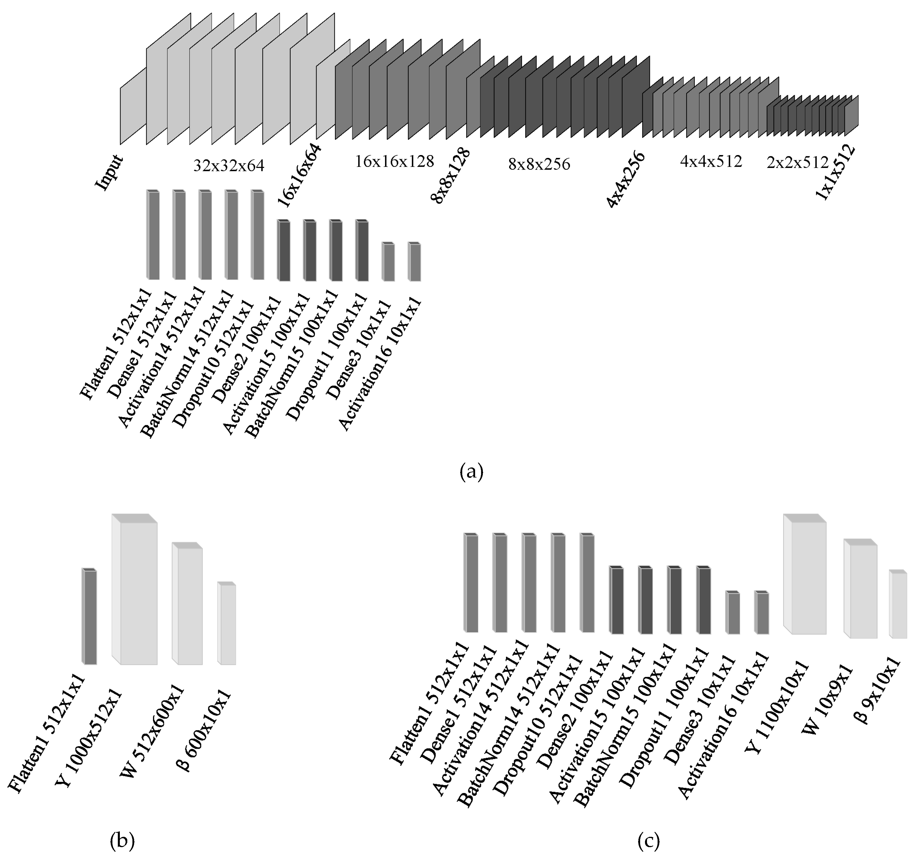
We now compare the performance of ResNet-110 [49], ELU [50], RCNN [51], VGG16 [52], ELM-LRF, CNN-ELM, and fnnmOS-ELM on the CIFAR-10 dataset. In ELM-LRF, we set the size of receptive field to 4 × 4, and the highest accuracy that can be achieved is lower than 85.3, and the result is unstable. The VGG16 used for feature extraction is shown in Figure 5a, and after making some minor changes to the VGG16 network, the highest accuracy achieved on the CIFAR-10 dataset is 93.01 ($\pm 0.3$, epoch = 40). CNN-ELM uses the feature maps of VGG16 as feature extractor and ELM as classifier. Its highest accuracy is less than 90.73, and the result is also unstable. With $i=55$, we access the fnnmOS-ELM (see Figure 5b) and set the hidden nodes of the network as 600. The training batch size and epochs are set to 1000 and 20, respectively. The maximum test accuracy of 0.9397, which exceeds that of the other methods or models (

Table 4. Trainable parameters and test accuracy of several methods on the CIFAR-10 and CIFAR-100 datasets.

Dataset	Method		Trainable Parameters	Test Accuracy (%)
CIFAR-10	ResNet-100		1.7 M	93.57
	ELU		>1 M	93.45
	RCNN		0.67 M	92.91
	VGG16		15 M	93.01 ($\pm$0.3)
	ELM-LRF		>10,000	<85.30
	CNN(VGG16)-ELM		>10,000	<90.73
	fnnmOS-ELM	i = 55	6000	93.97 ($\pm 0.1$)
		i = 65	90	93.80 ($\pm$0.1)
CIFAR-100	ELU		>1 M	75.72
	RCNN		1.87 M	68.25
	NIN+APL		0.67 M	69.17
	VGG16		15 M	69.73 ($\pm$0.59)
	ELM-LRF		0.1 M	<60.31
	CNN(VGG16)-ELM		0.1 M	<67.77
	fnnmOS-ELM	i = 55	85,000	70.64 ($\pm 0.1)$
		i = 65	7000	70.67 $\left(\pm 0.1\right)$

), has also entered the top 7 on Kaggle. Using the OS-ELM instead of full connection layers, not only improves the accuracy compared to the VGG16 network, but also reduces the parameters of new training data from 15M to 6K. The training time elapsed to achieve the highest accuracy is only approximately 1.55 s (CPU), which is much shorter than that of the most other methods (except ELM-LRF) that were tested on the same dataset. To verify the optimization effect of the fnnmOS-ELM on CNNs, the former is used as the optimiser of VGG16 classification, as in Figure 5c. Although we used only nine hidden nodes, the maximum accuracy is raised from 0.9301 to 0.9380, exceeding that of other algorithms tested on the same dataset.

On more complex CIFAR-100 dataset, we compare the performances of ELU, RCNN, NIN-APL [53], VGG16, ELM-LRF, and CNN-ELM with fnnmOS-ELM (using the VGG16 as a pre-training network). The structure of the fnnmOS-ELM network is the same as in Figure 5. After training 80 epochs, the highest accuracy of the VGG16 is 69.73 ($\pm 0.59$). It is lower than that of ELU and higher than that of RCNN and NIN-APL with much larger training parameters (Table 4). With $i = 55$, using OS-ELM as the classifier, we set the batch size to 1000 and epoch to 20, consisting of 850 hidden nodes, the accuracy of the test data is 0.7064, which is second only to ELU’s highest accuracy. When $i = 65$, we set hidden the nodes to 70, the batch size to 1000, and the epoch to 20, in order to optimize the classification accuracy of the VGG16. These settings improve the maximum accuracy from 69.73 to 70.67 (entering the top 3 on Kaggle). The accuracy of the fnnmOS-ELM on the test data exceeds that of the RNN, RCNN, and NIN-APL, at the same time, the highest accuracy of ELM-LRF (the receptive field size = 6 × 6) and CNN-ELM reached 60.31 and 67.77, respectively, which is not as good as our method. Although the accuracy of fnnmOS-ELM is lower than the highest accuracy of the ELU, it has much smaller trainable parameters than other models and the training time is less than 10 s (CPU).

4.5. Hyper-Parameters on CIFAR-10 Dataset

On the CIFAR-10 dataset, we examine the influence of hyper-parameters on the training effect in detail, and the performance of the fnnmOS-ELM model on the classification problems mentioned above did not achieve the best performance. If the hyper-parameters can be adjusted to a more appropriate state, the classification accuracy will be higher.

4.5.1. Impact of Batch Size D on Performance

On the CIFAR-10 dataset, we examine the influence of hyper-parameters on the training effect in detail, and the performance of the fnnmOS-ELM model on the classification problems mentioned above did not achieve the best performance. If the hyper-parameters can be adjusted to a more appropriate state, the classification accuracy will be higher.

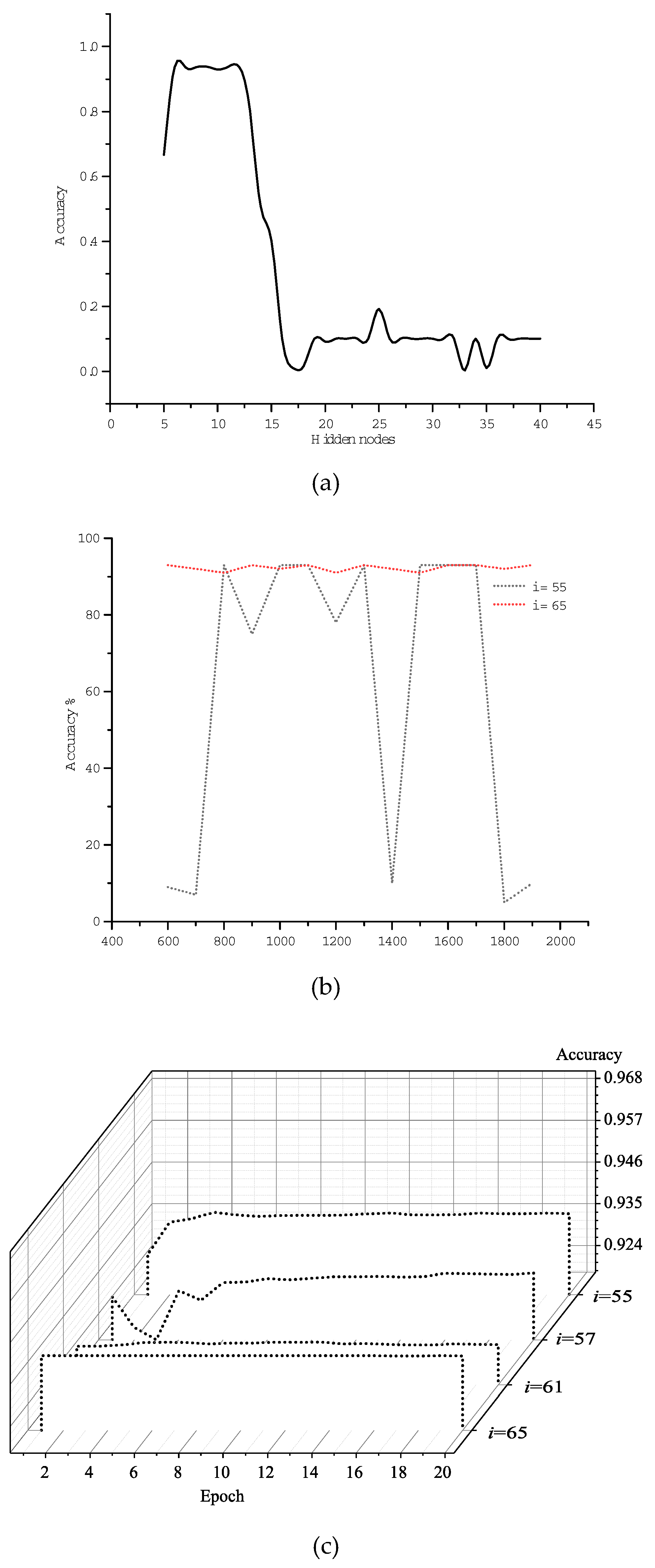
It is found that the batch size has a greater impact on the performance of fnnmOS-ELM. The fnnmOS-ELM uses the online learning method and learns data chunk-by-chunk. For traditional networks with gradient descent training, using a larger batch size will readily lead to the decline of the generalization performance, due to sharp minima. On the other hand, using a smaller batch size will lead to inherent noise, which will affect the speed of gradient variation [54]. Although the training process of the fnnmOS-ELM does not update the parameters by gradient descent, the batch size has also a great influence on the test accuracy. In Equations. (2) and (5), when the batch size ($D$) affects the dimension of $Y_{i0}$, it also affects the dimension of the $H_0$ matrix. As shown in Figure 6a, when $i = 55$, the fnnmOS-ELM replaces the fully connected layers in the network and the batch size has a large impact on the test accuracy. When $i = 65$, the fnnmOS-ELM is used as the optimiser of the original VGG16 network and the batch size has a small impact on the classification effect on the test accuracy. Therefore, when using the fnnmOS-ELM as an optimiser, a good performance can be achieved without repeatedly adjusting the batch size; when using the OS-ELM as a network classifier, it is beneficial to adjust the batch size to a suitable value.

4.5.2. Influence of i on Performance

After pre-training, it is necessary to decide from which layer $i$ of the network structure to access the fnnmOS-ELM. Generally, we consider the process of feature extraction of the pre-trained network and the classification performance of the mixed structure, replacing a part or all of the full connection layers, or simply optimizing the original network. In Figure 6b, we set $i = 65$ (hidden nodes = 9, batch size = 1000) and $i = 61$ (hidden nodes = 29, batch size = 1000). Compared with CNNs and RNNs, the fnnmOS-ELM shows a good classification performance on the test data at the beginning of the training, after which the performance remains stable. When $i = 57$ (hidden nodes = 100, batch size = 1000) and $i = 55$ (hidden nodes = 600, batch size = 1000), the initial performance fluctuates greatly. With increasing training epochs, the stability and accuracy are gradually improved.

If the value of $i$ is small, the training parameters of online learning will be reduced, but more epochs are required in training. If the value of $i$ is large, the training parameters will increase, but, at the same time, the performance of the network will tend to stabilise faster. This is because the classifier of RNNs and CNNs includes both the full connection layers and some additional layers that deal with special data. For example, Batch Norm layers can improve the stability [55] and Dropout layers can improve the generalization ability of networks [44]. When the OS-ELM is used to replace these layers, the performance will fluctuate.

4.5.3. Influence of Hidden Nodes S on Performance

The number of hidden nodes, the dimension of the output constitute $\beta$, and Equation (10) needs to be iterated through online learning to obtain the final $\beta$. On the one hand, the number of hidden nodes determines the size of $\beta$ and affects the number of trainable parameters and the training time. On the other hand, as shown in Figure 6c, they have a great impact on the classification performance of the fnnmOS-ELM. When different networks are used with the OS-ELM as pre-trained feature extraction networks, or different $i$ are used, the optimal number of hidden nodes for classification performance is different. If we assume that the dimensions of the output of the $i$-th network is $M$, with $0.5M\le$ hidden nodes $\le 1.5M$ the classification performance of the network is superior.

5. Conclusions and Future Work

The effectiveness of classification and optimization of fnnmOS-ELM has been numerically and experimentally investigated on Iris, IMDb, CIFAR-10 and CIFAR-100 datasets. Specifically, fnnmOS-ELM structure is established by mixing neural network and OS-ELM. Obtaining pre-trained CNNs and RNNs, online sequential learning and training OS-ELM are employed in fnnmOS-ELM training process. Furthermore, the hyper-parameters such as batch size, number of hidden nodes, and access layers of fnnmOS-ELM model on the training effect are investigated on CIFAR-10 dataset. Experimental results demonstrate that the fnnmOS-ELM combines the feature representation of CNNs and RNNs with the powerful classifier of OS-ELM. As an optimiser, the fnnmOS-ELM improves significantly in CNNs and RNNs classification performance. Compared with other algorithms or models, the fnnmOS-ELM exhibits shorter training time, fewer parameters, higher accuracy, and higher flexibility. Additionally, it is shown to be compatible with other models.

While the experiments focus primarily on the image classification tasks, the generality of fnnmOS-ELM showed in this paper provides a number of avenues for future work. In fact, in real life scenarios, fnnmOS-ELM can be applied to any model with neural network structure. For example, the combination of fnnmOS-ELM and transfer learning, which can be used to deal with more challenging video classification tasks. In addition, when we use fnnmOS-ELM for model-free RL reinforcement learning tasks, we have also achieved good results, which will be another exciting avenue for future work.

References

1. Krizhevsky, A.; Sutskever, I.; Hinton, G.E. Imagenet classification with deep convolutional neural networks. Commun. ACM 2017, 60, 84–90. [Google Scholar] [CrossRef]
2. Zeiler, M.D.; Fergus, R. Visualizing and understanding convolutional networks. In Proceedings of the European Conference on Computer Vision (ECCV), Zurich, Switzerland, 6–12 September 2014; pp. 818–833. [Google Scholar]
3. Zheng, S.; Jayasumana, S.; Romera-Paredes, B.; Vineet, V.; Su, Z.; Du, D.; Huang, C.; Torr, P.H.S. Conditional randomfields as recurrent neural networks. In Proceedings of the IEEE International Conference on Computer Vision (ICCV), Santiago, Chile, 7–13 December 2015; pp. 1529–1537. [Google Scholar]
4. Sermanet, P.; Eigen, D.; Zhang, X.; Mathieu, M.; Fergus, R.; Lecun, Y. Overfeat: Integrated recognition, localization and detection using convolutional networks. In Proceedings of the International Conference on Learning Representations, Banff, AB, Canada, 14–16 April 2014. [Google Scholar]
5. Taigman, Y.; Yang, M.; Ranzato, M.; Wolf, L. Deepface: Closing the gap to human level performance in face verification. In Proceedings of the IEEE Conference on Computer Vision and Pattern Recognition (CVPR), Columbus, OH, USA, 23–28 June 2014; pp. 1701–1708. [Google Scholar]
6. Jozefowicz, R.; Zaremba, W.; Sutskever, I. An empirical exploration of recurrent network architectures. In Proceedings of the 32nd International Conference on Machine Learning, Lille, France, 6–11 July 2015; pp. 2342–2350. [Google Scholar]
7. Hinton, G.; Deng, L.; Yu, D.; Dahl, G.E.; Mohamed, A.-r.; Jaitly, N.; Senior, A.; Vanhoucke, V.; Nguyen, P.; Sainath, T.; et al. Deep neural networks for acoustic modeling in speech recognition. IEEE Signal Process. Mag. 2012, 29, 82–97. [Google Scholar] [CrossRef]
8. LeCun, Y.; Bottou, L.; Orr, G.B.; Müller, K.-R. Efficient backprop. In Neural Networks: Tricks of the Trade; Lecture Notes in Computer Science; Montavon, G., Orr, G., Müller, K.R., Eds.; Springer: Berlin/Heidelberg, Germany, 2012; Volume 1524, pp. 9–50. [Google Scholar]
9. Svozil, D.; Kvasnicka, V.; Pospichal, J. Introduction to multi-layer feed-forward neural networks. Chemom. Intell. Lab. Syst. 1997, 39, 43–62. [Google Scholar] [CrossRef]
10. Huang, G.-B.; Zhu, Q.-Y.; Siew, C.-K. Extreme Learning Machine: A New Learning Scheme of Feedforward Neural Networks. In Proceedings of the 2004 IEEE International Joint Conference on Neural Networks, Budapest, Hungary, 25–29 July 2004; IEEE: Budapest, Hungary, 2004; pp. 985–990. [Google Scholar]
11. Huang, G.-B.; Siew, C.K. Extreme learning machine: RBF network case. In Proceedings of the 8th Control, Automation, Robotics and Vision Conference (ICARCV), Kunming, China, 6–9 December 2004; pp. 1029–1036. [Google Scholar]
12. Huang, G.-B.; Zhu, Q.-Y.; Mao, K.; Siew, C.K.; Saratchandran, P.; Sundararajan, N. Can threshold networks be trained directly? IEEE Trans. Circuits Syst. II Express Br. 2006, 53, 187–191. [Google Scholar] [CrossRef]
13. Huang, G.-B.; Zhu, Q.-Y.; Siew, C.K. Extreme learning machine: Theory and applications. Neurocomputing 2006, 70, 489–501. [Google Scholar] [CrossRef]
14. Huang, G.-B.; Chen, L.; Siew, C.K. Universal approximation using incremental constructive feedforward networks with random hidden nodes. IEEE Trans. Neural Netw. 2006, 17, 879–892. [Google Scholar] [CrossRef] [PubMed]
15. Liang, N.-Y.; Huang, G.-B.; Saratchandran, P.; Sundararajan, N. A fast and accurate online sequential learning algorithm for feedforward networks. IEEE Trans. Neural Netw. 2006, 17, 1411–1423. [Google Scholar] [CrossRef]
16. LeCun, Y.; Bengio, Y.; Hinton, G. Deep Learning. Nature 2015, 521, 436–444. [Google Scholar] [CrossRef]
17. Lecun, Y.; Bottou, L.; Bengio, Y.; Haffner, P. Gradient-based learning applied to document recognition. Proc. IEEE 1998, 86, 2278–2324. [Google Scholar] [CrossRef] [Green Version]
18. Xu, R.; Tao, Y.; Lu, Z.; Zhong, Y. Attention-Mechanism-Containing Neural Networks for High-Resolution Remote Sensing Image Classification. Remote Sens. 2018, 10, 1602. [Google Scholar] [CrossRef]
19. Siniscalchi, S.M.; Salerno, V.M. Adaptation to New Microphones Using Artificial Neural Networks with Trainable Activation Functions. IEEE Trans. Neural Netw. 2017, 28, 1959–1965. [Google Scholar] [CrossRef] [PubMed]
20. Chae, S.; Kwon, S.; Lee, D. Predicting Infectious Disease Using Deep Learning and Big Data. Int. J. Environ. Res. Public Health 2018, 15, 1596. [Google Scholar] [Green Version]
21. Ferrari, S.; Stengel, R.F. Smooth function approximation using neural networks. IEEE Trans. Neural Netw. 2005, 16, 24–38. [Google Scholar] [CrossRef] [PubMed]
22. Rumelhart, D.E.; Hinton, G.E.; Williams, R.J. Neurocomputing: Foundations of Research. In Learning Internal Representations by Error Propagation; MIT Press: Cambridge, MA, USA, 1988. [Google Scholar]
23. Xiang, C.; Ding, S.Q.; Lee, T.H. Geometrical interpretation and architecture selection of MLP. IEEE Trans. Neural Netw. 2005, 16, 84–96. [Google Scholar] [CrossRef] [PubMed]
24. Huang, G.-B.; Chen, Y.Q.; Babri, H.A. Classification ability of single hidden layer feedforward neural networks. IEEE Trans. Neural Netw. 2000, 11, 799–801. [Google Scholar] [CrossRef] [PubMed] [Green Version]
25. Wang, N.; Er, M.J.; Han, M. Generalized single-hidden layer feedforward networks for regression problems. IEEE Trans. Neural Netw. 2015, 26, 1161–1176. [Google Scholar] [CrossRef] [PubMed]
26. Gopal, S.; Fischer, M.M. Learning in single hidden-layer feedforward network models: Backpropagation in a spatial interaction modeling context. Geogr. Anal. 2010, 28, 38–55. [Google Scholar] [CrossRef]
27. Ngia, L.S.H.; Sjoberg, J.; Viberg, M. Adaptive neural nets filter using a recursive Levenberg-Marquardt search direction. In Proceedings of the Conference Record of the Thirty-Second Asilomar Conference on Signals, Systems & Computers, Pacific Grove, CA, USA, 1–4 November 1998; pp. 697–701. [Google Scholar]
28. Caruana, R.; Lawrence, S.; Giles, L. Overfitting in neural nets: Backpropagation, conjugate gradient, and early stopping. In Proceedings of the 13th International Conference on Neural Information Processing Systems, Denver, CO, USA, 27 November–2 December 2000; pp. 381–387. [Google Scholar]
29. Huang, G.-B. Learning capability and storage capacity of two-hidden-layer feedforward networks. IEEE Trans. Neural Netw. 2003, 14, 274–281. [Google Scholar] [CrossRef]
30. Tamura, S.; Tateishi, M. Capabilities of a four-layered feedforward neural network: Four layers versus three. IEEE Trans. Neural Netw. 1997, 8, 251–255. [Google Scholar] [CrossRef]
31. Banerjee, K.S. Generalized inverse of matrices and its applications. Technometrics 1973, 15, 197. [Google Scholar] [CrossRef]
32. Bai, Z.; Huang, G.-B.; Wang, D.; Wang, H.; Westover, M.B. Sparse extreme learning machine for classification. IEEE Trans. Syst. Man Cybern. 2014, 44, 1858–1870. [Google Scholar] [CrossRef] [PubMed]
33. Yang, Y.; Wu, Q.M.J.; Wang, Y.; Zeeshan, K.M.; Lin, X.; Yuan, X. Data partition learning with multiple extreme learningmachines. IEEE Trans. Syst. Man Cybern. 2015, 45, 1463–1475. [Google Scholar]
34. Luo, J.; Vong, C.-M.; Wong, P.-K. Sparse Bayesian extreme learning machine for multi-classification. IEEE Trans. Neural Netw. 2014, 25, 836–843. [Google Scholar]
35. Huang, G.-B.; Zhou, H.; Ding, X.; Zhang, R. Extreme learning machine for regression and multiclass classification. IEEE Trans. Syst. Man Cybern. Part B Cybern. 2012, 42, 513–529. [Google Scholar] [CrossRef] [PubMed]
36. Liu, X.; Wang, L.; Huang, G.-B.; Zhang, J.; Yin, J. Multiple kernel extreme learning machine. Neurocomputing 2015, 149, 253–264. [Google Scholar] [CrossRef]
37. Huang, G.-B.; Bai, Z.; Kasun, L.L.C.; Vong, C.-M. Local receptive fields based extreme learning machine. IEEE Comput. Intell. Mag. 2015, 10, 18–29. [Google Scholar] [CrossRef]
38. Duan, M.; Li, K.; Yang, C.; Li, K. A hybrid deep learning CNN-ELM for age and gender classification. Neurocomputing 2018, 275, 448–461. [Google Scholar] [CrossRef]
39. Srivastava, N.; Hinton, G.E.; Krizhevsky, A.; Sutskever, I.; Salakhutdinov, R. Dropout: A simple way to prevent neural networks from overfitting. J. Mach. Learn. Res. 2014, 15, 1929–1958. [Google Scholar]
40. Blake, C.L. UCI Repository of Machine Learning Databases. Available online: http://archive.ics.uci.edu/ml/index.php (accessed on 25 June 2019).
41. Daugman, J. New methods in iris recognition. IEEE Trans. Syst. Man Cybern. Part B (Cybern.) 2007, 37, 1167–1175. [Google Scholar] [CrossRef]
42. Ahmed, A.; Batagelj, V.; Fu, X.; Hong, S.-H.; Merrick, D.; Mrvar, A. Visualisation and analysis of the internet movie database. In Proceedings of the 6th International Asia-Pacific Symposium on Visualization, Sydney, Australia, 5–7 February 2007; pp. 17–24. [Google Scholar]
43. Krizhevsky, A. Learning Multiple Layers of Features from Tiny Images; Tech. Rep. 001; Department of Computer Science, University of Toronto: Toronto, Canada, 2009. [Google Scholar]
44. Ben-Hur, A.; Horn, D.; Siegelmann, H.T.; Vapnik, V. A support vector method for clustering. In Proceedings of the 13th International Conference on Neural Information Processing Systems, Barcelona, Spain, 3–7 September 2000; pp. 367–373. [Google Scholar]
45. Shi, X.; Chen, Z.; Wang, H.; Yeung, D.Y.; Wong, W.K.; Woo, W. Convolutional LSTM network: A machine learning approach for precipitation nowcasting. In Advances in Neural Information Processing Systems; MIT Press Cambridg: Cambridge, MA, USA, 2015; pp. 802–810. [Google Scholar]
46. Glorot, X.; Bordes, A.; Bengio, Y. Deep sparse rectifier neural networks. In Proceedings of the 14th International Conference on Artificial Intelligence and Statistics, Ft. Lauderdale, FL, USA, 11–13 April 2011; pp. 315–323. [Google Scholar]
47. Salton, G.; Buckley, C. Term-weighting approaches in automatic text retrieval. Inf. Process. Manag. 1988, 24, 513–523. [Google Scholar] [CrossRef] [Green Version]
48. Tang, J.; Qu, M.; Wang, M.; Zhang, M.; Yan, J.; Mei, Q. Line: Large-scale information network embedding. In Proceedings of the 24th International Conference on World Wide Web, Florence, Italy, 18–22 May 2015; pp. 1067–1077. [Google Scholar]
49. He, K.; Zhang, X.; Ren, S.; Sun, J. Identity mappings in deep residual networks. In Proceedings of the European Conference on Computer Vision (ECCV), Amsterdam, The Netherlands, 11–14 October 2016; pp. 630–645. [Google Scholar]
50. Clevert, D.-A.; Unterthiner, T.; Hochreiter, S. Fast and accurate deep network learning by exponential linear units (ELUs). In Proceedings of the International Conference on Learning Representations (ICLR), San Juan, Puerto Rico, 2–4 May 2016; pp. 1–14. [Google Scholar]
51. Liang, M.; Hu, X. Recurrent convolutional neural network for object recognition. In Proceedings of the IEEE Conference on Computer Vision and Pattern Recognition (CVPR), Boston, MA, USA, 7–12 June 2015; pp. 3367–3375. [Google Scholar]
52. Simonyan, K.; Zisserman, A. Very deep convolutional networks for large-scale image recognition. arXiv 2014, arXiv:1409.1556. [Google Scholar]
53. Agostinelli, F.; Hoffman, M.D.; Sadowski, P.J.; Baldi, P. Learning activation functions to improve deep neural networks. arXiv 2014, arXiv:1412.6830. [Google Scholar]
54. Keskar, N.S.; Mudigere, D.; Nocedal, J.; Smelyanskiy, M.; Tang, P.T.P. On largebatch training for deep learning: Generalization gap and sharp minima. arXiv 2016, arXiv:1609.04836. [Google Scholar]
55. Ioffe, S.; Szegedy, C. Batch normalization: Accelerating deep network training by reducing internal covariate shift. In Proceedings of the 32nd International Conference on Machine Learning, Lile, France, 6–11 July 2015; pp. 448–456. [Google Scholar]
Figure 1. Network structures of a traditional neural network and fnnmOS-ELM (online sequential extreme learning machine) models. (a) The OS-ELM is used as a classifier in the original network. (b) The OS-ELM replaces part of the network layers of the classifier in the original network. (c) The fnnmOS-ELM is used as the optimiser of the original network.
Applsci 09 03772 g001
Figure 2. The training process.
Applsci 09 03772 g002
Figure 3. Comparison of six models on the Iris dataset. (a) Accuracy. (b) Structure adopted by Simple Network. (c) Structure of the Simple Network when i = 3.
Applsci 09 03772 g003
Figure 4. Performance of different methods and network structures. (a) Comparison of accuracy. (b) Network structure of the recurrent neural network (RNN) model. (c) With i = 4, the fnnmOS-ELM model uses the first four layers of the RNN as the feature extraction layers.
Applsci 09 03772 g004
Figure 5. The network structure of VGG16 and fnnmOS-ELM. (a) Modified VGG16 network structure used as the pre-training model, divided into two parts: feature ex- traction and classifier. The fnnmOS-ELM network structure on the CIFAR-10 dataset with (b) i = 55 and (c) i = 65.
Applsci 09 03772 g005
Figure 6. Experimental results of different hyper-parameters on CIFAR-10. (a) Effect of batch size on the accuracy of the CIFAR-10 test data at i = 65 and 55 and epoch = 8. (b) When i takes different values, the accuracy of the fnnmOS-ELM model on the test data varies with the value of epoch. (c) When i = 65, the accuracy varies with the number of hidden nodes.
Applsci 09 03772 g006