Featured Application
Obtain exact solutions for the design of shear deformable functionally graded beams; verify new structural models; code computer program for shear deformable frames.
Abstract
Shear deformable beams have been widely used in engineering applications. Based on the matrix structural analysis (MSA), this paper presents a method for the buckling and second-order solutions of shear deformable beams, which allows the use of one element per member for the exact solution. To develop the second-order MSA method, this paper develops the element stability stiffness matrix of axial-loaded Timoshenko beam–columns, which relates the element-end deformations (translation and rotation angle) and corresponding forces (shear force and bending moment). First, an equilibrium analysis of an axial-loaded Timoshenko beam–column is conducted, and the element flexural deformations and forces are solved exactly from the governing differential equation. The element stability stiffness matrix is derived with a focus on the element-end deformations and the corresponding forces. Then, a matrix structural analysis approach for the elastic buckling analysis of Timoshenko beam–columns is established and demonstrated using classical application examples. Discussions on the errors of a previous simplified expression of the stability stiffness matrix is presented by comparing with the derived exact expression. In addition, the asymptotic behavior of the stability stiffness matrix to the first-order stiffness matrix is noted.
1. Introduction
Although a number of computer programs such as Abaqus, OpenSees, Ansys, and MSC.Marc are readily available for the structural analysis of frames, approaches to obtain the exact solutions in closed form are helpful in many situations. The exact analytical or numerical solutions are useful for ready use by engineers and researchers, for understanding the basic structural concepts, and for computational efficiency, for example, conducting parametric analysis conveniently based on an exact solution. In addition, the exact solutions may be used for verifying new structural analysis methods.
Among the various structural analysis methods [1,2,3,4,5,6], the matrix structural analysis [7,8,9,10,11,12,13,14,15] is found to be an efficient method ideally suitable for obtaining the exact solutions and for convenient computer implementations. The matrix structural analysis approach is essentially a matrix form of the displacement (stiffness) method [16,17] in basic structural mechanics and has been widely used in the traditional analysis associated with the flexural deformations of beam–column elements. This approach analyzes each member as an element and focuses on the element-end deformations and forces. The element-end deformation–force relationship is governed by the element stiffness matrix, which can be assembled to be the structural stiffness matrix for analysis of the entire structure. Therefore, formulating the element stiffness matrix is essential for the matrix analysis approach.
In the matrix structural analysis of the solutions for the buckling and second-order effect, the second-order effect (i.e., geometric nonlinearity) of beam–columns can be considered by using the exact element stability stiffness matrix. This second-order matrix structural analysis considering geometric nonlinearity has been verified in many classical publications as well as new applications (e.g., [7,8,11,13,14,15,18]).
This paper undertakes the formulation of the element second-order stiffness matrix (or stability stiffness matrix) of axial-loaded Timoshenko beam–columns considering geometric nonlinearity and the application of the stiffness matrix for stability analyses. An equilibrium analysis of an axial-loaded Timoshenko beam–column is conducted, and the element flexural deformations (translation and rotation angle) and corresponding forces (shear force and bending moment) are analyzed. The element stability stiffness matrix is derived to show the relationship between the element-end flexural deformations and the corresponding forces. A matrix structural analysis approach for the elastic buckling analysis of Timoshenko beam–columns is then established, and classical application examples are further presented. The errors of a previous simplified expression of the stability stiffness matrix are discussed by comparison with the exact expression.
2. Traditional Matrix Structural Analysis (MSA)
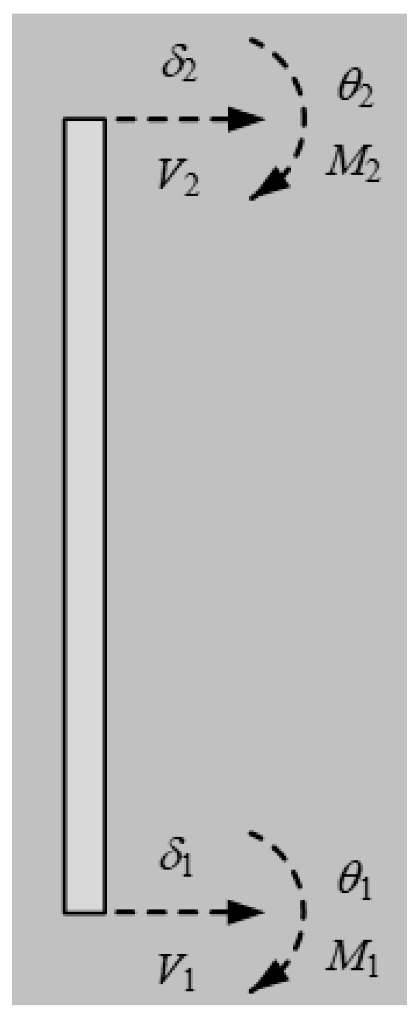
The traditional matrix structural analysis approach mainly focuses on the analysis of Euler–Bernoulli beam–columns. For first-order and second-order analysis (without and with considering the geometric nonlinearity), the element stiffness matrix of an Euler–Bernoulli beam–column element is formulated (e.g., [16,17]) as Equations (1) and (2), respectively, showing the relationship between the element-end translational deformations/rotation angles (δ1, θ1, δ2, θ2) and shear forces/bending moments (V1, M1, V2, M2) (see Figure 1). Based on the element stiffness matrix, structural analyses can be conveniently conducted, including the traditional first-order analysis for the element deformations and internal forces using Equation (1) (e.g., [16,17]), as well as elastic buckling and second-order stability analyses using Equation (2) (e.g., [13,14,15]).
where EI denotes the cross-sectional flexural rigidity; L denotes the element length; TEB, QEB, SEB, and CEB are element stability functions of factor λEB; λEB is an axial force factor for Euler–Bernoulli beam, defined as Equation (3); PE = π2EI/L2 is the Euler buckling axial force.

Figure 1.
An axial-loaded beam–column with element-end displacements and forces.
For the analysis of Timoshenko beam–columns, the cross-sectional shear deformations are considered, and the element stiffness matrix is a little more complex than that of Euler–Bernoulli beam–columns. The first-order element stiffness matrix (without considering geometric nonlinearity) has been widely known, as shown in Equation (4) [18,19]. However, for the second-order analysis (including the elastic buckling analysis), the exact solution of the element stiffness matrix considering geometric nonlinearity has not been derived. Ekhande et al. [18] provided a simplified form (Equation (5)) for this second-order element stiffness matrix (also denoted as stability stiffness matrix) of Timoshenko beam–columns, based on a modification of the second-order element stiffness matrix of Euler–Bernoulli beam–columns (Equation (2)). However, this simplified form uses modified element stability functions, which could have considerable errors for elements with large axial force. Thus, conducting (elastic buckling and second-order) analyses of axial-loaded Timoshenko beam–columns based on this simplified form could lead to incorrect results with large errors. Therefore, an exact element stiffness matrix for the axial-loaded Timoshenko beam–columns is required for the stability analysis of the Timoshenko beam–column system.
where φ is a dimensionless cross-sectional property of Timoshenko beams, which is defined based on the ratio of the flexural rigidity and the shear rigidity [6,18]. It is noted that this cross-sectional factor φ corresponds to the extent of the shear deformation effect in the Timoshenko beam–column.
3. Matrix Structural Analysis for Exact Solutions of Shear Deformable Beams
3.1. Relationship between Element-End Displacements and Forces
A shear deformable Timoshenko beam–column as shown in Figure 2 is analyzed. The beam–column has a length L, flexural rigidity EI, shear rigidity GA, and is subjected to an axial load P.

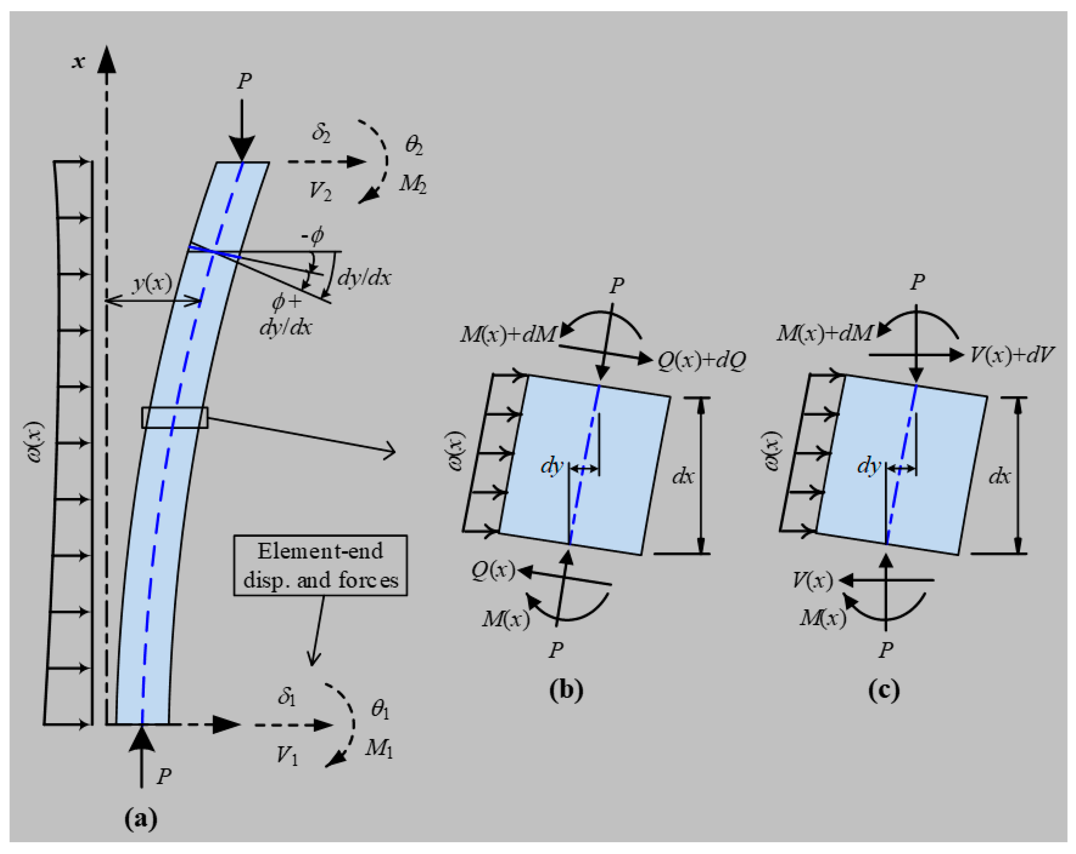
Figure 2.
Equilibrium analysis of axial-loaded Timoshenko beam–column: (a) analyzed element; (b) equilibrium of element short segment with shear force Q(x) normal to the deformed element axis; (c) element short segment with shear force V(x) normal to the undeformed element axis.
There are many classical researches on the equilibrium analysis of beam–columns considering the second-order effect. This paper focuses on the element-end displacements and forces based on the matrix approach. The derivations for the element-end displacements and forces of the beam–column in Figure 2 follow from the classical research, and they are presented in Appendix A. The small displacement assumption and the Timoshenko beam theory (TBT) are used in the analysis. The element deformation is solved exactly from the governing differential Equation (A8). Therefore, the use of one element per member for the exact solution could be allowed.
Based on the derivations, the element-end translational displacement/rotation angle and the corresponding shear force/bending moment of the beam–column can be expressed in matrix forms as (see Appendix A)
where ξ1, ξ2, ξ3, and ξ4 are combination factors for the element deformation; λ denotes an axial force factor for the Timoshenko beam, defined as Equation (9), in which a coefficient χ is defined as Equation (10) for the shear deformation effect. The axial compressive force can be expressed as Equation (11) based on Equation (9).
Combining Equations (10) and (11), the coefficient χ can be expressed as a function of the axial force factor λ and the dimensionless factor φ (Equation (12)). The axial compressive force P can then be expressed as Equation (13) based on Equation (11).
Combining Equations (7) and (8), the relationship between the element-end displacement vector (translations/rotation angles) and force vector (shear forces/bending moments) is formulated as
where [KTB,2nd] is defined as the element stability stiffness matrix for the relationship between the element-end displacement vector (translations/rotation angles) and force vector (shear forces/bending moments). Further, [KTB,2nd] can be derived to a simplified form as
3.2. Second-Order MSA for Exact Buckling Solutions of Shear Deformable Beams
Based on the element stability stiffness matrix, a matrix structural analysis approach for the exact elastic buckling analysis of Timoshenko beam–columns can be established. By considering all unrestrained member-end deformations, the structural stiffness matrix [K]s is formulated. Then, the MSA method can be applied for the elastic buckling analysis, by finding the minimum positive root Pcr of the axial load in a governing equation det [K]s = 0 [14,15].
4. Applications and Discussions
4.1. Elastic Buckling Analysis of Shear Deformable Columns
In this section, classical application examples of a Timoshenko column with typical element-end boundary conditions are presented, and the results are listed in Table 1.

Table 1.
Elastic buckling analysis of a Timoshenko column with typical boundary conditions.
For a pinned–pinned Timoshenko column (Case 1), the unrestrained element-end deformations are the element-end rotations. Therefore, the buckling state is corresponding to the condition that the determinant of the submatrix for the element-end rotations (second and fourth row/column of the element stiffness matrix [KTB], which is the structural stiffness matrix in this case) equals zero, and the buckling condition in this case can be solved as
For a fixed–free Timoshenko column (Case 2), the unrestrained element-end deformations are the translation and rotation at the free end. Therefore, the buckling state is corresponding to the condition that the determinant of the stiffness matrix at the free end (first two or last two row/column of the element stiffness matrix [KTB], which is the structural stiffness matrix in this case) equals zero, and the buckling condition in this case can be solved as
For a fixed–clamped Timoshenko column (Case 3), the only unrestrained element-end deformation is the translational displacement at the sliding clamped end. The relationship between this unrestrained translational displacement and the corresponding element-end shear force is defined by TTB. Therefore, the buckling state is corresponding to the condition that TTB = 0. Based on Figure 3 in Section 4.3, TTB decreases to 0 as λ increases to π. Therefore, the buckling condition in this case can be solved as
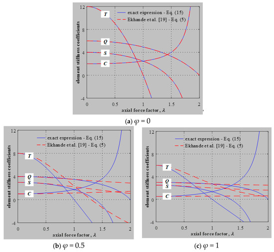
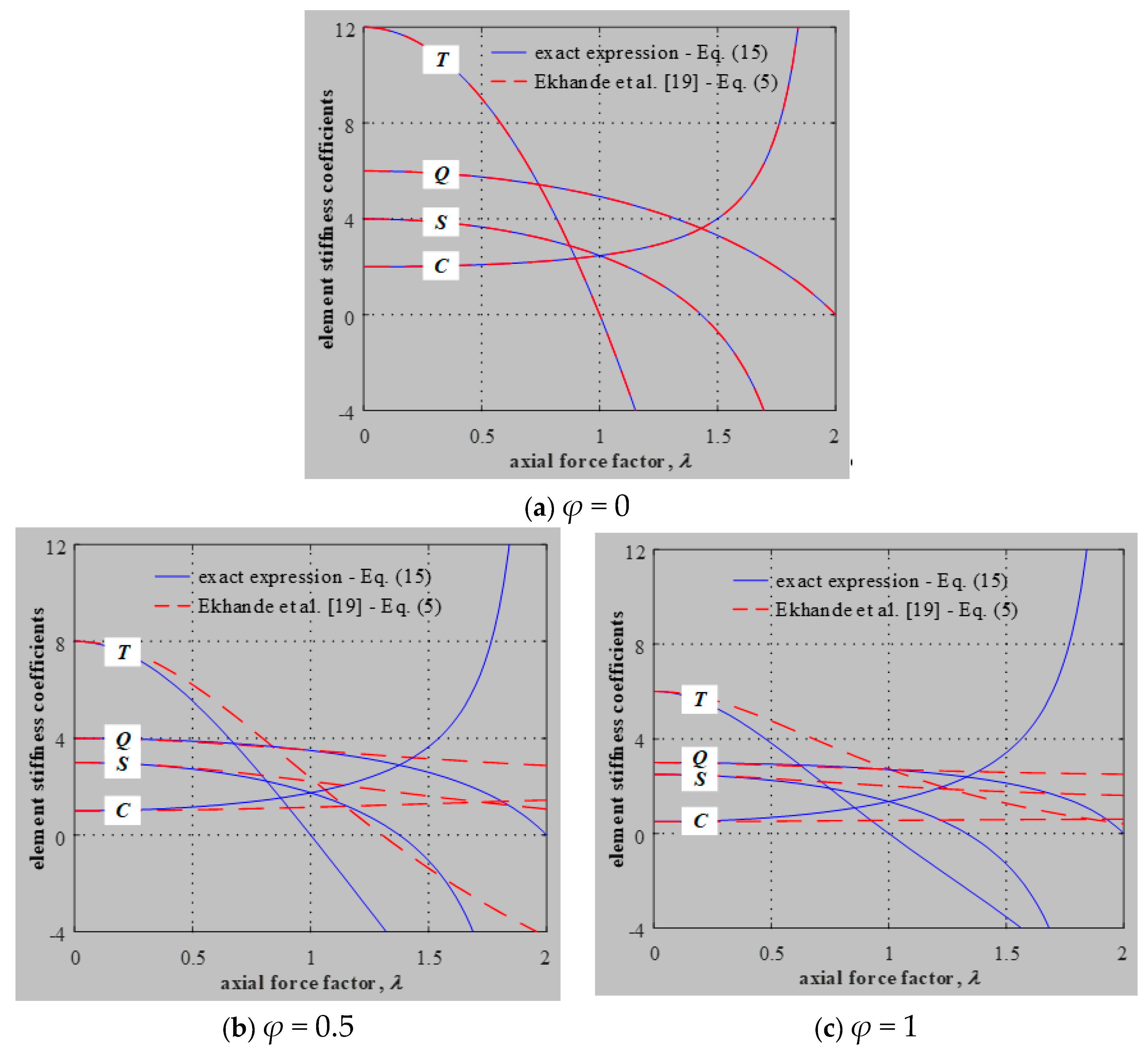
Figure 3.
Influence of axial force factor on element stability functions by Equation (15) (exact expression) and Equation (5) (simplified expression by Ekhande et al. [18]).
For a fixed–pinned Timoshenko column (Case 4), the only unrestrained element-end deformation is the rotation at the pinned end. The relationship between this unrestrained rotation and the corresponding element-end bending moment can be defined by STB. Therefore, the buckling state is corresponding to the condition that STB = 0. Based on Figure 3 in Section 4.3, STB decreases to 0 as λ increases to 1.43π (π/0.7). Therefore, the buckling condition in this case can be solved as
In addition, for a fixed–fixed Timoshenko column (case 5), the buckling state is corresponding to the condition that the denominator ϕTB in TTB, QTB, STB, and CTB equals zero [13]. Based on Equation (15), ϕTB decreases to 0 as λ increases to 2π. Therefore, the buckling condition in this case can be solved as
It is noted that this section gives the same results as those from classical analyses by Wang et al. [3], but the matrix analysis procedure is more simplified and systematic. Therefore, the derived Equation (15) for the stability stiffness matrix of an axial-loaded Timoshenko beam–column is verified.
4.2. Obtaining First-Order Stiffness Matrix
For the special condition of a Timoshenko beam with no axial load, the first-order Timoshenko beam element stiffness matrix (without considering geometric nonlinearity) (i.e., Equation (4)) can be derived from the stability stiffness matrix formulated in Equation (15). Considering the relationship in Equation (12), the element stability functions TTB, QTB, STB, and CTB in Equation (15) are functions of the axial force factor λ and the dimensionless factor φ. By taking the limit of Equation (15) as λ approaches zero (which corresponds to zero axial load), the element stiffness matrix of the Timoshenko beam without considering geometric nonlinearity can be derived to the same form as Equation (4). This finding also verifies the correctness of the derived stability stiffness matrix (Equation (15)) in the previous section.
4.3. Comparison with the Simplified Expression by Ekhande et al.
The element stability functions TTB, QTB, STB, and CTB are the basic properties for the element load-deformation responses. These stability functions correspond to the element-end shear force or bending moment for a unit element-end translation or rotation angle. The stability functions are transcendental functions of the axial force factor λ for given cross-sectional property factor φ. The different expressions of the element stability stiffness matrix in Equations (5) and (15) are essentially defined by the different expressions of the element stability functions. In the simplified expression (Equation (5)), the element stability functions are modified from the element stability functions TEB, QEB, SEB, and CEB of axial-loaded Euler–Bernoulli beam–columns, which are functions of the axial force factor λEB for Euler–Bernoulli beams. In addition, the relationship between the axial force factor λ and λEB (for Timoshenko and Euler–Bernoulli beams, respectively) can be derived based on Equations (9) and (12).
The element stability functions TEk, QEk, SEk, and CEk by Ekhande et al. [18] is a simplified expression that is not derived exactly, so it could result in errors in some situations comparing with the exact stiffness matrix (Equation (15)). Figure 3 shows the comparison of the exact (Equation (15)) and simplified (Equation (5)) expressions of the element stability functions as the axial force factor λ varies. In Figure 3a–c, the cross-sectional property factor φ is fixed to typical given values of 0, 0.5, and 1, respectively, which corresponds to an increase in the shear deformation effect.
Figure 3 shows that the element stability functions TTB, QTB, and STB decreases (while CTB increases) with the increasing axial force factor λ. As shown in Figure 3a, for a cross-sectional property factor of φ = 0 (which corresponds to zero shear deformation effect, i.e., the situation of Euler–Bernoulli beam–columns), the element stability functions by Ekhande et al. [18] (Equation (5)) give the same result as the derived exact stiffness matrix (Equation (15)). In addition, for an axial force factor of λ = 0, Figure 3b,c also shows that the two formulations give the same result. This is because the simplified form (Equation (5)) for the element stiffness matrix by Ekhande et al. [18] is defined based on these conditions. However, when the shear deformation effect is considered, the simplified form by Ekhande et al. [18] varies considerably with the derived exact stiffness matrix (Equation (15)), and the variation may be significant for a relatively large axial force factor. Therefore, for the condition of a relatively large axial force factor, the exact element stability stiffness matrix of Timoshenko beam–columns derived in this paper is recommended to be used because the simplified form by Ekhande et al. [18] could lead to large errors.
As an example, consider the elastic buckling problem of a fixed-clamped Timoshenko column. The exact buckling load is solved by Case 3 in Section 4.1. Next, the stiffness matrix in Equation (5) by Ekhande et al. [18] is used to obtain the buckling load. Then, the buckling state is corresponding to the condition that TEk = 0, and the buckling load in this case can be solved as follows
By comparing Equations (18) and (22), it is found that the elastic buckling load solved from Equation (5) is considerably larger than the exact elastic buckling load in this fixed-clamped case, and their difference is derived as . As the cross-sectional property factor φ increases (i.e., shear deformation effect increases), the error of the elastic buckling load solved from Equation (5) also increases. For the case of φ = 0.5 and 1, the error to the exact solution is 41.1% and 82.2%, respectively.
5. Summary and Conclusions
This paper presents the derivation, application, and discussions of the stability stiffness matrix of axial-loaded Timoshenko beam–columns. The main conclusions are summarized as follows:
- Equilibrium analysis of an axial-loaded Timoshenko beam–column is conducted based on the equilibrium conditions of shear force and bending moment of an element short segment, and a fourth-order governing differential equation is established. The solution of the differential equation can be used to analyze the element deformations and forces. Then, the element stability stiffness matrix is formulated, showing the relationship between the element-end flexural deformations and the corresponding forces.
- Based on the element stability stiffness matrix, a matrix structural analysis approach for the elastic buckling analysis of axial-loaded Timoshenko beam–columns is established. First, the structural stiffness matrix is assembled from the element stiffness matrix to show global structural responses. The eigenproblem for an elastic buckling analysis is then solved by setting the determinant of the structural stiffness matrix to zero. The established matrix analysis approach is demonstrated using classical elastic buckling analysis examples of the Timoshenko column with typical element-end boundary conditions.
- The simplified form for the element stability stiffness matrix of Timoshenko beam–columns by Ekhande et al. [18] could lead to large errors because it is defined considering the conditions that it gives the same result as the exact solution for zero shear deformation effect or zero axial force effect. However, for the condition of a relatively large axial force factor, the exact element stability stiffness matrix derived in this paper should be used.
Author Contributions
All three authors have contributed to the idea discussion, equation derivation, and manuscript drafting of this paper.
Funding
This research has received no external funding.
Conflicts of Interest
The authors declare no conflicts of interest.
Appendix A. Equilibrium Analysis of Shear Deformable Timoshenko Beam–Column
To establish the equilibrium conditions, a short segment of the element with length dx is analyzed, as depicted in Figure 2b,c, where the shear force is shown using Q(x) (which is defined to be normal to deformed element axis) and V(x) (which is defined to be normal to the undeformed element axis), respectively. The different compositions of shear force in Figure 2b,c give the relationship between Q(x) and V(x):
where x denotes the longitudinal coordinate of the element; y denotes the translational displacement.
The equilibrium of bending moment (using Figure 2b) and shear force (using Figure 2c) give Equations (A2) and (A3), respectively.
where M denotes the bending moment; P denotes the axial compressive force; ώ(x) denotes distributed lateral load.
According to the Timoshenko beam theory, the bending moment M and the shear force Q are given by
where ϕ denotes the rotation angle in the Timoshenko beam (defined as positive in the anticlockwise direction); GA denotes the cross-sectional shear rigidity; ks denotes the shear correction coefficient to account for the difference in the constant state of shear stress in the Timoshenko beam theory and the parabolic variation of the actual shear stress through the depth of the cross-section [6,19].
By substituting Equations (A2) and (A4) into Equation (A3), a relationship between ϕ and y is derived as
By substituting Equation (A5) into Equation (A3), a governing equation is derived as
Combining Equations (A6) and (A7), a fourth-order governing differential equation is derived as Equation (A8) for null distributed translational load (ώ = 0).
where λ denotes an axial force factor for the Timoshenko beam, defined as Equation (A9), in which a coefficient χ is defined as Equation (A10) for the shear deformation effect.
The solution of y(x) in the governing differential Equation (A8) is given by a linear combination of trigonometric functions and the linear polynomial function (Equation (A11)), using the deformation combination factors ξ1, ξ2, ξ3, and ξ4. The rotation angle ϕ can then be solved as Equation (A12) based on Equation (A7).
The element bending moment [M(x)] and shear force [Q(x) and V(x)] can then be formulated as Equations (A13), (A14), and (A15) based on Equations (A4), (A5), and (A1), respectively.
For a matrix structural analysis, the element-end displacements and corresponding forces are discussed in matrix forms. Based on Equations (A11) and (A12), the element-end displacement vector (translations/rotation angles) is formulated in a matrix-form relationship with the four deformation combination factors, as shown in Equation (A16).
Based on Equations (A13) and (A15), the element-end force vector (shear forces/bending moments, defined in Figure 2a) is also formulated in a matrix form, as shown in Equation (A17). It is noted that the direction of the element-end shear forces are defined based on the undeformed element axis, and thus the global structural analysis could be conducted.
References
- Galambos, T.V.; Surovek, A.E. Structural Stability of Steel: Concepts and Applications for Structural Engineers; John Wiley & Sons: Hoboken, NJ, USA, 2008. [Google Scholar]
- Trahair, N.S.; Bradford, M.A.; Nethercot, D.A.; Gardner, L. The Behaviour and Design of Steel Structures to EC3, 4th ed.; Taylor & Francis: Abingdon, UK, 2008. [Google Scholar]
- Wang, C.M.; Wang, C.Y.; Reddy, J.N. Exact Solutions for Buckling of Structural Members; CRC Press: Boca Raton, FL, USA, 2004. [Google Scholar]
- Chen, J. Stability of Steel Structures: Theory and Design, 5th ed.; Science Press: Beijing, China, 2011. (In Chinese) [Google Scholar]
- Chen, W.F.; Atsuta, T. In-plane behavior and design. In Theory of Beam-Columns; J. Ross Publishing: Plantation, FL, USA, 2007; Volume 1. [Google Scholar]
- Timoshenko, S.P.; Gere, J.M. Theory of Elastic Stability; McGraw Hill: New York, NY, USA, 1961. [Google Scholar]
- McGuire, W.; Gallagher, R.H.; Ziemian, R.D. Matrix Structural Analysis, 2nd ed.; John Wiley & Sons: Hoboken, NJ, USA, 2014. [Google Scholar]
- Przemieniecki, J.S. Theory of Matrix Structural Analysis; McGraw-Hill: New York, NY, USA, 1968. [Google Scholar]
- Beaufait, F.W.; Rowan, W.H., Jr.; Hoadley, P.G.; Hackett, R.M. Computer Methods of Structural Analysis; Prentice-Hall: Upper Saddle River, NJ, USA, 1970. [Google Scholar]
- Yang, Y.B.; McGuire, W. Stiffness matrix for geometric nonlinear analysis. J. Struct. Eng. 1986, 112, 853–877. [Google Scholar] [CrossRef]
- Munoz, H.R. Elastic Second-Order Computer Analysis of Beam–Columns and Frames. Master’s Thesis, University of Texas at Austin, Austin, TX, USA, 1991. [Google Scholar]
- Colorado-Urrea, G.J.; Aristizabal-Ochoa, J.D. Second-order stiffness matrix and load vector of an imperfect beam–column with generalized end conditions on a two-parameter elastic foundation. Eng. Struct. 2014, 70, 260–270. [Google Scholar] [CrossRef]
- Yuan, S. Programming Structural Mechanics, 2nd ed.; Higher Education Press: Beijing, China, 2008. (In Chinese) [Google Scholar]
- Pan, W.H.; Eatherton, M.R.; Tao, M.X.; Yang, Y.; Nie, X. Design of single-level guyed towers considering interrelationship between bracing strength and rigidity requirements. J. Struct. Eng. 2017, 143, 04017128. [Google Scholar] [CrossRef]
- Pan, W.H.; Eatherton, M.R.; Nie, X.; Fan, J.S. Stability and adequate bracing design of pre-tensioned cable braced inverted-Y-shaped Ferris wheel support system using matrix structural second-order analysis approach. J. Struct. Eng. 2018, 144, 04018194. [Google Scholar] [CrossRef]
- Hibbeler, R.C. Structural Analysis, 8th ed.; Pearson: London, UK, 2009. [Google Scholar]
- Long, Y.Q.; Bao, S.H.; Kuang, W.Q.; Yuan, S. Structural Mechanics, 2nd ed.; Higher Education Press: Beijing, China, 2006. (In Chinese) [Google Scholar]
- Ekhande, S.G.; Selvappalam, M.; Madugula, M.K.S. Stability functions for three-dimensional beam–columns. J. Struct. Eng. 1989, 115, 467–479. [Google Scholar] [CrossRef]
- Wang, C.M.; Reddy, J.N.; Lee, K.H. Shear Deformable Beams and Plates: Relationships with Classical Solutions; Elsevier: Amsterdam, The Netherlands, 2000. [Google Scholar]
© 2019 by the authors. Licensee MDPI, Basel, Switzerland. This article is an open access article distributed under the terms and conditions of the Creative Commons Attribution (CC BY) license (http://creativecommons.org/licenses/by/4.0/).