Abstract
The accidents caused by roof pressure seriously restrict the improvement of mines and threaten production safety. At present, most coal mine pressure forecasting methods still rely on expert experience and engineering analogies. Artificial neural network prediction technology has been widely used in coal mines. This new approach can predict the surface pressure on the roof, which is of great significance in coal mine production safety. In this paper, the mining pressure mechanism of coal seam roofs is summarized and studied, and 60 sets of initial pressure data from multiple working surfaces in the Datong mining area are collected for gray correlation analysis. Finally, 12 parameters are selected as the input parameters of the model. Suitable back propagation (BP) and GA(genetic algorithm)-BP initial roof pressure prediction models are established for the Datong mining area and trained with MATLAB programming. By comparing the training results, we found that the optimized GA-BP model has a larger determination coefficient, smaller error, and greater stability. The research shows that the prediction method based on the GA-BP neural network model is relatively reliable and has broad engineering application prospects as an auxiliary decision-making tool for coal mine production safety.
1. Introduction
Roof accidents are one of the main disasters during coal mining, which seriously restricts the yield of mines and threatens the safety of production [1]. The most direct cause of roof accidents is excessive roof pressure on the working face, which leads to roof caving, sheet walls, roof support collapse, and impact ground pressure [2,3]. Therefore, improving roof pressure monitoring and prediction is an effective method to reduce roof accidents, and so is of great significance in coal mine production safety. In the process of roof pressure monitoring and prediction, it is very important to calculate the strength and interval of the first weighting. The first weighting indicates that the working face support forces generally increase when the roof of the coal mine face collapses for the first time. At present, there are two methods to determine the first weighting strength and interval. One is the estimation method, which is calculated according to the existing mine pressure research results and uses an empirical formula. Due to the numerous and complex factors affecting the first weighting, various estimation methods are used in different conditions, but they are not sufficiently accurate. Another method is practical measurement, which determines the first weighting strength and interval of the adjacent working face according to the measured data of the mined working face [4,5,6]. How to determine the strength and interval more accurately is an urgent problem to be solved in production. Because the first weighting of the coal mine roof is mainly affected by the geological conditions and mining parameters, and the relationship between them is nonlinear for the same or similar mining geological conditions and mining parameters, we can make use of artificial neural network technology in terms of the analysis of the measured training data for one mining area to predict another one.
In recent years, with the rapid development of artificial intelligence technologies, artificial neural networks have been widely used to deal with nonlinear problems in coal mining and rock mechanics [6,7,8,9,10]. Zhang et al. (2010) used a coupled fault tree analysis (FTA) and artificial neural network (ANN) model to improve the prediction of the potential coal and gas outburst events during the underground mining of thick and deep coal seams in China [11]. A gray model that combines the finite element method (FEM) and an artificial neural network (ANN) was developed for a more precise prediction of pore pressure changes [12]. The recorded nonlinear behavior of the mudrock is modeled using an artificial neural network (ANN). Using this method facilitates the prediction of the swelling pressure of the argillaceous rocks with different swelling potentials and site conditions [13]. An artificial neural network is used to predict the surface subsidence caused by coal mining [14]. Inspired by these studies, we considered applying an artificial intelligence algorithm to the study of coal face roofs. This paper tries to use a BP neural network to predict the first weighting of the working face roof. The training results show that, although the BP model can predict the first strike step and strength, it has the disadvantages of easily falling into a local minimum and slow convergence speed. Other researchers have tried to solve these problems by combining the ANN with other optimization methods such as a genetic algorithm (GA), response surface methodology (RSM), particle swarm optimization (PSO), and ant colony optimization (ACO). For example, Ashena and Moghadasi have proven that both GA and ACO are highly effective at optimizing the performance of the neural networks to estimate the bottom hole pressure [15]. Winiczenko et al. introduced an efficient optimization method, combining RSM and GA to find the optimal topology of artificial neural networks (ANNs) for predicting color changes in rehydrated apple cubes [16]. Bashir and El-Hawary utilized PSO for the optimization of the ANN’s weights and obtained improved results compared with the traditional BP algorithm [17]. Because GA theory is more mature and widely used, this paper uses GA to optimize the BP neural network model. GA is a kind of bionic optimization algorithm first proposed by John Holland of the University of Michigan in 1975; it has the advantages of global search ability, parallelism, and randomness. These characteristics of GA can make up for the shortcomings of a neural network [18]. Thus, this study aims to establish a neural network model, optimized by a genetic algorithm that can be used to predict the initial pressure of coal mine working face, which is of great significance for guiding the safe and efficient production of coal mines.
2. The BP Neural Network Model
2.1. Fundamentals of the BP Neural Network
The BP neural network is a multilayer feedforward neural network trained in accordance with the error backpropagation algorithm. The three-layer network structure based on the BP algorithm includes an input layer, a hidden layer, and an output layer, which are composed of neurons. The input layer is responsible for receiving and transmitting the external information. The middle layer is responsible for information processing and transformation. The output layer outputs the results of the information processing. In the neural network process, information is transmitted from the input layer to the output layer (information is transmitted forward) through the hidden layer. If the current output is the same as expected, the training ends. Otherwise, the error is fed back into the network (error backpropagation). By calculating the error signal of the output and expectation in reverse, according to the original connection path, new weights and threshold values of each layer are obtained and propagated to the input layer one by one. The memory training of the neural network refers to the repeated alternating of information forward propagation and error backpropagation. When the global error of the network is less than the given error value, the convergence of the network and the corresponding stable weights can be obtained, and the learning stops. The flowchart of the BP neural network algorithm is shown in Figure 1 [19,20,21].
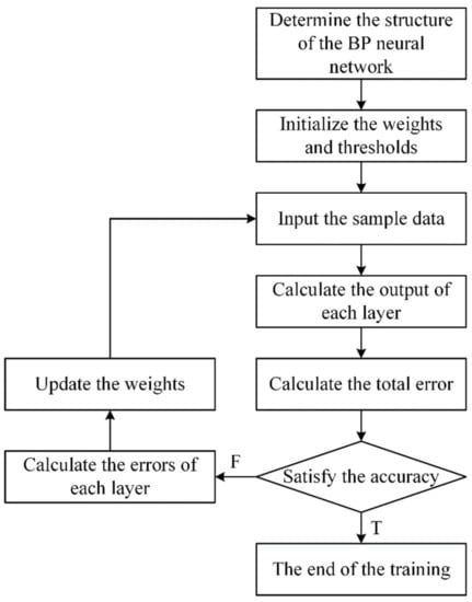
Figure 1.
Flowchart of the BP neural network.
The general steps of the BP neural network model construction include sample selection, sample data normalization, and model establishment.
2.2. Selection of the Sample Data
The accuracy and reliability of the first weighting prediction depend on the understanding of the roof pressure theory. Before mining, the coal seam is balanced with the strata in all directions. After excavating the cut hole, the rock will be deformed due to the destruction of the original stress balance, and a new stress balance will be generated, resulting in the formation of a temporarily balanced rock loosening circle above the roof. The roof weighting refers to the pressure of the hydraulic support supporting the circle. Two main factors affect the roof pressure of the working face: the geological conditions and mining process parameters. The geological conditions mainly include the lithology and thickness of the direct roof and basic roof of the working face, the inclination, and the depth of coal seam and other parameters. The mining technological parameters mainly include the support pattern, the length, width, and mining height of the working face, and the advance speed [22,23,24,25,26].
There is a nondeterministic relationship between the first weighting and the various influencing factors in the coal mine roof, and the influence degree of each factor on the output results is also different. Too many input parameters will affect the speed of the neural network training and bring about some difficulties in data acquisition. Therefore, a correlation analysis of various factors is needed to select the appropriate sample parameters. The gray correlation analysis method is adopted in this paper to analyze the relationships between various factors, which applies to nonlinear problems with complex structures and can be used to conduct a quantitative comparative analysis of a series of dynamic data [27]. The initial sample input parameters chosen are the depth and dip of the coal seam and their varying rates, the length and width of the working face, the thickness of the coal seam, main roof and immediate roof, mining height, advance speed, and roof condition. The output parameters are selected as the initial pressure and periodic pressure. Because the data for the mining height, dip, and coal thickness are only average values and are changing, a simple average value cannot reflect the change of the values, so this paper introduces the rate of change of the mining height ∆S, the rate of change of the dip ∆β, and the rate of change of the coal thickness ∆M.
where , , and are the minimum, maximum, and average values, respectively, of the buried depth;, , and are the minimum, maximum, and average values, respectively, of the coal seam pitch; and , , and are the minimum, maximum, and average values, respectively, of the coal thickness. Table 1 represents a portion of the original data.

Table 1.
The original data.
Because the dimensions and orders of magnitude of each input parameter are different, the input parameters must be dimensionless before conducting the gray correlation analysis [28], and the formula used is Equation (4):
where is the kth dimensionless value of the ith input parameter, is the kth value of the ith input parameter, and m is the total of the ith input parameter. The following formulas are used to analyze the gray correlation degree:
where is the relative difference between the comparison curve and the reference curve at time k, and is the correlation degree of . Table 2 shows the correlation degree table of the first weighting and related influencing factors.

Table 2.
The correlations of the first weighting and related influencing factors.
By analyzing the correlation degree of the factors in the above table, it can be concluded that, apart from the working face length, which has little impact on the mine pressure, the other factors have a significant impact. Therefore, the width of the working face, mining height, advance speed, roof condition of the coal seam, burial depth, thickness and dip of the coal seam, change rate of the inclination angle, burial depth and coal thickness, direct top thickness, and thickness of the main roof are selected as the input parameters for the model training and prediction. The first weighting strength and interval are taken as the output values of the training and prediction of the neural network model.
2.3. Model Parameters
According to the relevant theoretical research on the BP neural network and roof pressure of the working face, we determine the BP neural network model parameters in this paper, including the number of hidden layers, number of hidden layer neurons, initial weights, activation function, expected error, learning rate, and learning times.
- (1)
- The number of hidden layers
Robert Hecht-Nielson proved that a three-layer BP neural network containing only one hidden layer can perform any nonlinear mapping, which can be a mapping from the n dimension to the m dimension. Therefore, the BP neural network prediction model established in this paper is a three-layer BP neural network with only a single hidden layer.
- (2)
- The number of hidden layer neurons
The suitable empirical formula for a BP neural network with a single hidden layer to determine the number of neurons in the hidden layer is shown as follows:
where p and q represent the number of nodes in the input layer and output layer, respectively, and a is a constant whose value range is (1,10).
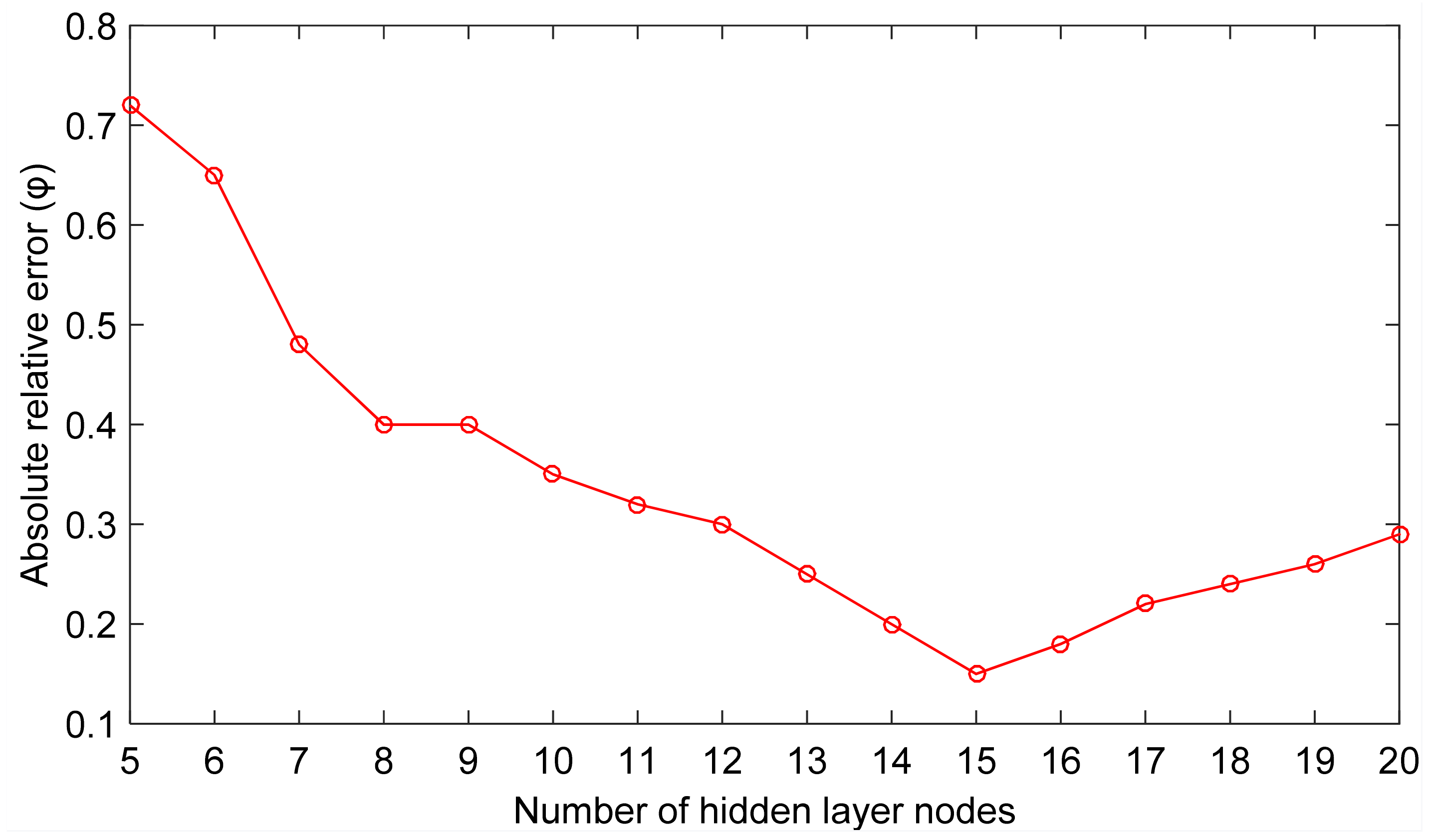
According to the above analysis of the gray correlation degree, the number of input data characteristic values is 12, and the number of output results is 1. Therefore, , and the initial number of neurons in the hidden layer of the BP neural network model established in this paper is 5. After repeated tests, the graph of the relationship between the number of hidden layer nodes and absolute relative errors is shown in Figure 2. The absolute relative error can be obtained from formula 10. It can be seen from the figure that when the number of hidden layer nodes reaches 15, the network output error is minimized.
where is the absolute relative error; and represent the measured results and training results, respectively.
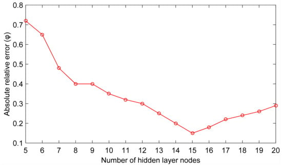
Figure 2.
The errors corresponding to the number of hidden layer nodes.
- (3)
- The initial weights
To avoid the saturation region of the activation function, the weighted sum output value will be near to 0 as much as possible, which can increase the weight adjustment range. Therefore, the initial connection weights are usually random numbers between (−1,1) or (0,2), so that the network will not be greatly affected.
- (4)
- The activation function
The activation function of the hidden layer in this paper is the tansig function, which is found in the MATLAB toolbox, whose value range is (−1,1), which also conforms to the normalized data falling between (−1,1). The output layer selects the purelin function from the MATLAB toolbox, which is linear to increase the value range of the output value. The tansig function is shown below:
where is the base of the natural log function.
- (5)
- The learning rate
According to practical experience, the value range of the learning rate in the BP neural network model is generally between 0.01 and 0.08. In this paper, based on the sample data collected at present, it is concluded by repeated training that when the learning rate is adopted, the performance of the established roof pressure prediction model based on the BP neural network is better.
- (6)
- The expected error
In this paper, the mean square error function is selected in the construction of the BP neural network, and the formula is as follows:
where m represents the number of neurons in the output layer, p is the number of samples, is the true value, and represents the output value of each training iteration.
2.4. Training Results of the BP Model
It can be seen from the above analysis that the number of nodes in the input layer of the model is 12. The input parameters are the inclined length of the working face, advance speed, roof condition of the coal seam, mining height, coal thickness, change rate of the inclination angle, direct top thickness, basic top thickness, burial depth, change rate of the burial depth, coal thickness change rate, and coal seam inclination angle; through repeated tests in this paper, the number of nodes in the hidden layer of the model was determined to be 15; and according to the requirements, the number of nodes in the output layer of the model is set to 1. Sixty sets of data collected from the Datong mining area were selected to establish the model, among which 50 sets were used as training samples and 10 sets were used as prediction samples. The BP neural network model is trained and evaluated by predicting the initial compressive strength and periodic compressive strength of the roof. MATLAB is used in this paper to train the sample data and validate the model. Due to the instability of the BP neural network, the results of each training session are different, so the pressure of the initial weighting and periodic weighting are taken as the target output for 30 training sessions, and the optimal training results are selected as the model obtained by training.
- (1)
- The first roof weighting strength
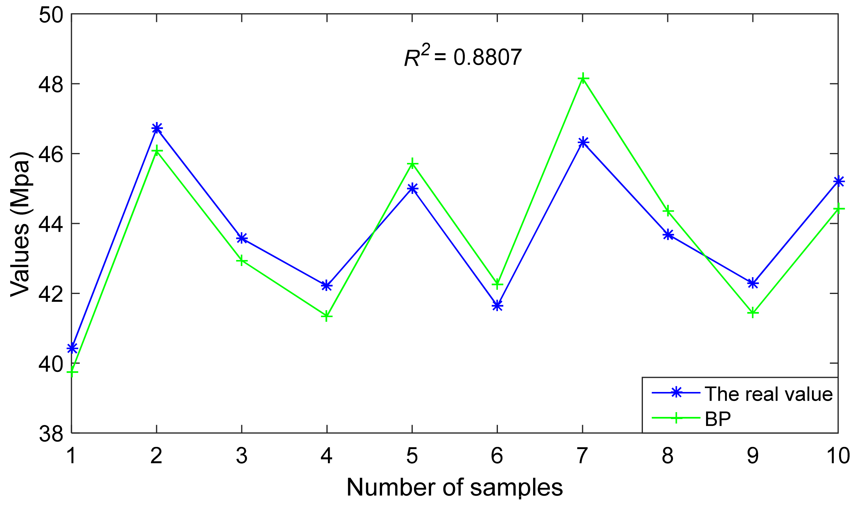
Figure 3 shows the comparison between the predicted value and the real value of the first roof weighting strength predicted by the BP prediction model, which is the best result of the curve fitting between the predicted value and true value in 30 training sessions, with a maximum determination coefficient of 0.8807. The determination coefficient is derived from Equation (13) [29]. The larger the determination coefficient, the better the fit is.
where N is the number of predicted samples, is the predicted value, is the true value, and is the determinant.
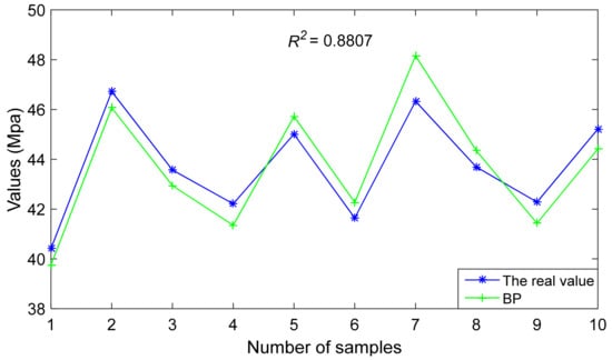
Figure 3.
Comparison of the first roof weighting strength.
- (2)
- Predicting the first roof weighting interval
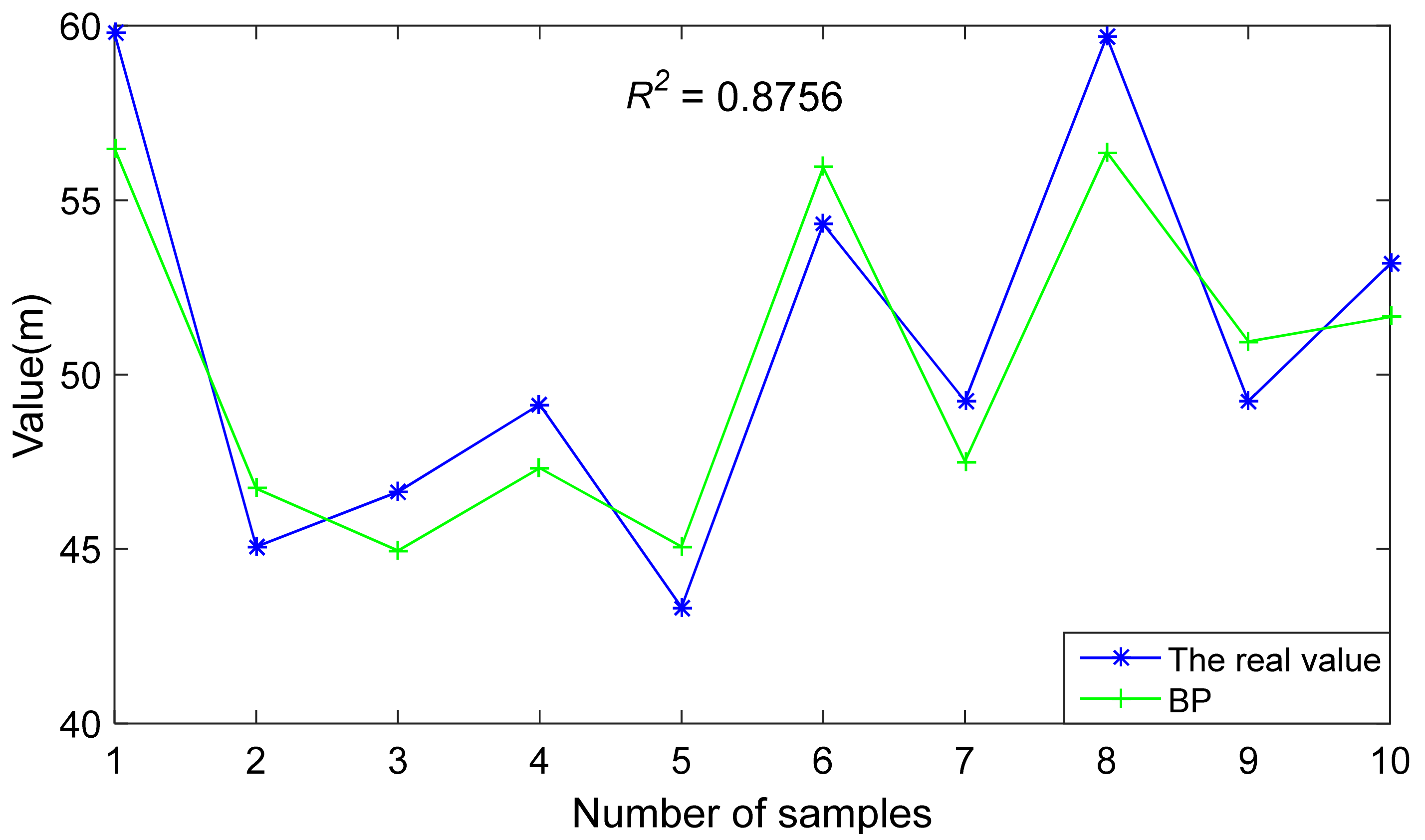
Figure 4 shows the comparison between the predicted value and the real value of the first roof weighting interval predicted by the BP prediction model, which is the best result of the curve fitting between the predicted value and true value in 30 training sessions, with a maximum determination coefficient of 0.8756.
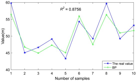
Figure 4.
Comparison of the first roof weighting interval.
It can be concluded from the above diagram that, although the BP neural network model can predict the first weighting strength and first weighting interval of the coal mine roof, the training determination coefficient is small, which indicates that this model is not stable and has a large error. Therefore, this prediction model needs to be optimized.
3. BP Prediction Model of First Weighting Based on the Genetic Algorithm (GA)
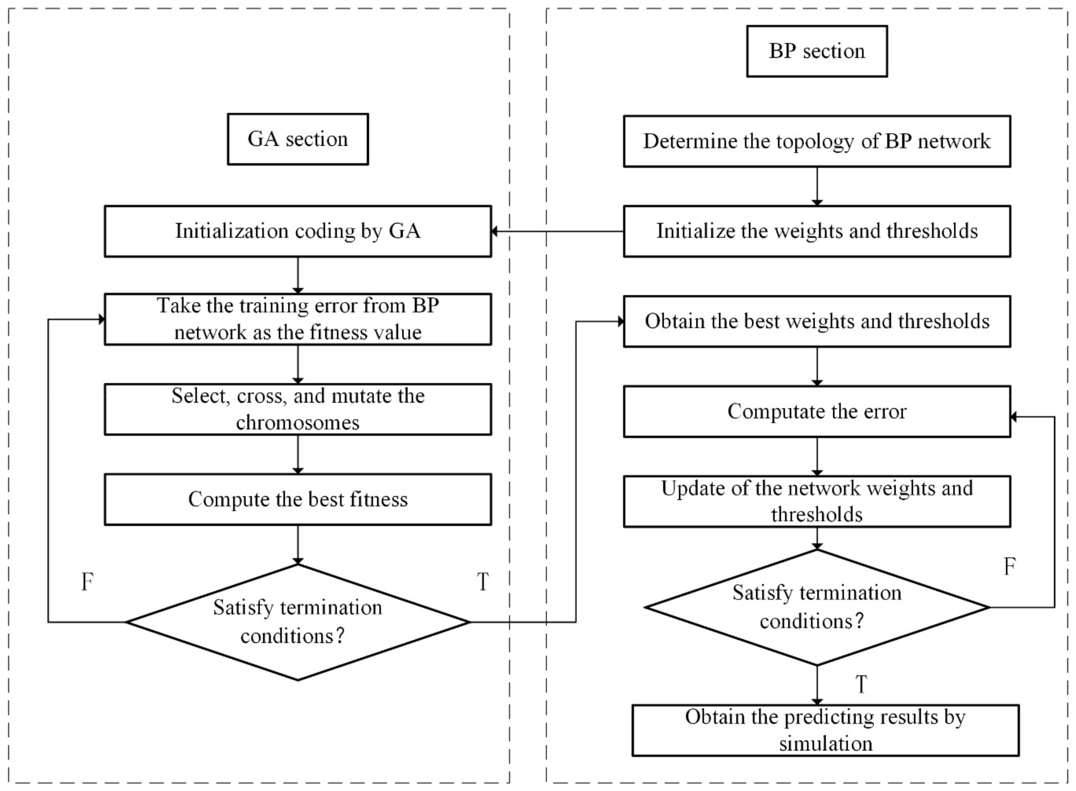
It is necessary to optimize the BP neural network because the volatility of the network is relatively large and it is easy to fall into a locally optimal solution. GA is a domain-independent problem-solving technique, which encodes the problem into a chromosome composed of genes and generates a chromosome representing the solution to the problem through a continuous process of selecting, crossing, and mutating the chromosome. The GA operates on the chromosome code and isolates the characteristics of the problem itself, so it has wide adaptability. At the same time, since the algorithm operates in parallel from multiple initial points, the search process is free from convergence to a local extremum. The GA implements the search process through groups, making it different from a single-point search and easy to parallelize, thus improving the efficiency of the algorithm [30,31]. Therefore, this paper uses a genetic algorithm to optimize the BP network and establish a GA-BP network model. The operational flow of the GA-BP algorithm is shown in Figure 5.
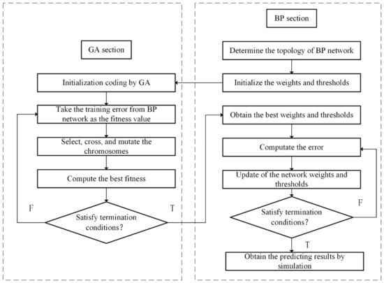
Figure 5.
The flowchart of the GA-BP algorithm.
The optimization of the BP neural network by GA mainly includes determining the structure of the BP neural network and optimizing the weights, thresholds, training, and prediction of the model. Since the optimization of the genetic algorithm is the initial weight and threshold of the BP neural network, as long as we know the topological structure of a neural network, we can determine the number of optimization parameters of the genetic algorithm, to determine the coding length of population individuals. The process of genetic algorithm includes the population initialization, fitness function, selection operator, crossover operator, and mutation operator [32,33].
- (1)
- Population initialization
Through individual binary coding, each individual is represented by a binary string. The network structure of this paper is 12‒15‒1, so the number of weights and thresholds is listed in Table 3.

Table 3.
The number of weights and thresholds.
- (2)
- Fitness function
In this paper, to make the residual difference between the predicted and actual value as small as possible, the sum of the absolute errors between the predicted and actual value of the predicted sample is selected as the output of the objective function.
where n is the number of network output nodes, is the predicted value, and is the true value.
- (3)
- Operator selection
Random ergodic sampling is adopted as the selection operator. A roulette wheel is used to select a pair of individuals; the two individuals compete and the one with the highest fitness is selected.
where n is the number of individuals in the population, is the fitness function value of the ith individual, and is the probability that the ith individual will be chosen.
- (4)
- Crossover operator
The simplest single-point crossover is adopted as the crossover operator. In the individual code string, only one intersection point is randomly selected, and the coding parts of two pairs of individuals are exchanged at that point.
- (5)
- Mutation operator
The mutation operator produces some mutated genes with a certain probability, and the mutated genes are selected randomly. If the selected gene code is 1, it becomes 0; otherwise, it becomes 1. Table 4 shows the parameters of the genetic algorithm.

Table 4.
Parameters of the genetic algorithm.
4. Results and Discussion
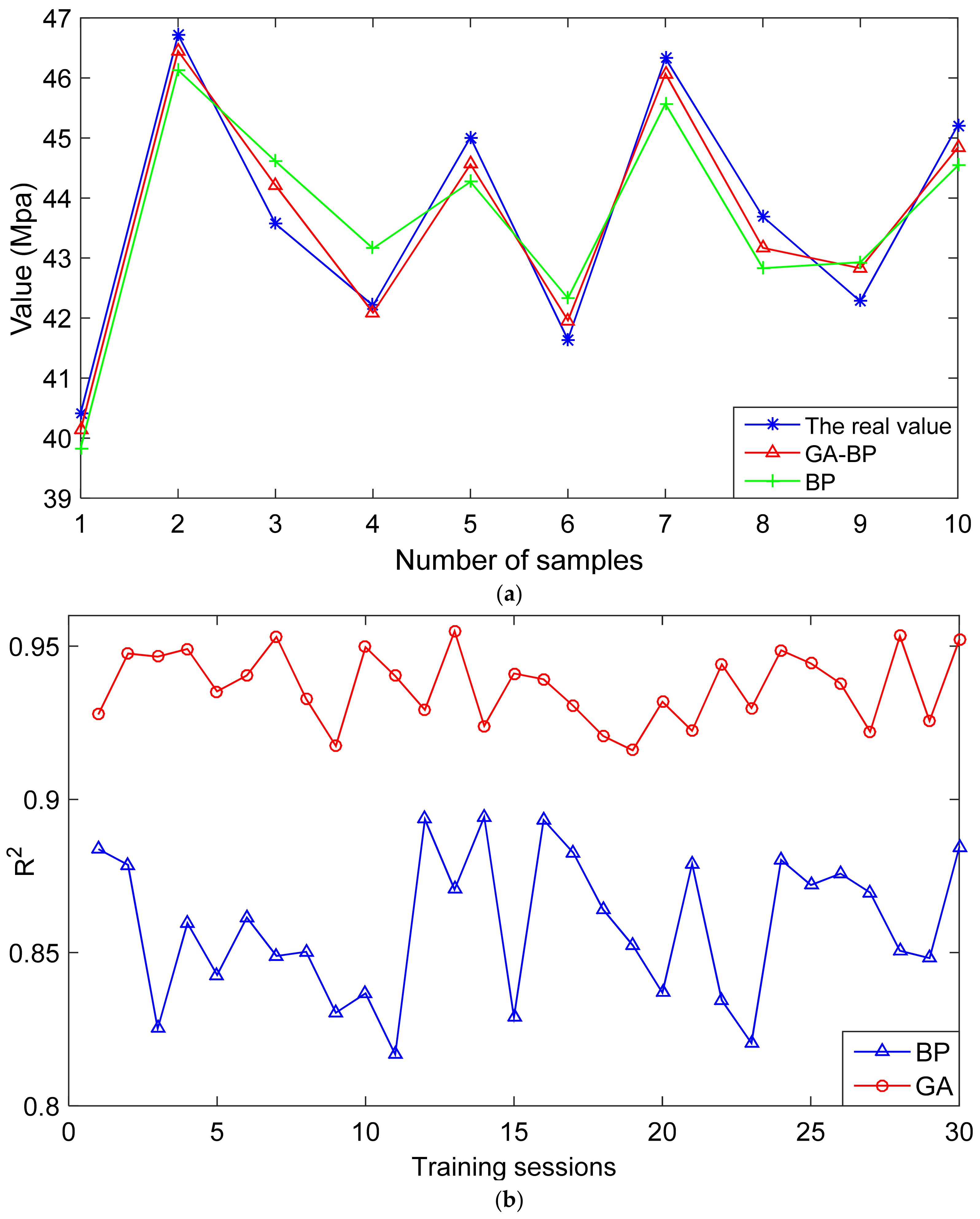
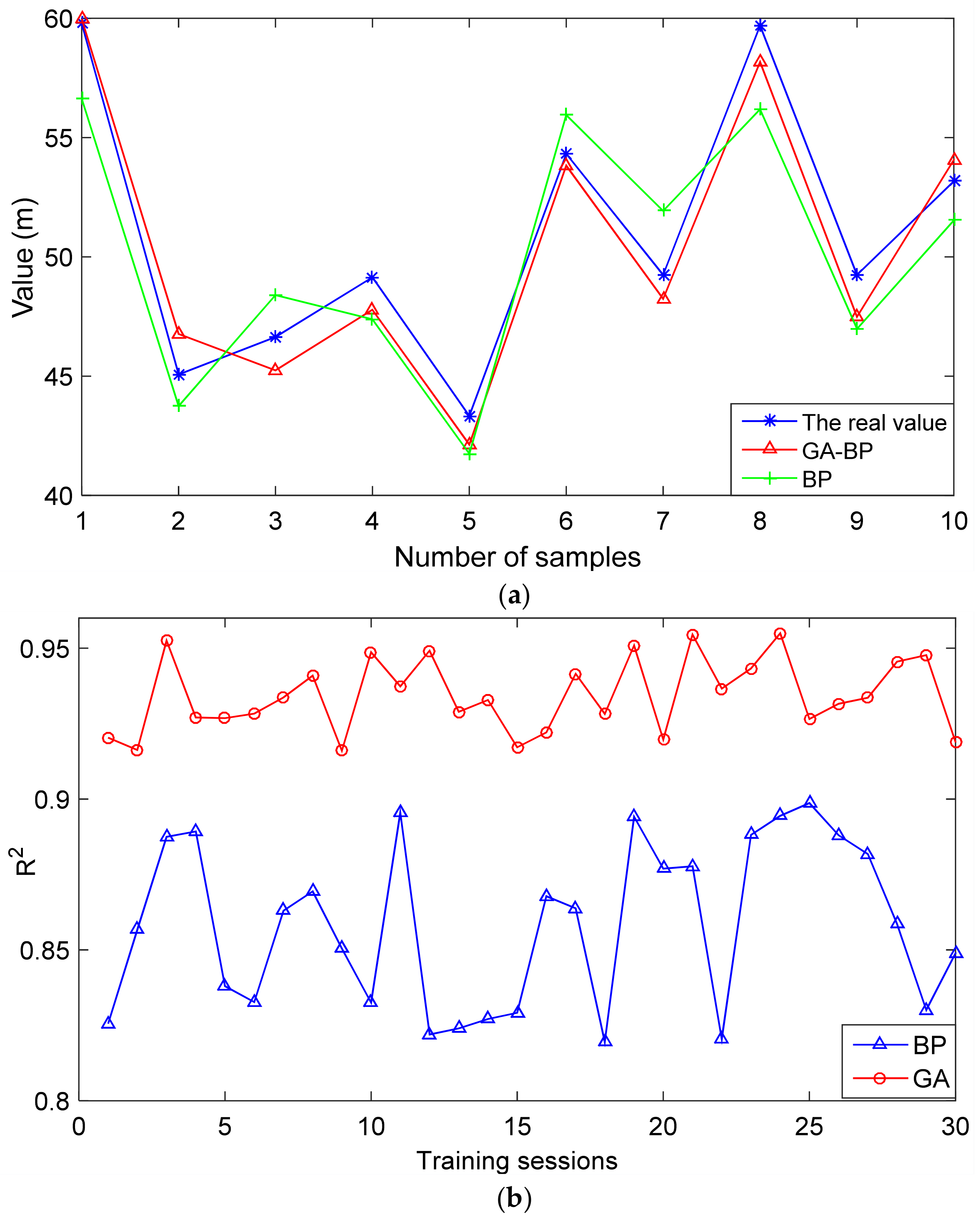
The improved GA-BP model is trained and used to predict the initial compressive strength and interval of the working face roof, and then the predicted results are compared with the predicted results obtained by the BP model above, as shown in Figure 6 and Figure 7.
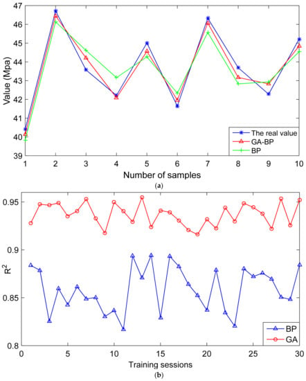
Figure 6.
Comparison of the first roof weighting strength results. (a) The value of the first roof weighting strength predicted by the BP and GA-BP prediction models; (b) a comparison of the determination coefficients predicted by the BP and GA-BP models.
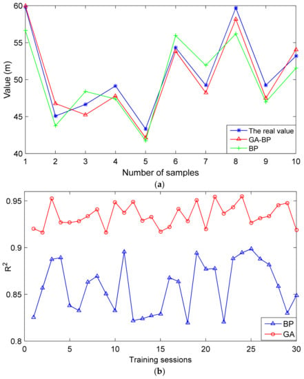
Figure 7.
Comparison of the first roof weighting interval results: (a) the value of the first roof weighting interval predicted by the BP and GA-BP prediction models; (b) a comparison of the determination coefficients predicted by the BP and GA-BP models.
4.1. Comparison of the First Roof Weighting Strength
It can be seen from Figure 6 that the GA-BP model is used to train and predict the initial compressive strength results with a smaller error than that of the BP model, and the GA-BP model has a larger and more stable determination coefficient during the 30 training sessions. The iteration times in Table 5 refers to the number of iterations when the model converges. The iteration times of the GA-BP model and BP model are 21 and 47, respectively, which indicates that the GA-BP model has a faster convergence rate. These results show that the optimized model can better predict the initial compressive strength.

Table 5.
Comparison of the BP and GA-BP models.
4.2. Comparison of the First Roof Weighting Interval
It can be seen from Figure 7 that the GA-BP model is used to train and predict the results of the first weighting interval with a smaller error than the BP model, and the GA-BP model has a larger and more stable determination coefficient during the 30 training sessions. It can be seen from Table 6 that the iteration times of the GA-BP model and BP model are 25 and 53 respectively. This indicates that the GA-BP model has a faster convergence rate. These results indicate that the optimized model can better predict the initial compressive interval.

Table 6.
Comparison of the BP and GA-BP models.
5. Conclusions
In this paper, we used 60 data points from the Datong mining area for the model training and verification, and established a GA-BP model that is suitable for the Datong mining area to calculate the initial pressure strength and a step distance of the roof. The following conclusions can be obtained:
- A lot of influencing factors can be determined in the course of prediction of the first weighting of the working face roof utilizing artificial neural network methods, which can map the complicated nonlinear relation between them.
- The gray correlation degree is used to calculate the relational degrees between the first weighting of the working face roof and various influencing factors in the Datong mining area. The input parameters of the BP prediction model include the width of the working face, mining height, advance speed, roof condition of the coal seam, burial depth, thickness and dip of the coal seam, change rate of the inclination angle, burial depth, coal thickness, direct top thickness, and thickness of the main roof.
- Compared with traditional BP, the BP-GA model has stronger robustness, is available for parallel global searching, and can improve the accuracy of prediction results and the stability of the prediction model.
- We can extend this method of calculating the initial compression strength and step distance to other mining areas. As long as we can collect enough input parameter data, we can train a prediction model that is suitable for each mining area.
Author Contributions
Conceptualization, T.T. and Z.Y.; methodology, T.T. and K.Z.; investigation, F.C.; data curation, F.C. and K.Z.; writing—original draft preparation, T.T.; writing—review and editing, Z.Y.
Funding
This work was supported by the Fundamental Research Funds for the Central Universities [Grant No. 2017CXNL01].
Conflicts of Interest
The authors declare no conflict of interest.
References
- Yuan, X. The Characters andTrend of Accidents in the Coal Mining in China. Dis. Adv. 2012, 5, 866–869. [Google Scholar]
- Duzgun, H.S.B.; Einstein, H.H. Assessment and management of roof fall risks in underground coal mines. Saf. Sci. 2004, 42, 23–41. [Google Scholar] [CrossRef]
- Palei, S.K.; Das, S.K. Logistic regression model for prediction of roof fall risks in bord and pillar workings in coal mines: An approach. Saf. Sci. 2009, 47, 88–96. [Google Scholar] [CrossRef]
- Razani, M.; Yazdani-Chamzini, A.; Yakhchali, S.H. A novel fuzzy inference system for predicting roof fall rate in underground coal mines. Saf. Sci. 2013, 55, 26–33. [Google Scholar] [CrossRef]
- Maiti, J.; Khanzode, V.V. Development of a relative risk model for roof and side fall fatal accidents in underground coal mines in India. Saf. Sci. 2009, 47, 1068–1076. [Google Scholar] [CrossRef]
- Qian, M.G.; Shi, P.W. Mining Pressure and Strata Control; Xu, J.L., Ed.; China University of Mining and Technology Press: Xuzhou, China, 2010; pp. 100–119. [Google Scholar]
- Khandelwal, M.; Kumar, D.L.; Yellishetty, M. Application of soft computing to predict blast-induced ground vibration. Eng. Comput. 2011, 27, 117–125. [Google Scholar] [CrossRef]
- Khandelwal, M.; Singh, T.N. Prediction of blast-induced ground vibration using artificial neural network. Int. J. Rock Mech. Min. Sci. 2009, 46, 1214–1222. [Google Scholar] [CrossRef]
- Monjezi, M.; Ahmadi, Z.; Varjani, A.Y.; Khandelwal, M. Backbreak prediction in the Chadormalu iron mine using artificial neural network. Neural Comput. Appl. 2013, 23, 1101–1107. [Google Scholar] [CrossRef]
- Zhang, H.; Song, J.; Su, C.; He, M. Human attitudes in environmental management: Fuzzy Cognitive Maps and policy option simulations analysis for a coal-mine ecosystem in China. J. Environ. Manag. 2013, 115, 227–234. [Google Scholar] [CrossRef]
- Zhang, R.; Lowndes, I.S. The application of a coupled artificial neural network and fault tree analysis model to predict coal and gas outbursts. Int. J. Coal Geol. 2010, 84, 141–152. [Google Scholar]
- Mohammed, M.; Watanabe, K.; Takeuchi, S. Grey model for prediction of pore pressure change. Environ. Earth Sci. 2010, 60, 1523–1534. [Google Scholar] [CrossRef]
- Doostmohammadi, R.; Moosavi, M.; Araabi, B.N. A model for determining the cyclic swell-shrink behavior of argillaceous rock. Appl. Clay Sci. 2008, 42, 81–89. [Google Scholar] [CrossRef]
- Ambrozic, T.; Turk, G. Prediction of subsidence due to underground mining by artificial neural networks. Comput. Geosci. 2003, 29, 627–637. [Google Scholar] [CrossRef]
- Ashena, R.; Moghadasi, J. Bottom hole pressure estimation using evolved neural networks by real coded ant colony optimization and genetic algorithm. J. Pet. Sci. Eng. 2011, 77, 375–385. [Google Scholar] [CrossRef]
- Winiczenko, R.; Górnicki, K.; Kaleta, A.; Mańkowska-Janaszek, M. Optimisation of ANN topology for predicting the rehydrated apple cubes colour change using RSM and GA. Neural Comput. Appl. 2018, 30, 1795–1809. [Google Scholar] [CrossRef] [PubMed]
- Bashir, Z.A.; El-Hawary, M.E. Applying wavelets to short-term load forecasting using PSO-based neural networks. IEEE Trans. Power Syst. 2009, 24, 20–27. [Google Scholar] [CrossRef]
- Liu, K.; Guo, W.; Shen, X.; Tan, Z. Research on the forecast model of electricity power industry loan based on GA-BP neural network. Energy Procedia 2012, 14, 1918–1924. [Google Scholar]
- Bahadir, E. Prediction of prospective mathematics teachers’ academic success in entering graduate education by using back-propagation neural network. J. Educ. Train. Stud. 2016, 4, 113–122. [Google Scholar] [CrossRef]
- He, Y.; Li, X.L.; Shao, Y.N. Discrimination of varieties of apple using near infrared spectra based on principal component analysis and artificial neural network model. Spectrosc. Spectr. Anal. 2006, 26, 850–853. [Google Scholar]
- Cao, J.C.; Cao, S.H. Study of forecasting solar irradiance using neural networks with preprocessing sample data by wavelet analysis. Energy 2006, 31, 3435–3445. [Google Scholar] [CrossRef]
- Gu, S.; Yao, B. Study on strata behavior regularity of 1301 face in thick bedrock of Wei—Qiang coal mine. In IOP Conference Series: Materials Science and Engineering; IOP Publishing: Bristol, UK, 2017; Volume 231, p. 12108. [Google Scholar]
- Li, J.; Huang, Y.; Zhang, J.; Li, M.; Qiao, M.; Wang, F. The influences of Key Strata compound breakage on the overlying strata movement and strata pressure behavior in fully mechanized caving mining of shallow and extremely thick seams: A case study. Adv. Civil Eng. 2019, 2019, 1–11. [Google Scholar] [CrossRef]
- Lin, G.-Q.; Song, E.-B. The measurement of underground pressure regulation in Ulan Moron coal mine. In 2014 International Conference on Mechanics and Civil Engineering (icmce-14); Atlantis Press: Paris, France, 2014; Volume 7, pp. 287–291. [Google Scholar]
- Zhao, J.; Liu, L.; Zheng, Z. Law of strata pressure behavior in shallow coal seam. In IOP Conference Series: Earth and Environmental Science; IOP Publishing: Bristol, UK, 2018; Volume 113. [Google Scholar]
- Zhu, B.; Li, G.; Kou, W.; Li, H. Simulation of strata behaviour laws of a coal mine in Jungar Coalfield. In Proceedings of the 3rd International Symposium on Mine Safety Science and Engineering, Montreal, Canada; 2016; pp. 651–654. [Google Scholar]
- Liu, S.F.; Xie, N.M. Grey System Theory and Application; Science Press: Beijing, China, 2010; pp. 42–132. [Google Scholar]
- Yang, B.; He, L.B. Establishment and analysis of two normalization methods for backscattering intensity data. Acta Oceanol. Sin. 2018, 40, 145–151. [Google Scholar]
- Gocic, M.; Motamedi, S.; Shamshirband, S.; Petkovic, D.; Sudheer, C.; Hashim, R.; Arif, M. Soft computing approaches for forecasting reference evapotranspiration. Comput. Electron. Agric. 2015, 113, 164–173. [Google Scholar] [CrossRef]
- Whitley, D. A genetic algorithm tutorial. Stat. Comput. 1994, 4, 65–85. [Google Scholar] [CrossRef]
- Leung, Y.W.; Wang, Y.P. An orthogonal genetic algorithm with quantization for global numerical optimization. IEEE Trans. Evol. Comput. 2001, 5, 41–53. [Google Scholar] [CrossRef]
- Liu, C. Price forecast for gold futures based on GA-BP neural network. In Proceedings of the 2009 International Conference on Management and Service Science, Wuhan, China, 20–22 September 2009; pp. 1–4. [Google Scholar]
- Tahmasebi, P.; Hezarkhani, A. A hybrid neural networks-fuzzy logic-genetic algorithm for grade estimation. Comput. Geosci. 2012, 42, 18–27. [Google Scholar] [CrossRef] [PubMed]
© 2019 by the authors. Licensee MDPI, Basel, Switzerland. This article is an open access article distributed under the terms and conditions of the Creative Commons Attribution (CC BY) license (http://creativecommons.org/licenses/by/4.0/).


