Article

Predicting Student Grades Based on Their Usage of LMS Moodle Using Petri Nets

Department of Informatics, Faculty of Natural Sciences, Constantine the Philosopher University in Nitra, 94974 Nitra, Slovakia
*
Author to whom correspondence should be addressed.
Appl. Sci. 2019, 9(20), 4211; https://doi.org/10.3390/app9204211
Submission received: 21 August 2019 / Revised: 1 October 2019 / Accepted: 3 October 2019 / Published: 9 October 2019

Abstract

:
This paper deals with the possibility of predicting student’s grades based on their usage of Learning Management System (LMS) Moodle. It is important to know what materials would be best suited in LMS as study materials and what materials could be improved or removed based on the student’s usage of the materials and the final grade. In order to do this, the correlations between access to materials and the final grade were observed. These correlations could also be used to predict the grades of the student. Therefore, a model with Petri nets was created that based on the highest correlation would be able to predict what grade the student would get based on his usage of LMS. Obviously, it would not be possible to predict every result with certainty, however, more precise predictions could be obtained with higher correlations.

1. Introduction

The implementation of new technologies and practices into education currently represents the greatest support for the development of learner’s cognitive and intellectual abilities. A virtual university system enables to create a virtual classroom on the web. Such systems combine learning management skills with student collaboration capabilities to support learning abilities such as exercises, discussions and grading. Due to the increasing popularity of distance learning, a number of software tools for distance learning for web browsers have been developed. These systems have been used at various universities and departments.
The static structure of information on the web, whose task is to provide information, has long been succeeded. More and more web software systems are being created that are more complex than ever. From a usage point of view of these systems, the need to enrich the information space of the heterogeneous resources under which these systems work is becoming increasingly important, with elements of user adaptation and/or user experience. The goal is to present personalized information to the user, in other words, information that is relevant to the user in a way that is best suited for that user [1].
This paper focuses on the educational processes that happen inside the Learning Management System (LMS) Moodle. The open-source LMS Moodle is useful for creating an effective online learning community. It also encourages learners to participate in the learning process and helps teachers who aim to improve the learning performance of their students through creative collaboration [2].
Moodle (Modular Object-Oriented Dynamic Learning Environment) is an open source LMS developed in Australia in 2002 and has been available since the 1.0 version was released in March 2011. Moodle is used for blended learning, distance education, flipped classroom, and other e-learning projects in schools, universities, workplaces, and other sectors [3]. As a famous learning LMS, Moodle is a diversified technical tool that supports an evaluation of blended learning. Authors in the paper Engaging Asian students through game mechanics: Findings from two experiment studies [4] used Moodle to report the effects of game mechanics to foster users’ engagement in blended learning and found that the digital implementation of game mechanics automatically kept track of students’ activities in Moodle. Moodle provides a number of ways to express and share the knowledge that learners possess. Moodle also provides a good tool for monitoring community learning activities. Through these collaborative activities, learners can create new knowledge on their own and further develop critical thinking and flexible creative problem-solving skills through mutual cooperation between members [5].
The Moodle LMS is customized and has several features available for teachers to assist them in teaching. The LMS is generally used for delivering course content, course progression plan, grading, creating activities, collecting course feedback, and communicating with course participants. Among several features, only a few of them such as assignment, feedback, quiz, and workshop modules are considered very essential and are heavily used [6].
The aim of this paper is to use modeling with Petri nets to predict the student’s success based on his/her passage through the e-course and thus to design models that could be used to create better e-courses for LMS Moodle.

2. Related Work

The introduction of information and communication technologies (ICT) into practice has brought changes in all areas of society including in the field of education [7]. However, in order to fully utilize the potential of these technologies, a new approach to education is needed. This, in turn, requires a new model of the educational institution whose processes would be changed by the use of ICT [8]. Without changing the existing educational process, it is unlikely to achieve a different learning outcome. Information and Communication Technologies have become one of the pillars of modern society and a natural part of the everyday life of most people. Education is no exception. Today, the use of ICT in education varies depending on the countries and types of educational institutions, as well as between institutions. However, the use of technology is a standard in most universities. Examples include LMS and Virtual Learning Environments (VLE) [9].
The great potential of these methods lies in the ability to open the black box and “see” what education actually looks like in online learning environments. Although the use of LMS in teaching is relatively common in many colleges, teachers using LMS in their classroom often do not have many opportunities to see exactly what is happening in their online courses, how students behave, or how they access online materials or progress when engaging in learning activities. Generally, LMS does not automatically include advanced data acquisition tools, while the external data acquisition tools are too complex for teachers and their features to go beyond what the educator may require [10,11].
Regarding the process extraction, the first reference to the method is defined in the process mining in the first Handbook of Educational Data Mining (EDM) [12] as one of the basic EDM techniques. It was, however, mentioned as a technique that had been used rather sparsely until then, as the existing EDM approaches have rarely focused on the process as a whole [13]. Nevertheless, process mining in education is attracting increased research attention. Its potential use in education has been discussed by Reimann and Yacef [14] among others. Reimann et al. [15] dedicated their critical article to process mining from the perspective of methodological challenges in data-intensive research methods.
A browsing behavior model based on High-Level Petri Nets (HLPN) to generate behavioral patterns for e-learning was written by authors Yi-ChunChang et al. [16]. Many researchers have made great efforts to promote high-quality e-learning environments such as adaptive learning environments, customized/adaptive guidance mechanisms, etc. These studies must collect a large number of behavioral patterns for verification and/or experimentation. Collecting sufficient behavioral patterns usually takes a lot of time and effort. To solve this problem, Yi-ChunChang et al. proposed a Model of Browsing Behavior (B2model) based on High Level Petri Networks to model and generate student behavior patterns.The established behavioral patterns are compared with the actual behavioral patterns collected from primary school pupils. The results confirm that the generated behavioral patterns are analogous to the actual behavioral patterns.
An example of the use of Petri nets in education could be described by authors Balogh et al. in the article The possibilities of using Petri Nets for realization of a universal model of educational process [17]. This work summarized the results obtained from the design, creation and implementation of a universal model of educational processes with the use of Petri nets. Based on the created models in Petri nets, it was possible to verify and simulate individual processes through which the student passes through the e-course in LMS. The universal model was implemented at the Department of Informatics in 2009/2010. The module is used in technically oriented courses, mainly in the field of applied informatics. The results obtained from the use of the module are mentioned in the debate and show that in this way it was possible to find certain rules of behavior of students in the e-course in terms of use and compare them with the created process models. In the resulting effect, it was possible to remove all disturbing elements from the e-courses and make them more efficient and attractive. The universal model of educational processes supported by Petri nets has thus contributed to improve student abilities and skills without them knowing it.
In the article Possibilities of Modeling Web-based Education Using IF-THEN Rules and Fuzzy Petri Nets in LMS and in the book Process Modeling Using Petri Nets, there was an example of a fuzzy Petri network which described the modeling of student knowledge that was used in the following example [18,19].
Serial machines, commonly used to describe the behavior of learning processes, have several limitations in modeling complex processes such as the number of states.Therefore, Petri nets are used for given purposes derived from the expanding modeling capabilities of series machines.
One of the advantages of modeling educational processes using Petri nets is their formal description enriched with graphical representation. It allows the precise and exact specification of the educational process and elimination of design ambiguities, uncertainties and contradictions. In addition to the visual representation, Petri nets also have a mathematical basis that is well used in software tools to specify and analyze computer-based educational processes [20]. The article described the creation of a rule-based model. With TransPlaceSim, the rules could be recovered.
The publication Finding learning paths using Petri nets modeling applicable to e-learning platforms [21] presents an approach to model courses with the help of Petri nets. The method can be used to support the development of electronic learning platforms, such as LMS, allowing student guidance in a decision to achieve a particular goal. This goal can be simple, such as passing a course, or even complex, such as combining different modules from different courses to get a qualification. Each course is characterized by a group of modules and the relationships between them. Each module is represented by a Petri net model, and the structure of the module that represents the course dependency is shifted to the next Petri net. Additional courses or modules can be added as their associated Petri Network models can be easily assigned using additional operations. The contribution of this work lies in the use of common techniques to analyze Petri nets to limit student possibilities to optimize his/her path towards grades and qualifications. A simple example with a scenario of a few courses and modules was used to illustrate the approach.
There are many examples where Petri nets are used to model educational systems. They are used in systems where the teacher becomes the main element of the process of learning, modeling a course or using higher-level Petri nets to group materials in e-learning. The work has focused on creating a complete model of an e-learning system that would provide several courses and modules and it would encourage students to find a specific way to achieve their goals in accordance with their needs [22,23].

The Basic Concept of Petri Nets

Petri Net (PN) is a graphical and mathematical modeling tool that has the advantages of graphical notation and simple semantics [24]. Petri nets designate a wide class of mathematical models that allow modeling and describing control flows and information dependencies within a system.
A PN is a 5-tuple [24,25]: PN = (P,T,A,W,M0), where
  • P = {p1,p2,…,pm} is a finite set of places. A place represents a circle, such as p1,p2 and p3 in Figure 1.
  • T = {t1,t2,…,tn} is a finite set of transitions. A transition represents a bar, such as t1 in Figure 1. The intersection of P and T is an empty set, while the union of P and T is not an empty set, i.e., P∩T = ∅ and T∪P ≠ ∅.
  • A⊆(PxT)∪(TxP) is a set of arcs connecting places and transitions, such as the arrowhead from p1 to t1 depicted in Figure 1.
  • W:A→{1,2,3,…} is a weight function, whose weight value is positive integers. Arcs, i.e., arrowhead, are labeled with weights. For example, in Figure 1, the arrowhead from t1 to p3, which is labeled with “2”, is denoted as W(t1,p3) = 2. When the weight is unity and/or “1”, the label of arc is usually omitted, e.g., W(p1,t1) = 1 is omitted in Figure 1.
  • M0:P→{0,1,2,3,…} is the initial marking. If there are k tokens inside place pi, it is said that pi is marked with k tokens. For example, in Figure 1a, p1 is marked with one token, which is denoted as M(p1) = 1. p2 is marked with two tokens, which is denoted as M(p2) = 2. If Figure 1a is the initial status, the initial marking is denoted as M0(p1,p2,p3) = {1,2,0}.
A transition t is said to be fired if all its input places pi are marked with at least W(pi,t) tokens, where W(pi,t) is called the firing condition of transition t. For example, in Figure 1, the firing conditions of t1 are W(p1,t1) = 1 and W(p2,t1) = 2.
A firing transition t removes W(pi,t) tokens from each input place pi and adds W(t,pj) tokens to each output place pj. For instance, since M(p1) = 1 and M(p2) = 2 have satisfied the firing conditions of t1 in Figure 1a, t1 is fired. After t1 is fired as Figure 1b depicts, t1 has removed W(p1,t1) = 1 token from input place p1 of t1 and W(p2,t1) = 2 tokens from input place p2 of t1, respectively, and then added W(t1,p3) = 2 tokens to output place p3 of t1 [16].

3. Materials and Methods

The aim of the work was to model using Petri nets to predict the student success based on his/her passage through the virtual learning environment and thus to design models that could be used to create better e-courses for LMS Moodle. Based on the created educational models in Petri nets, the individual processes could be verified and simulated that were performed when the student passed through the virtual learning environment. An important phase of the work was the mathematical formalization of created models and the implementation of uncertainties that were found in learning and acquiring knowledge using LMS into the created models. The efficiency of the created models would be verified using statistical methods of cluster and correlation analysis.
Workflow was as follows:
  • A design of student behavior models in a virtual learning environment, i.e., study of materials in individual parts of the course, models of logical functions, loop models, condition models, deadlocks, etc. that could simulate the student behavior in the virtual education system and its subsequent rating.
  • After creating the appropriate educational models, it was possible to create a new e-course and test it with the models created for the e-course.
  • A creation of an e-course from the proposed Petri Network models.
  • After result evaluation of the real e-course using models designed for the e-course, it was possible to find out which parts of the e-course were most used for study and especially which parts contributed the most to the better grades of the students.
Real values, learning outcomes from previous years of student evaluations, could be implemented into created educational models and thus verify and subsequently predict student behavior. Models could be completed that required real student ratings to verify their veracity.
Figure 2 shows how the results of the research were achieved. Using the conceptual models of Petri nets from the previous chapter, an e-course was created that would also deploy in the classroom and an e-course model that would be used to simulate the behavior of students in the e-course. From the e-course, log files would be obtained to know how students behaved in the e-course and which parts they used. In addition, information about students passing the test would be acquired. Predicted results from the e-course model would be obtained and then compared with real results.

3.1. Modeling Uncertainty with Petri Nets

The Uncertainty is present everywhere in the real world as well as in the teaching process. No matter how the student behaves in the e-course, how he/she learns, it is not possible to determine precisely how successful he/she will be in the final exam. Its result is always determined by factors that are not possible to be accurately determined. For this reason, it was appropriate to propose the principle of modeling uncertainties and processes that commonly occur in the real world. This would enable to model situations where the outcome was not precisely predetermined, or situations where the outcome was only a probability and not an obvious truth or falsehood.
So far, if a higher chance of an event using Petri nets was needed to be simulated, one way was to add multiple transitions between the places with higher probability of the given event (Figure 3).
When the weight was added to transitions, the first three transitions could be swapped for one transition with a weight of 3. Then there was a chance that the token would move to P1 is 3:1 [26,27]. The approach was useful in calculating the final probabilities of multiple branched events.
The weights were used in stochastic Petri nets when multiple transitions were active but the firing of one prevented the firing of the others. With the weighted transitions, the model from Figure 3 could be changed to the model from Figure 4.
In Figure 4, transition T0 had a weight of three and a transition T3 had a weight of one. The likelihood that a token would pass from P0 to P1 was the same for both models [28]. For the simple decision example, the probability of a result could be calculated by dividing the weight of the firing transition with the sum of the weights of the concurrently active transitions.
p = w 0 i = 0 n w i
w0 was the weight of the firing transition and, wi was the weight of the i-th active transition. In the case of the parallel models of Figure 5, the probability of the final state depended on the combination of the final state probabilities of all concurrent models.
For concurrent models, the probability of activating two independent transitions was calculated as follows:
p = w 0 w 3 i = 0 n w 0 i j = 0 m w 3 j
w0 was the weight of the first transition, and w3 was the weight of the second transition, where both could fire simultaneously without deactivating each other. w0i and w3j were the weights of the i-th and j-th group of active transition, where the firing of one deactivated others. The transitions for which firing of one deactivated the others were called the group of transitions of transition T. The weight of this transition was called w and the weights of transitions from the group were called ws. Therefore, the previous formula could be generalized to:
p = i = 0 n w i j = 0 m w i j
p was the probability of the state to which the model could get out of the current state by firing the correct transitions, wi was the transition weight of the transition group that fired during this step, and wij was the transition weight from the transition group Ti. The formula only worked where the models were concurrent and independent. If models were linked, other formulas needed to be used. In this case, the problem was the increasing number of possible combinations of active transitions. For the example in Figure 6, it was necessary to use two different types of formulas for two different activation options.
For the model in Figure 6, two different situations needed to be considered: Only independent transitions (T3, T4, T5, T6, T7, T8) would fire, or one dependent transition (T0, T1, T2) and two independent transitions would fire. A dependent transition was one that had more than one entry place.
The sum of weights for all active transitions was defined as:
s = i = 0 n w i
Then, the probability of activating one dependent transition and two independent transitions, such as T0 and T7 or T8, was calculated as:
p = w n s · w i k = 0 n w i k
wn was the weight of the dependent transition, wij was the weight of the independent transition, and wik was the weights of the transition from group Ti.
The probability of firing of all independent transitions was calculated as:
p = i = 0 n w i j = 0 m w i j · s k = 0 o w k s
wi was the weight of the i-th independent transition, wij was the weight of all independent transitions from transition group Ti, and wk was the weight of the dependent transitions.
Another approach that worked for all types of models, but only in the case where the weights were ignored, was to find out all the variants of firing transitions. If the permutations of all possible transition firings were taken, the number of options through which the model could get into the next states would be obtained. Taking into consideration the number of states the model can get into and the sum of the permutations of all the transitions firing, the number of all the transition firings could be obtained. If the numbers were divided now, the probability of that state would be aquired.
p = n ! ( i = 0 m n i ! )
In this case, n was the number of transitions that fired, and ni was the number of transitions that were active for each state acquired from the state [29].

3.2. Observing Student Movement in LMS

Moodle log files were used to track the movement of students in the e-course. Moodle is used for four primary purposes: (1) making course materials available for browsing when describing class contents, (2) performing a quiz during class, (3) referring to an external web page, and (4) submitting a report at the end of the term. To analyze learning history, it is desirable to clarify the purpose of collecting Moodle course logs [30]. Moodle provided an easy way to get student access logs. With just a few clicks in the Moodle administration page, Moodle would export the log files in .csv format. The logs contained:
  • Time
  • User name
  • Affected user
  • Event context
  • Component
  • Event name
  • Description
  • Source
  • IP
Time, user name, event name, and context were essential for the purposes of the research. It was also necessary to remove teacher access from the log files, as they were also written to the log files, but were not needed to model the student behavior. The logs were organized as follows: The main unit was a student. The student contained a session number. Each session contained links to the Moodle logs that displayed which parts of Moodle the student had visited during that session. The sessions were obtained from the Moodle logs. To get a session, the data were organized by name and time. Based on the work [24], an upper time limit was created − θ. Exceeding this time limit meant a new session. If the time on the first page in one session was t0 and the user’s current URL was t, then this page was considered as one session if the inequality t − t0 ≤ θ was true. While for the next page, it was inequality t0 + θ > t.
This was the first page of the next session. Normally, θ was set to 30 min. The time of the following accesses were important. If the following access was created sooner than 45 min from the previous one, it was assumed to be a single session. If the time interval was greater than 45 min, it was a new session. An interval of 45 min was chosen because normally one lesson took 1.5 hours. In this case, if the student did not attend the course at least twice during one lesson, we could assume that they did not use the e-course during that lesson [31,32,33]. Based on these times, the sessions were removed that contained only one entry, as this was not a session but only one login per class.
However, in addition to observing the sections visited, the focus was on the number of visits in the “Book”, “Lecture” and “Assignment” sections. The log files showed that only these items were used by students to study. The aim was to find out how the number of study material visits would affect the final grade of students. First of all, attention was payed to visits to materials used to study the principles of operating systems as the exam itself was largely theoretical.

4. Results and Discussion

After entering the data from log files, grades and attendance into Excel, graphs were obtained that in detail described the following section. In the charts, the correlation between the grade and the number of visits was observed.
In Figure 7, it was obvious what grade the students got based on access to the study materials “Lecture”. The horizontal axis represents the number of visits and the vertical axis the final grade of the student. The lectures were in PDF format. These contained the most information to help students to pass the exam. The correlation of attendance and final ranking was −0.48723, the highest for this section, which represented a moderate correlation rate. The correlation analysis examines the tightness of the statistical dependence between the quantitative variables. The correlation coefficient is the extent of the linear dependence of the two variables. The coefficient is calculated by dividing the covariance with the standard deviation. The value of the coefficient is in the interval from −1 to 1 where −1 represents the indirect proportion, 1 is the direct proportion, and 0 represents the independence of X and Y. According to Cohen, the interpretation of the correlation coefficient is divided from 0.0 to 1.0 (trivial correlation, small, medium, big, very big, almost complete).
Figure 8 presents what grade the students got based on access to the study materials in “Book”. The horizontal axis represents the number of visits and the vertical axis the final evaluation of the student. It was the Book module in Moodle that enabled to easily create multi-page resources with a book-like format. The book module made it possible to divide the curriculum into main chapters and subchapters as this module was intended to be a simple source of information for both students and teachers. It also contained the amount of information required for the test. The correlation of traffic and final ranking for this section was −0.43531, the second-highest, which represented a moderate correlation rate.
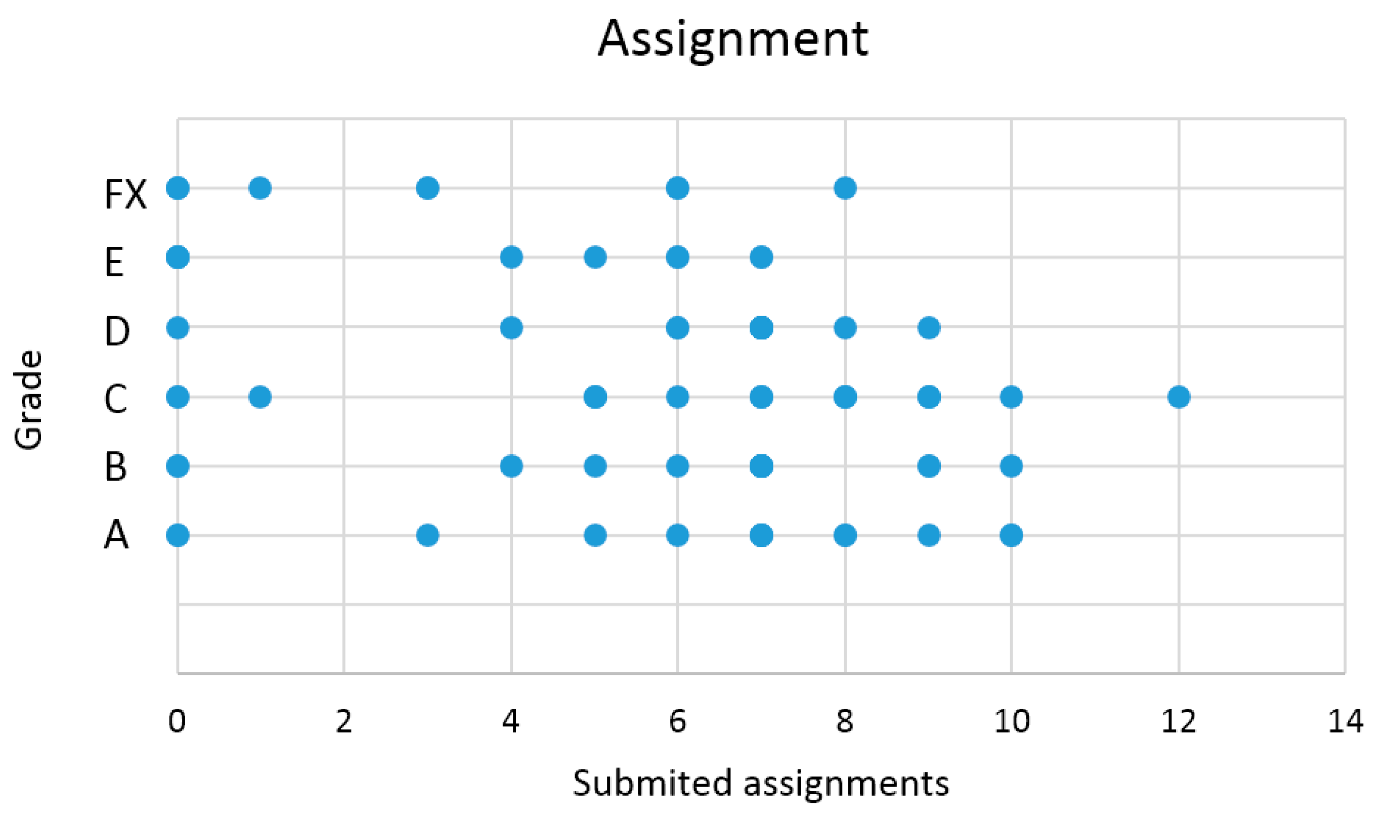
Figure 9 shows what grades students got based on assignments submitted during exercises or at home. The horizontal axis represents the number of submitted assignments and the vertical axis represents the final grade of the student. The correlation for this figure was −0.33359, and the correlation was also classified as a moderate correlation rate.
The last statistic to be observed was the student attendance. For the Figure 10, the correlation was −0.26355, the lowest, which already represented a low correlation rate.

4.1. Model of the Final Exam in Petri Nets

Each student was allowed two attempts for the final exam if he/she failed to pass the exam the first time. Based on student grading, a model in Petri Nets was created that showed how students proceeded with passing the exam.
The “Start” location represented the number of students who took the exam this year. The model (Figure 11) also used transition weights to display the distribution of grades from a single exam. Transitions in which “Exam”, “Exam 2”, and “Exam 3” places were entered, had weights set according to the number of students who received a grade for the exam, as determined by the exit points of these places. In the model, weights were displayed by transition weights so it was shown that four students after the first exam did not come to the next exam, and five students did not take the third exam after failure, but the students who came to the third exam all succeeded. Observing the model, the question arose whether it would be possible to see any improvements in the grade among exams in terms of visits to study materials.
In the model of Figure 12, “Mat 1” and “Mat 2” were added to serve as an e-course visit counter. “The Book” and “Lectures” were the chosen materials to observe. In the previous graphs, they displayed the most significant correlations and they were the only materials that could be used to study between the exams. The tracking data from the model produced interesting results. For students who failed the first attempt, the correlations between their grade obtained after successfully completing the second or third attempt and their time spent studying in the e-course were insignificant. For students who completed the exam after the second attempt, these correlations were −0.24551 for Book visits and −0.13365 for Lecture visits, both of which represented a small correlation. For students who completed the exam on the third attempt, correlations were positive, 0.555851 for “Book” visits and 0.610275 for “Lectures”, which would mean that the less they studied, the better grade they got. It could be assumed that these correlations could be explained by the possibility that students cheated on the test or having only a small sample of students for the test (five students).
For this reason, the students who passed the exam on their first attempt or did not come to the next dates were observed more. For them, the correlation of the final grade and the time spent studying in the course was most striking, as explained below.
For students who succeeded on the first attempt or gave up after the first attempt, correlation based on Moodle“Book” visit was −0.43742. Their arrangement can be seen in Figure 13.
For students who succeeded on the first attempt or gave up after the first attempt, the correlation based on Moodle“Lecture” visit was −0.58561, which represented a greater correlation. This is shown in Figure 14. This was the most significant correlation of all.
To sum up, it is not possible to conclude that the only contributing part to improve student grades was the PDF lectures that students could view in Moodle. Neither participation in the exercises nor the practical assignments submitted to the exercises had a significant impact on the final evaluation of students.

4.2. Model of Grade Prediction

Based on the obtained graphs, it could be presumed that the parameter that influenced the students’ success the most in the final exam was their visit in “Lectures” material in Moodle. Therefore, the graph in Figure 14 was created.
The graph shows what final grade students received when they accepted the course. According to the number of hits, they could be divided as follows:
In the first row of Table 1, there are ranges of visit counts. They were obtained from Figure 14 by looking at the ranges of visits in “Lecture” material for each grade. The maximum range was determined by the highest visit number for that grade, and the minimum was determined by the last visit number that did not figure for a lower grade. The second row shows the number of students for the given lecture visit ranges. The numbers of students who received a certain grade for a given number of visits can be seen in the rest of the table. Based on the table, the following model of Petri nets could be created:
From the start place (Figure 15), the token got to one of the categories selected based on the number of student visits to the lecture. These places were selected according to the graph in Figure 14. In this model, transition weights were used that were set according to the number of students assigned to the categories. Subsequently, the token got to the grade place through a transition whose weight was set according to the number of students in the given visit range who received the grade. Using the model, it was possible to simulate the prediction of student grades based on their access to the lecture material [34].
The probability of selecting a category and consequently the probability of selecting a grade for that category was calculated using Formula (8).
p = w a i = 0 n w i
wa was the weight of the fired transition, wi was the weight of the i-th transition, n was the number of active transitions, and p was the final probability.

5. Conclusions

The aim of the paper was to propose a way of predicting student success based on his behavior in Moodle. The method of predicting the student’s grade could also be used to modify the course or the method of grading students based on the correlation between the attendance of study materials and the grade. If there was a significant impact of one type of study material on the final grade, it could be assumed that it was these study materials that helped the students to master the curriculum the most. If an activity did not have a significant impact on the student’s grade, it might be removed or there would be an option to explore why the activity did not affect the student’s grade.
The method of predicting the grade from the paper could be used for any type of material in the LMS with any correlation between the use of the material and the final grade. However, for lower correlations, it would not be possible to predict the grade with sufficient accuracy, so it was recommended to use the method for materials for which the correlation was the highest. This article gave a suggestion of a way of predicting student success based on this behavior in Moodle. Together with the method of grading students based on the correlation between the attendance of study materials and the grade, it could also be used to modify the course.

Author Contributions

Conceived and designed the experiments, Z.B.; performed the experiment, M.K.; analyzed the experimental data, Z.B. and M.K.; validation, Z.B.; data curation, M.K.; writing—review and editing, Z.B.; methodology, Z.B.; supervision, Z.B.; project administration, Z.B.; The manuscript was written and approved to submit by all authors.

Acknowledgments

This paper was created with the financial support of the project KEGA 036UKF-4/2019, Adaptation of the learning process using sensor networks and the Internet of Things.

Conflicts of Interest

The authors declare no conflict of interest.

References

  1. Holub, M.; Bieliková, M. An inquiry into the utilization of behavior of users in personalized Web. J. Univers. Comput. Sci. 2011, 17, 1830–1853. [Google Scholar]
  2. Kim, E.; Park, H.; Jang, J. Development of a Class Model for Improving Creative Collaboration Based on The Online Learning System (Moodle) in Korea. J. Open Innov. Technol. Mark. Complex. 2019, 5, 67. [Google Scholar] [CrossRef]
  3. Costello, E. Opening up to open source: Looking at how Moodle was adopted in higher education. Open Learn. J. Open Distance e-Learn. 2013, 28, 187–200. [Google Scholar] [CrossRef]
  4. Hew, K.F.; Huang, B.; Chu, K.W.S.; Chiu, D.K. Engaging Asian students through game mechanics: Findings from two experiment studies. Comput. Educ. 2016, 92, 221–236. [Google Scholar] [CrossRef]
  5. Zhou, L.; Chen, L.W.; Fan, Q.M.; Ji, Y.L. Students’ Perception of Using Digital Badges in Blended Learning Classrooms. Sustainability 2019, 11, 18. [Google Scholar] [CrossRef]
  6. Kc, D. Evaluation of Moodle Features at Kajaani University of Applied Sciences—Case Study. Procedia Comput. Sci. 2017, 116, 121–128. [Google Scholar] [CrossRef]
  7. Molnar, G. The Impact of Modern ICT-Based Teaching and Learning Methods in Social Media and Networked Environment. In Proceedings of the 11th International Scientific Conference on Distance Learning in Applied Informatic (DiVAi), Sturovo, Slovakia, 2–4 May 2016; Wolters Kluwer Cr a S: Strašnice, Czechia, 2016; pp. 341–350. [Google Scholar]
  8. Molnár, G.; Benedek, A. ICT related tasks and challenges in the new model of technical teacher training. In Proceedings of the Eighth International Multi-Conference on Computing in the Global Information Technology (ICCGI), Nice, France, 21–26 July 2013; IARIA: Barcelona, Spain, 2013; pp. 40–44. [Google Scholar]
  9. Juhaňák, L.; Zounek, J.; Rohlíková, L. Using process mining to analyze students’ quiz-taking behavior patterns in a learning management system. Comput. Hum. Behav. 2019, 92, 496–506. [Google Scholar] [CrossRef]
  10. Romero, C.; Cerezo, R.; Bogarín, A.; Sánchez-Santillán, M. Educational process mining: A tutorial and case study using Moodle data sets. In Data Mining and Learning Analytics: Applications in Educational Research; John Wiley & Sons, Inc.: Hoboken, NJ, USA, 2016; pp. 1–28. [Google Scholar]
  11. Romero, C.; Ventura, S. Educational data mining: A review of the state of the art. IEEE Trans. Syst. Man Cybern. Part C (Appl. Rev.) 2010, 40, 601–618. [Google Scholar] [CrossRef]
  12. Romero, C.; Ventura, S.; Pechenizkiy, M.; Baker, R.S. Handbook of Educational Data Mining; CRC Press: Boca Raton, FL, USA, 2010. [Google Scholar]
  13. Trcka, N.; Pechenizkiy, M.; van der Aalst, W. Process mining from educational data. In Handbook of Educational Data Mining; CRC Press: Boca Raton, FL, USA, 2010; pp. 123–142. [Google Scholar]
  14. Reimann, P.; Yacef, K. Using process mining for understanding learning. In Handbook of Design in Educational Technology; Routledge: Abingdon, UK, 2013; pp. 472–481. [Google Scholar]
  15. Reimann, P.; Markauskaite, L.; Bannert, M. e-R esearch and learning theory: What do sequence and process mining methods contribute? Br. J. Educ. Technol. 2014, 45, 528–540. [Google Scholar] [CrossRef]
  16. Chang, Y.-C.; Huang, Y.-C.; Chu, C.-P. B2 model: A browsing behavior model based on High-Level Petri Nets to generate behavioral patterns for e-learning. Expert Syst. Appl. 2009, 36, 12423–12440. [Google Scholar] [CrossRef]
  17. Balogh, Z.; Turcani, M.; Magdin, M. The possibilities of using Petri Nets for realization of a universal model of educational process. In Proceedings of the 2013 IEEE 14th International Conference on Information Reuse and Integration (IRI), San Francisco, CA, USA, 14–16 August 2013; pp. 162–169. [Google Scholar]
  18. Balogh, Z.; Turcani, M. Possibilities of Modelling Web-Based Education Using IF-THEN Rules and Fuzzy Petri Nets in LMS. In Informatics Engineering and Information Science, Pt I; AbdManaf, A., Zeki, A., Zamani, M., Chuprat, S., ElQawasmeh, E., Eds.; Springer: Berlin, Germany, 2011; Volume 251, pp. 93–106. [Google Scholar]
  19. Klimeš, C.; Balogh, Z. Modelovanie Procesov Pomocou Petriho Sietí; Fakulta prírodných vied; UKF Nitra: Nitra, Slovakia, 2012. [Google Scholar]
  20. Kucharik, M.; Balogh, Z. Evaluation of fuzzy Petri nets with the tool TransPlaceSim. In Proceedings of the 10th IEEE International Conference on Application of Information and Communication Technologies (AICT), Baku, Azerbaijan, 12–14 October 2016. [Google Scholar]
  21. Campos-Rebelo, R.; Costa, A.; Gomes, L. Finding learning paths using Petri nets modeling applicable to e-learning platforms. In Proceedings of the 3rd IFIP WG 5.5/SOCOLNET Doctoral Conference on Computing, Electrical and Industrial Systems, DoCEIS 2012, Costa de Caparica, Portugal, 27–29 February 2012; Volume 372, pp. 151–160. [Google Scholar]
  22. Chen, S.M. Representing fuzzy knowledge using extended fuzzy Petri nets. In Proceedings of the 2nd International Symposium on Uncertainty Modeling and Analysis, College Park, MD, USA, USA, 25–28 April 1993; pp. 339–346. [Google Scholar]
  23. Mtibaa, S.; Tagina, M. A Petri-Net model based timing constraints specification for e-learning system. In Proceedings of the 2012 International Conference on Education and e-Learning Innovations, Sousse, Tunisia, 1–3 July 2012. [Google Scholar]
  24. Murata, T. Petri Nets: Properties, Analysis and Applications. Proc. IEEE 1989, 77, 541–580. [Google Scholar] [CrossRef]
  25. Jensen, K. Colored petri nets. Lect. Notes Comput. Sci. 1987, 254, 248–299. [Google Scholar] [CrossRef]
  26. Kodamana, H.; Raveendran, R.; Huang, B. Mixtures of Probabilistic PCA with Common Structure Latent Bases for Process Monitoring. IEEE Trans. Control Syst. Technol. 2019, 27, 838–846. [Google Scholar] [CrossRef]
  27. Tian, Y.; Wang, X.Z.; Jiang, Y.; You, G.H. A Distributed Probabilistic Coverage Sets Configuration Method for High. Density WSN; Ieee: New York, NY, USA, 2017; pp. 2312–2316. [Google Scholar]
  28. Dehban, A.; Jamone, L.; Kampff, A.R.; Santos-Victor, J. A Deep Probabilistic Framework for Heterogeneous Self-Supervised Learning of Affordances; Ieee: New York, NY, USA, 2017; pp. 476–483. [Google Scholar]
  29. Kuchárik, M.; Balogh, Z. Modeling of Uncertainty with Petri Nets. In 11th Asian Conference on Intelligent Information and Database Systems (ACIIDS 2019); Nguyen, N.T., Gaol, F.L., Nguyen, N.T., Trawinski, B., Hong, T.P., Eds.; Springer: Berlin, Germany, 2019; Volume 11431, pp. 499–509. [Google Scholar]
  30. Dobashi, K. Automatic data integration from Moodle course logs to pivot tables for time series cross section analysis. In Knowledge-Based and Intelligent Information & Engineering Systems; ZanniMerk, C., Frydman, C., Toro, C., Hicks, Y., Howlett, R.J., Jain, L.C., Eds.; Elsevier Science Bv: Amsterdam, The Netherlands, 2017; Volume 112, pp. 1835–1844. [Google Scholar]
  31. Fang, Y.; Huang, Z. An improved algorithm for session identification on web log. In Proceedings of the 2010 International Conference on Web Information Systems and Mining (WISM 2010), Sanya, China, 23–24 October 2010; Volume 6318, pp. 53–60. [Google Scholar]
  32. Benko, L.; Reichel, J.; Munk, M. Analysis of student behavior in virtual learning environment depending on student assessments. In Proceedings of the 13th IEEE International Conference on Emerging eLearning Technologies and Applications (ICETA), Stary Smokovec, Slovakia, 26–27 November 2015. [Google Scholar]
  33. Maheswara Rao, V.V.R.; Valli Kumari, V.; Raju, K.V.S.V.N. An intelligent system for web usage data preprocessing. In Proceedings of the 1st International Conference on Computer Science and Information Technology, CCSIT 2011, Bangalore, India, 2–4 January 2011; Volume 131, pp. 481–490. [Google Scholar]
  34. Štencl, M.; Štastný, J. Neural network learning algorithms comparison on numerical prediction of real data. In Proceedings of the 16th International Conference on Soft Computing Mendel, Brno, Czech Republic, 23–25 June 2010; pp. 280–285. [Google Scholar]
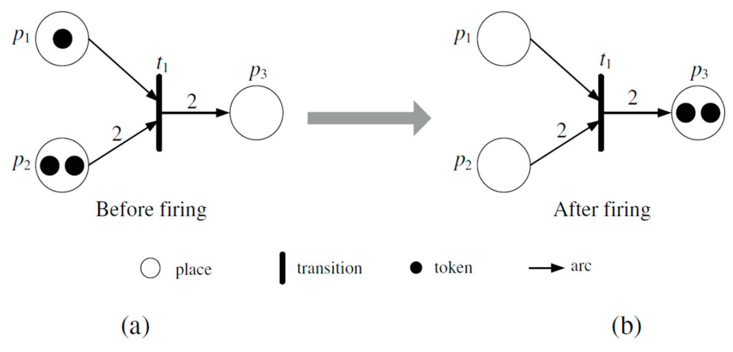
Figure 1. Example of Petri Nets: (a) Before firing tokens, (b) After firing tokens [16].
Applsci 09 04211 g001
Figure 2. Conceptual model.
Applsci 09 04211 g002
Figure 3. Example of a Petri Net model with random selection.
Applsci 09 04211 g003
Figure 4. Petri Net model with weighted transitions.
Applsci 09 04211 g004
Figure 5. Petri Net model with concurrent parts.
Applsci 09 04211 g005
Figure 6. Petri Net model with concurrent parts.
Applsci 09 04211 g006
Figure 7. Grades based on visits in “Lecture” materials.
Applsci 09 04211 g007
Figure 8. Grades based on visits in “Book” material.
Applsci 09 04211 g008
Figure 9. Grades based on visits in “Assignment” material.
Applsci 09 04211 g009
Figure 10. Grades based on attendance.
Applsci 09 04211 g010
Figure 11. Model of the final exam in Petri Nets.
Applsci 09 04211 g011
Figure 12. Model of the final exam with the observation of the study.
Applsci 09 04211 g012
Figure 13. Grades based on visits in “Book”material, at the first attempt.
Applsci 09 04211 g013
Figure 14. Grades based on visits in “Lecture”material on the first attempt.
Applsci 09 04211 g014
Figure 15. Model of grade probability for a single student.
Applsci 09 04211 g015
Table 1. The number of students based on lecture visits and final grade.
Visits0..45..121314..1718..2930..56
Students22186264
A052024
B212040
C641200
D411000
E610000
FX400000