Deep LSTM with Reinforcement Learning Layer for Financial Trend Prediction in FX High Frequency Trading Systems


STMicroelectronics S.r.l.–ADG Central R&D Group, 95121 Catania, Italy
Appl. Sci. 2019, 9(20), 4460; https://doi.org/10.3390/app9204460
Submission received: 13 September 2019
/
Revised: 15 October 2019
/
Accepted: 17 October 2019
/
Published: 21 October 2019
(This article belongs to the Special Issue Advanced Bio-Inspired Mathematical Modeling and Machine Learning Algorithms for Quantitative Finance Applications)
Abstract
:High-frequency trading is a method of intervention on the financial markets that uses sophisticated software tools, and sometimes also hardware, with which to implement high-frequency negotiations, guided by mathematical algorithms, that act on markets for shares, options, bonds, derivative instruments, commodities, and so on. HFT strategies have reached considerable volumes of commercial traffic, so much so that it is estimated that they are responsible for most of the transaction traffic of some stock exchanges, with percentages that, in some cases, exceed 70% of the total. One of the main issues of the HFT systems is the prediction of the medium-short term trend. For this reason, many algorithms have been proposed in literature. The author proposes in this work the use of an algorithm based both on supervised Deep Learning and on a Reinforcement Learning algorithm for forecasting the short-term trend in the currency FOREX (FOReign EXchange) market to maximize the return on investment in an HFT algorithm. With an average accuracy of about 85%, the proposed algorithm is able to predict the medium-short term trend of a currency cross based on the historical trend of this and by means of correlation data with other currency crosses using techniques known in the financial field with the term arbitrage. The final part of the proposed pipeline includes a grid trading engine which, based on the aforementioned trend predictions, will perform high frequency operations in order to maximize profit and minimize drawdown. The trading system has been validated over several financial years and on the EUR/USD cross confirming the high performance in terms of Return of Investment (98.23%) in addition to a reduced drawdown (15.97 %) which confirms its financial sustainability.
1. Introduction
The key to correctly identifying market trend is to correctly estimate both medium-term and long-term trends. Analyzing the financial time-series we can see that many trends follow well-established dynamics in which it is possible to identify recurrent graphic patterns. However, often trading systems are interested not only in identifying the current trend but rather in identifying those ‘latent signals’ generated by the market and that in fact constitute the first notices of a trend change. Usually, a change of trend in any financial market is preceded by a so-called transitional period of indefinite duration but in any case short to which a trend reversal will follow [1]. Obviously, if this is true for the stock or bond market, it is even more so for the foreign exchange market (Forex), which obviously involves much greater volumes of financial transactions than stocks [2,3,4,5]. Many trading algorithms try to identify the current trend and therefore the signals of inversion through a correlation study between the analyzed financial instrument and others related to it because listed in the same market segment or for other reasons of a financial nature. One of the ways in which many traders exploit these correlations is related to the so-called ‘arbitrage’. In financial markets, arbitrage can occur when trying to get an advantage of differences in the price of single currency related to short-time misalignments between the traded currency with the related ones [2]. In the foreign exchange market, this approach would seem to be worthy of further investigation as it has been noted that many currency changes perform with very correlated dynamics also in terms of sharing an exchange rate (see for example EUR/USD cross currency with EUR/GBP or EUR/USD with GBP/USD). Figure 1 shows an example of related financial time-series (EUR/USD with GBP/USD).
To the above we add the observation that the foreign exchange market presents strongly non-linear and non-stationary cross dynamics influenced by macroeconomic factors, national and international monetary policies, military conflicts, etc. These factors, more often than not unpredictable, generate a certain level of uncertainty and non-predictability which obviously will have a greater impact in the long term and are more contained in the short term if the trading system policy provides appropriate financial compensation or loss-cutting algorithms based on prudent use of dynamic stop-losses. For these reasons, the author propose the implementation of a high frequency trading (HFT) algorithm that allows fast and rapid financial transactions to be performed with the undoubted advantage of containing losses in the case of incorrect trades although this is counterbalanced by the consequent finding that even profit can only be contained. Obviously, this last aspect will also be compensated by the execution of a large number of transactions and by a careful trading strategy based on the robust identification of the medium-short term trend. The author has already investigated the development of HFT algorithms both in the stock market and in the currency market, through deep learning methods based mainly on the use of supervised learning architectures such as long short-term memory (LSTM) networks. The results obtained were satisfactory also due to both the high predictive nature of the proposed algorithm and the grid strategy applied in the Forex market [1,2].
However, in the literature several authors have investigated the use of deep learning and reinforcement learning (RL) methodologies in order to structure efficient trading systems. Below are some scientific contributions that show the advantages that can be obtained from the use of supervised deep learning and RL based algorithms.
1.1. Deep Learning (LSTM) and RL Based Trading Systems: Literature Review
In [6], the authors proposed an interesting trading approach based on the usage of deep reinforcement learning. The authors proposed a trading agent based on deep reinforcement learning, to autonomously make trading decisions by means of a modified deep Q-network (DQN) and actor-critic (A3C) approach. They implemented a deep framework based on the use of a stacked denoising autoencoders (SDAEs) and LSTM) in order to design a robust mechanisms to make the trading agent more practical to the real trading environment. The results confirmed the effectiveness of the proposed approach [6].
In [7], a multi-objective intraday trading method is proposed. The key idea of the proposed approach is the usage of multi-objective deep reinforcement learning methodology for intraday financial signal representation and trading. The authors in [7] implemented a deep neural network to extract market deep features followed by a reinforcement learning framework (with ad-hoc LSTMs) able to make continuous trading decisions. In order to get a good trade-off between profit and risk, the authors proposed a multi-objective optimization approach which includes two objective function (one for profit and one for risk) with different weights. The experimental results confirmed that the approach reported in [7] is effective even though a drawdown analysis is not included in the paper.
In [8], Chen et al. proposed an innovative method based on the concept of ‘energy trading’. Through an ad-hoc mathematical model of energy trading strategies of a prosumer in the proposed holistic market model, the prosumer’s decision-making process will be analyzed as a Markov decision process so that the local market participation will be solved by deep reinforcement learning technology with experience replay mechanism. This approach can be easily extended to financial markets with specific reference to the stocks of companies in the field of energy management. One of the most-studied indicators in quantitative finance is certainly the financial volatility. There are several ways to heuristically calculate the volatility of a particular financial instrument. Several trading systems are based on the estimation of volatility factor of the financial instrument so that it is very important to have a robust and efficient method for volatility prediction.
In [9], the authors proposed a pipeline for volatility prediction of such currency pair (INRUSD). By means of recent deep LSTM architectures, the volatility of INR/USD currency pair has been successfully estimated. The research reported in [9] proposed an innovative approach to forecast uptrend or downtrend movement of daily volatility. The authors compared LSTM based algorithm with classical regression neural networks, SVM, random forest, regression algorithms, decision trees, and boosting techniques. The LSTMs-based approach was confirmed to be the best performing one.
In [10], the authors analyzed several trading strategies based on deep learning based approaches applied to trade the Shanghai Composite Index. The result of the survey in [10] confirmed that the best trading strategy based on the use of deep neural network is the ones which shows high predictive accuracy in low volatility market, as it can help investors on reducing the risk while obtaining satisfactory returns. In [11], Chen et al. proposed a very interesting idea: cloning the previous trading strategy stored in the financial records to make profitable trading system. Anyway, due to the large amounts of financial data extracting its decision logics and key-features of the performer trading strategies are particularly difficult. For these reasons, the authors proposed in [11] to use a reinforcement learning (RL) system to mimic professional performer trading strategies. The authors designed the RL environment (states, actions, and rewards) In order to apply ad-hoc policy gradient method able to imitate the expert’s trading strategies. The experimental results show that the proposed RL pipeline is able to reproduce around 80% of the well-performing trading decisions both in training and validation sessions.
1.2. Deep Computing-Based Trading Systems: Literature Review
In [12], the authors proposed an interesting approach named based on A-trader system (multi-agent system for stock trading). The authors analyzed the application of deep learning approaches in the A-trader framework for making profitable trading strategies in the forex market. The analyzed deep learning H20 algorithm seems the more performed according to the experimental results reported in [12]. In [13], the authors analyzed and compared such machine learning approaches with a novel ones proposed by the authors and based on the usage of 1D convolutional neural network (CNN). The proposed one-dimensional convolutional layers process different financial data such as prices and volume, extracting deep features instead to be used for making the trading strategies. The authors evaluated their method’s performance with full back-testing session of the proposed trading pipeline on historical data of six futures from January 2010 to October 2017. The results seem very promising [13]. For many years, several authors have studied the chaotic behavior of such phenomena, including the financial market dynamics [14].
Lee in [14] proposed a Chaotic Type-2 Transient-Fuzzy Deep Neuro-oscillatory Network (CT2TFDNN) for worldwide financial data prediction including major cryptocurrencies, forex, major commodities, and several financial indices. The author introduced the novel concept of chaotic neural oscillators which serves as ‘transient-fuzzy input neurons’ of the used deep neural network. This proposed deep network was used by the author to forecast the trend of the traded instrument. The experimental results confirmed that the proposed approach is very promising.
In [15], the authors analyzed the use of “trailing” method for making efficient trading strategies. More in details, the authors in [15] proposed a novel price trailing method considering the trading problem as a control problem. The proposed method implemented robust agents that can withstand large amounts of time-series noise, identifying the price trends in order to perform profitable operations. The P&L curve reported in [15] confirmed that the proposed approach performs very well in the financial market. Anyway, as per most of the trading strategies proposed in literature, the approach reported in [15] s well as most of the above described, although they perform very well, they lack an accurate analysis of both maximum and dynamic drawdown [1,2], which is necessary to correctly evaluate the proposed trading strategy as it allows to quantify well the investor’s exposure risk in addition to the necessary capital exposure to refer to implement the proposed strategy.
In this paper, the author proposes a pipeline which exploits the advantages of the recent deep learning and reinforcement learning methods combined with the instrument correlation study, in order to predict the medium-short term trend and therefore perform fast operations (HFT) in order to maximize profit (gain) and minimize risk (drawdown). The method will first be described in the next section (Materials and Methods) as well as the dataset used for testing and validation the proposed approach. In the Section 2.4, the grid trading system based on the trend predictions performed by the deep learning and RL block will be illustrated. Therefore, the results will be presented in Section 3 in which they will be commented highlighting advantages and future developments of the proposed pipeline.
2. Materials and Methods
The method proposed in this paper will seek to exploit the correlations between distinct currency crosses in order to predict the medium-term trend of ones of them. To this end, the authors will describe below a pipeline that is based on the use of set of cross-currency exchanges characterizing an arbitrage opportunity in the Forex market. As introduced in the first section, an arbitrage takes advantage of differences in the price of single currency related to short-time misalignments between the traded currency with the related ones [16]. A typical example of arbitrage is the so-called triangular arbitrage referred to three currencies of which one is obtainable from the combination of the prices of the other two crosses. In this article, we will refer to the EUR/USD, GBP/USD, and EUR/GBP crosses. A similar approach can be extended to any other trio of related currencies. The currency on which to execute trading operations is EUR/USD [13]. The price of the EUR/USD cross for arbitrage purposes in the currency market must always be obtainable from the other two pairs EUR/GBP and GBP/USD by the relationship
In Equation (1), we have denoted with px(tk) the price of the currency. Therefore, in a financially balanced market, so that an investor cannot take advantage of arbitrage conditions and consequently obtain a systematic gain, Equation (1) must always be verified, i.e., there must be a very precise temporal correlation between specific currency crosses. In reality, small short-term misalignments are always found in the Forex markets and these are often excellent trading opportunities for financial robot advisors who automatically execute many operations, taking advantage of these short-time market misalignments. The author is investigating the design and use of specific hand-crafted features (which the author has already used in the medical field) extracted from the chart of currency time-series and which would seem to early indicate the possible misalignments between the cross currency prices from which are extracted [17,18,19,20,21].
For the reasons mentioned above, the author has designed a pipeline which, to determine the medium-term trend of a given currency, analyzes the correlations between the related currencies in the context of a triangular arbitrage. In the specific case, without losing generalization, the author will refer to the EUR/USD currency as that on which to execute financial trading operations and to the EUR/GBP and GBP/USD currencies to determine the data set for a possible triangular arbitrage. Similar considerations can be extended to any other set of currencies with the same financial characteristics.
Having established this necessary premise, the author will describe the proposed pipeline below. Figure 2 below shows the block diagram of the algorithmic pipeline that is intended to be described in this paper:
The following paragraphs will illustrate each of the blocks present in the complete diagram of the proposed pipeline and shown in Figure 2.
2.1. Data Pre-Processing Block
The objective of this block is to pre-process the data of the incoming financial time-series. Specifically, in this block the data of the incoming time-series will be normalized in the range [0, 1]. Figure 3 shows an example of normalized financial time-series relating to the three cross currency analyzed in this paper. In this way, whatever the pricing of the cross currency entering our system, the pipeline will always process data in the range [0, 1], greatly improving the stability of the proposed algorithm.
In order to train and validate the proposed pipeline, the author has organized a proper dataset of financial pricing data. Specifically, historical financial data (with 99.9% accuracy) of EUR/USD, GBP/USD, EUR/GBP for the years 2004–2018 have been collected. Again, with reference to the aforementioned time period, for each cross currency the historical data referring to the opening and closing prices, higher and lower in addition to the time of each quotation (CET time) have been collected. This dataset has been properly divided in order to organize a set of data that can be used for the training phase of the proposed system and the remaining for the testing and validation session. Specifically, such training simulations and annual validation have been performed, dividing the dataset as follows: 70% of the mentioned dataset was used to train the pipeline, while the remaining 30% was used to validate and test the proposed method. Both the training set and the validation ones has been analyzed as to understand if the possible trends (LONG, SHORT, NULL) were equally represented in both datasets in order to avoid overfitting issues for the deep learning system.
The financial data thus organized are therefore presented as input to the pre-processing system described in this section whose output will be further processed by the next deep learning block.
2.2. Deep Learning Block
The goal of this block is to determine a first prediction of the medium-short term trend for the currency to be traded, in the case of this article, we will refer to the EUR / USD cross. The architecture that the author wanted to use in this work is based on the use of deep long short-term memory (LSTM) networks. An exhaustive description of the LSTM architecture can be found in [22,23]. The LSTMs architectures are basically particular types of recurrent neural networks (RNN) with a marked ability to learn long-term dependencies. LSTMs have many variations. The fundamental unit of an LSTM network is the cell. A cell consists of three data ports (input, forget, output) that process the data using a sigmoid type activation function “σ” while the cell input and status are transformed with “tanh” activation [22]. The cell is able to store (recall) values over arbitrary time intervals while above gates are able to manage the input/output data flow of the cell.
The following Figure 4 shows a classical LSTM structure with a specific detail about the simple cell unit.
The following Figure 5 reports the typical LSTM cell as used in the architecture proposed in this paper.
The mathematical model that characterizes the dynamics of the single LSTM cell is
where
- represent the LSTM weights
- represent the used biases for each cell
- represents the cell state
Therefore, during the data processing phase performed by the LSTM network, the input data (the set of financial time-series of the cross currency chosen to define a triangular arbitration) will be properly processed by means of the equations defined above, establishing—in simple words—which dynamics of input data keep in memory and discard (forget gate). More details on the LSTMs architectures in [24].
LSTM architectures can be used effectively to classify signals or in general data on input [25,26]. For these reasons, the author has equipped the proposed LSTM based deep pipeline with a fully-connected neuronal layer with a SoftMax layer and a classifier in cascade. The final classification layer uses the probabilities returned by the SoftMax activation function for each input to assign the input to one of the mutually exclusive classes and compute the loss and performance indexes. In this way, our pipeline will be able to process the input data (financial currency time-series) through the LSTM cells therefore to appropriately classify the features thus generated through the SoftMax layer and classifier. A similar classification pipelines have been used effectively by the author in appropriately classifying both signals and images albeit in different areas than the financial one here described [27,28,29,30,31]. This confirms that the approach of cascading a SoftMax block with classifier to a deep network capable of extracting features from input data (LSTMs, convolutional neural networks, auto-encoders, etc.) is certainly robust as well as performing with regard to discriminative capacity [32].
The proposed deep architecture is composed of the following elements:
- Input layer;
- LSTM layer (HiddenCellNumber);
- LSTM layer (HiddenCellNumber);
- FullyConnected Layer (NumberClasses);
- SoftMaxLayer
- ClassificationLayer
In the proposed pipeline the variable HiddenCellNumber defining the number of cell for each LSTM layer is 300 while NumberClasses is 3 i.e.: (0): representing SHORT trend; (1) representing LONG trend; (2) representing no trend as the currency is in ‘trading range’, as is commonly said in financial jargon, to indicate that the financial instrument does not have a well-defined trend.
In the proposed pipeline, the input time-series for each currency cross is divided in the following way: a well-defined part of length will be used as input sequence for the deep pipeline described above while the subsequent quotations (of a length equal to that used for the input sequence) will be used to establish the financial trend of the currency which one intends to predict. In the present case, we will consider the length of the financial time-series segment, a number of quotations equal to 100 candlesticks for each incoming currency. Considering that we are interested in HFT trading algorithms, we used a one-minute (1M) timeframe for each currency cross. The prices of the quotations refer to the closing prices of each financial candlestick. The currency of which we intend to predict the trend is the EUR/USD while, as mentioned, the three triangular arbitrage currencies are EUR/USD, EUR/GBP, and GBP/USD. Therefore, for every 100 quotations of the closing prices of the three currencies mentioned above, the deep learning system described above will process these data providing a predictive estimation of the trend of the next 100 quotations (closing price) relative to the currency you are chosen to trade i.e., EUR/USD. Figure 6 shows the described learning process.
The predicted trend made by LSTM based system will be fed to next block, i.e., the RL correction block.
2.3. RL Correction Block
The goal of this block is to implement a correction/verification of the currency trend predicted by the previous deep learning block as the tests performed show that the performance of the previous block is not high. In fact, considering for example the quotations with 1M timeframe of the three analyzed currency crosses for the year 2018, the accuracy of the previous block in relation to the prediction of the EUR/USD instrument trend stands on average at 70%, as evident from the trend of the learning/validation curve shown in Figure 7 below.
For these reasons, the author has equipped the algorithm with an additional learning layer based on an unsupervised deep learning policy based on reinforcement learning (RL) techniques. Below in Figure 8 the pipeline that it has been implemented in this block.
As can be seen from Figure 8, the core of the reinforcement learning (RL) framework used to improve the performance of the entire trend forecasting pipeline is based on a motor map architecture. These architectures are none other than SOM networks consisting of a layer of input synaptic weights to which a layer of output synaptic weights is mapped which, in certain aspects, emulates the biological action of the motor cortex that has a corresponding sensory estimate (input layer of the motor map) maps a given action by stimulating the motor neurons by means of the motor cortex (motor map output layer). The motor map learning algorithm is of the winner-take-all (WTA) type with updated neighborhood for the input layer while it is of the "random-driven" type for the output layer. More details on the configuration of the Motor Maps and the applications that these non-supervised learning systems have in different fields of science, see the articles reported in [28,32].
We proceed to the description of the RL algorithm described in Figure 8. Let us indicate with Wkin (x, y) and with Wout (x, y) the matrices of the syntactic input and output weights of the RL Motor Map used in the algorithm proposed in this article. A 900-cell RL motor map was used, arranged in a 30 × 30 lattice structure. Both layers are randomly initialized. While the input synaptic weights can assume real values, the output weights Wout (xk, yk) can assume only the following discrete values: 0,1,2 as, as mentioned, they will be associated with the external stimulus which in our case corresponds to the trend to predict or 0: SHORT Trend, 1: LONG Trend, 2: Trading range.
At each learning time, the portion of time-series of the three currencies used for the learning of the previous block is presented, in this case, the three triangular arbitrage currencies, i.e., EUR/ USD, GBP/USD, and EUR/GBP. The three price carriers (closing price) properly normalized will be presented to the input level of the RL motor map. For each neuron of the input layer, a distance d(x,y) will therefore be determined between the respective synaptic input weights of the neuron with the time-series values used to determine the trend to be predicted for the EUR/USD currency, in the case that is being analyzed here. Formally, the determination of a matrix of a distances d(x,y) of 30 × 30 dimension (corresponding to that of the lattice structure used for the RL motor map) will take place.
Having obtained this matrix of distances d(x, y) as per Equation (2), we will select the neuron that minimizes this distance, i.e., the one whose syntactic weights are closest according to the adopted metric (Euclidean), to the input signals (the portion of financial currency time-series). We denote by (xmin, ymin) the coordinates of the neuron that contains the minimum distance d(x, y).
Now consider the corresponding position (xmin, ymin) in the output layer of the RL motor map. Well this will produce a specific value of the syntactic weight of output wout (xmin, ymin) which therefore corresponds to the value of the trend that the network expects for the next N quotations of the closing price of the EUR/USD currency (with N = 100 in the case which is described here). In practice, we will obtain the result of
At this point, the RL system will consider the state st of the system (xtmin, ytmin, dt(xtmin, ytmin), wtin (xtmin, ytmin), wtout (xtmin, ytmin), ,, , N, trendp-Deep Learning) to determine the optimal policy Pt to be implemented in order to predict the correct mid-term (N = 100 quotes) trend of the EUR/USD currency. We have therefore added the "t" apex to the variables used up to now in order to indicate their value to the learning step "t" corresponding to the state st We defined with trendp-Deep Learning the output predicted trend provided by previous deep learning block. The problem is shown below in a formal manner. We defined an ‘action’ at as the most likely medium-term trend of the EUR/USD currency referred to the next 100 close price quotations. We defined an ‘agent’ and selected the action (at). We are interested in determining the optimal policy (Po) that minimizes the cumulative discount reward
Where γ is a proper discounted coefficient in (0,1). The reward function R(.) defined to address the issue of determining the most likely medium-term EUR/USD trend is
where the terms ) respectively represent the prediction error of the trend committed by the previous deep learning block and by the current output wtout (xtmin, ytmin) of the RL motor map, determined as
The policy P0 consists therefore in verifying –at each step- the trend predicted by the previous deep learning block with respect to the prediction performed by the output synaptic weight of the RL motor map network, thus confirming the best prediction, that is the one that minimizes the reward determined above or proceeding to a ‘random’ update of the syntactic weight in order to determine a new prediction trend that instead can minimize the reward in the following steps and during the learning phase. Specifically, the agent will apply a policy P0 able to provide the actions
Obviously, in the case where the trend prediction is wrong both in the previous deep learning block and in the current RL motor map system, the proposed approach will proceed with the update of the output weight as
Once this phase has been determined, we will proceed to update the synaptic input weights if and only if the prediction of the RL motor map system was correct, that is, only if the following options occurred:
In situations where Equations (16) are verified, the input weights of the winner neuron, i.e., the neuron at (xtmin,ytmin) coordinate will be updated accordingly, bringing them closer to the dynamics shown by the cross currency time-series portions presented in input. In this way we intend to train the RL motor map network to recognize specific dynamics in the financial input patterns in order to activate the appropriate corrections to the prediction performed by the previous deep learning block. The input weights will be updated as
where represents the learning rate (defined as , represents a function that provides the close price quotations of the EUR/USD cross currency time-series being used as input data of the RL motor map while represents the update function of the neighborhood of the winning neuron that in the case under examination has been implemented by the classic adaptive Gaussian function [25,29].
The following Figure 9 shows the decreasing dynamic of the defined reward function during the learning phase of the RL motor map trend predictor:
The overall prediction system, i.e., the deep learning block with correction made by RL framework, is able to increase the overall average accuracy in trend prediction to about 85% confirming the robustness and effectiveness of the proposed approach. Table 1 shows the validation results of the proposed trend-forecasting pipeline described in Figure 8, both with the trend correction performed by the RL system and without it.
It is clear that, in terms of accuracy, the trend prediction system based only on the deep learning block (Figure 6) performs less than the system corrected with the RL pipeline (Figure 8). This is evident in the various years in which the proposed forecast pipeline has been tested, in relation to the EUR/USD currency cross.
2.4. Currency Trend Forecast Application: HFT Grid Trading System
In the previous sections, the forecast pipeline of the medium-term trend of a currency has been described based on the analysis of the correlated currency dynamics through a financial technique known as triangular arbitrage (both through deep learning methodologies and through reinforcement learning techniques). Once the forecast robustness of the trend in the medium term has been established (we have defined without loss of generalization, an average trend defined by 100 quotations on 1M timeframe) it is now necessary to plan a trading strategy that based on such forecasts, can execute a series of financial transactions (trades) agree with the estimated trend. For this application, the author intends to use the HDT algorithm with the grid already effectively used and illustrated in a previous work published in this journal [2]. We make a brief reference to this type of trading system which in all respects can be counted among the HFT algorithms.
Basically, a grid trading strategy is an algorithm that seeks to make profit on the market movements of the underlying financial instrument by positioning properly time-spaced buy and sell orders (grid distance). In our case, the trading system will work as follows.
Using the prediction system of the trend just described in the previous sections, a medium-term trend will be generated, i.e., for the next N quotations (in our case N = 100 has been hypothesized without loss of generalization of the method). Based on this predicted trend, the grid trading system as described in paper [2] will open operations in accordance with the predicted trend (buy for a predicted LONG trend; sell (or short selling) for a predicted SHORT trend ) and appropriately spaced according to the adaptive grid methodology illustrated in detail in the algorithm implemented in [2] and which will basically avoid opening up close positions with each other if the overall drawdown of the financial portfolio is increasing (therefore mediating ‘the loss’ with operations of the same sign appropriately spaced) and vice versa will attempt to open closer positions (dynamically reducing the distance of the grid) if the drawdown is decreasing. In the event that the pipeline produced will provide a trading range forecast (no well-defined forecasted trend), the trading system will not execute any operation entering the hold status. As described in previous sections, we perform trading operations on EUR/USD cross. The next paragraphs report the results of the testing phase of the proposed approach (trend forecast with grid trading system) which will confirm the efficiency of the proposed method beyond any reasonable doubt.
3. Discussion and Conclusions
We have accurately validated our pipeline using a complete and comprehensive dataset. To this end, as described in Section 2.1, ad-hoc financial dataset has been properly organized. The cross-currency dataset was downloaded from the Tickstory website [33] and—as specified—contains 1M timeframe quotes (99.9% accuracy) of the EUR/USD, GBP/USD, EUR/GBP cross currencies for the years 2004–2018. As mentioned in Section 2.1, we performed training simulations and annual validation, dividing the training set as follows: 70% of the data has been used as training set while the remaining 30% were used to validate and test the proposed pipeline. The simulations were performed on an AMD Ryzen 16 Cores server with Nvidia RTX 2080 Ti GPU supporting CUDA operations and in MATLAB 2018b full toolboxes. We supposed a broker account with 30,000.00 US dollars as the initial balance and 2 pips of bid/ask spreads (the spread is average gain cashed by the broker). We supposed an account leverage of 1:400 and a LOT size for each single FX trade order. The following indexes are defined in order to provide a benchmark comparison with similar Forex trading systems [2]
The proposed approach has been validated over all available years (from 2004 to 2018) performing several tests selecting different daily time-window which means a different stock exchange [2]. Table 2 shows the benchmark comparison of the proposed approach with respect to similar ones proposed in literature (for each comparison the author has used the same forex currency dataset as per cited method):
Regarding the performance in terms of the HFT system, the proposed method performs many more operations than the previous approach developed by the authors [2]. The increase in the number of trading transactions related to the fine trend prediction performance (see Table 1), means that the proposed HFT system has a good profitability and a moderate drawdown due to the fact that the loss operations are in any case reduced due to the usage of a timeframe of one minute (1M) so that the currency price fluctuations are still limited. The proposed method is able to perform, under favorable trend conditions, from 50 to 100 daily transactions on the EUR/USD cross with a timeframe of one minute, thus confirming that it falls within the class of HFT systems. A careful analysis of Table 2, showing the performance of the proposed method in comparison with others proposed in the literature, allows us to identify the undoubted advantages in terms of ROI both with respect to the previous version of the pipeline (implemented by the author in [2]) and having regard to the other methods proposed in the literature and which implement HFT methods in the FOREX market. The ROI indicator has greater significance if it is combined with the maximum drawdown (MD) data that is found on average in the validation period of the proposed pipeline.
In fact, although the drawdown has slightly increased compared to the previous version of the pipeline (previous MD: 11.25% against a current pipeline MD equal to 15.97%) there is also a corresponding increase in ROI which therefore appears to justify this modest disadvantage of the algorithm proposed in this article. Furthermore, although the method proposed in [32] has a lower drawdown, the ROI is significantly smaller compared to that achieved by the proposed method. Even with the same ROI (see the method reported in Table 2 with a ROI of 97.687 %), it should be noted that the methods in literature require a greater use of capital to be invested in a condition of counter-trend [31,32] therefore a greater drawdown, as evident from Table 2 which reports that for ROIs comparable to the performance of the proposed method, they show a 50.47% MD far superior to the 15.97% obtained by the authors, on the same currency cross (EUR/USD).
Table 3 also reports some information about the dynamic of the ROI and the MD, i.e., how these values vary over the time frame in which the proposed pipeline has been tested.
As evident from Table 3, while the ROI tends to remain almost constant during the validation sessions, the use of capital to compensate for the temporary losses due to incorrectly predicted trends (i.e., the MD indicator), varies significantly presenting the maximum values that arrive in certain years at a 19.28% against MD of 12.66 % in others. On average, as mentioned, the value of MD is 15.97%, however a greater stability over time of this important indicator of financial sustainability is certainly to be studied. Figure 10 shows an instance of the GUI of the proposed whole system (trend forecast plus grid trading system):
The data reported in Table 2 openly confirm the robustness of the proposed method both in the forecast of the medium-term trend and in the execution of the operations using HFT grid algorithms. Compared to the methods produced in the literature and having regard to the previous version of the pipeline proposed by the author, the results reported in Table 2 show excellent performance (higher than the previous method) although there was a slight increase in the drawdown compared to the previous version and this due to the fact that instead of proceeding with a punctual forecast of the cross currency, we proceed with a forecast of the medium-term trend which, although it shows an increase in the average drawdown, allows instead for having a robust estimate of a financial period wider. This advantage will be used by the author in a future work (currently being validated) that has already given very promising preliminary results and will propose a trading strategy on a financial portfolio composed of several instruments, correlated with each other. By this advantage, it is therefore possible, with an approach similar to the one presented in this paper, to predict the medium-term trend so as to plan trading strategies that exploit these correlations, which are able to maximize gains and minimize losses.
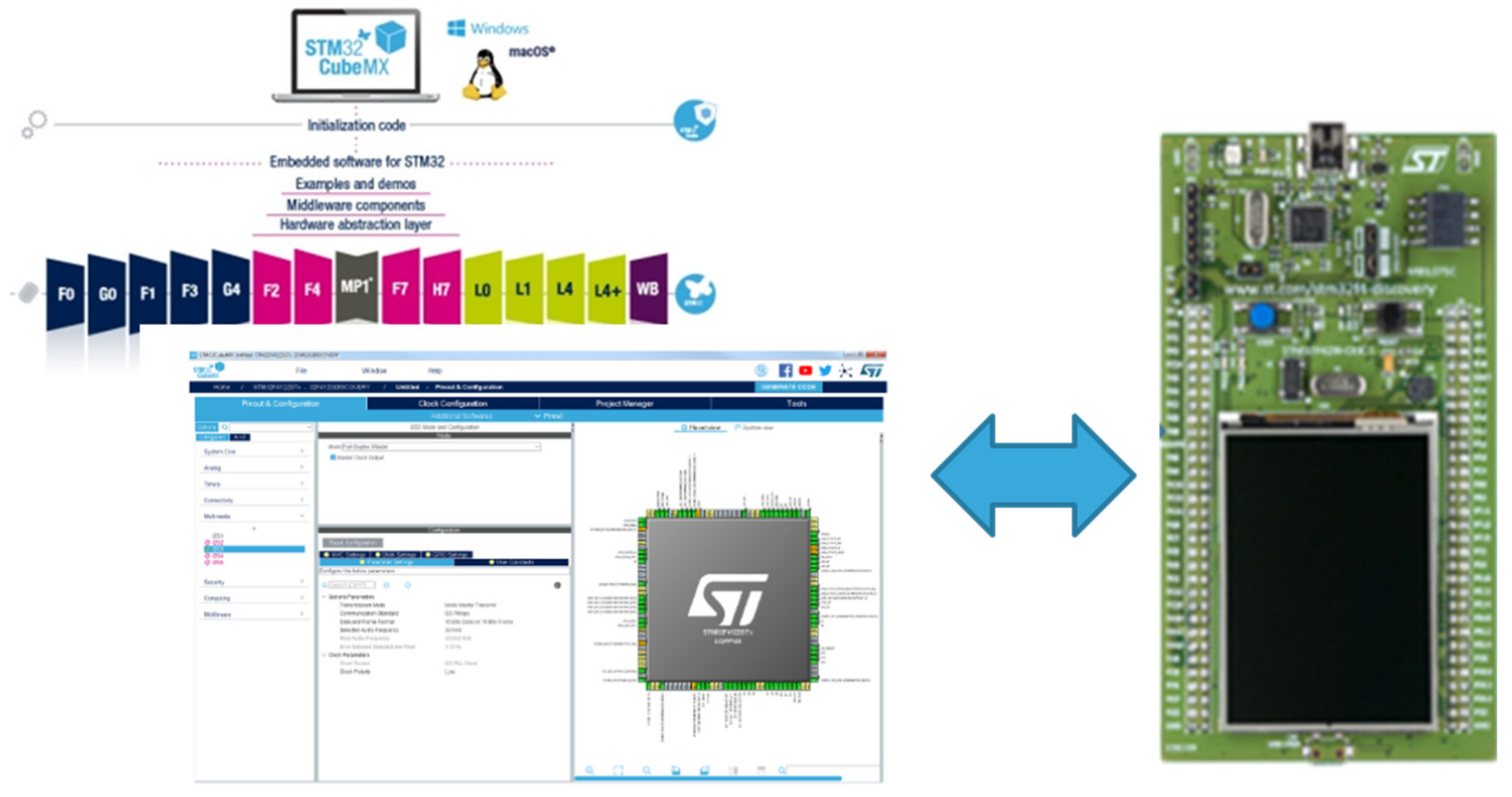
For the proposed algorithm, porting is underway at STM32 (with embedded several Cortex Ax) architectures equipped with an environment suitable for the implementation of both LSTM architectures and the RL framework [34]. The embedded system to be developed can be used by financial operators to monitor at any time and in any location (financial portable system) both the financial quotes and the forecasted trend of each financial instrument, thus being able to carry out trading operations in a mobile environment. Figure 11 shows an instance of the embedded STM32 hardware and software environment on which the proposed algorithm is being ported.
In future works, the author will propose a pipeline that—through the use of deep learning methodologies—will be able to structure financial portfolios composed of different instruments such as currencies, shares, bonds, and options; and on which an RL agent will dynamically determine the exact allocation in order to minimize risks and optimize earnings.
Author Contributions
Conceptualization, methodology, software, validation, formal analysis, investigation, resources, data curation, writing—original draft preparation, writing—review and editing, visualization, supervision, project administration, and funding acquisition, F.R.
Funding
This research received no external funding.
Conflicts of Interest
The authors declare no conflict of interest.
References
- Rundo, F.; Trenta, F.; Di Stallo, A.L.; Battiato, S. Advanced Markov-Based Machine Learning Framework for Making Adaptive Trading System. Computation 2019, 7, 4. [Google Scholar] [CrossRef]
- Rundo, F.; Trenta, F.; di Stallo, A.L.; Battiato, S. Grid Trading System Robot (GTSbot): A Novel Mathematical Algorithm for Trading FX Market. Appl. Sci. 2019, 9, 1796. [Google Scholar] [CrossRef]
- Nti, I.K.; Adekoya, A.F.; Weyori, B.A. A systematic review of fundamental and technical analysis of stock market predictions. Artif. Intell. Rev. 2019, 1–5. [Google Scholar] [CrossRef]
- Vlasenko, A.; Vlasenko, N.; Vynokurova, O.; Bodyanskiy, Y.; Peleshko, D. A Novel Ensemble Neuro-Fuzzy Model for Financial Time Series Forecasting. Data 2019, 4, 126. [Google Scholar] [CrossRef]
- García, F.; Guijarro, F.; Oliver, J.; Tamošiūnienė, R. Hybrid fuzzy neural network to predict price direction in the German DAX-30 index. Technol. Econ. Dev. Econ. 2018, 24, 2161–2178. [Google Scholar] [CrossRef]
- Li, Y.; Zheng, W.; Zheng, Z. Deep Robust Reinforcement Learning for Practical Algorithmic Trading. IEEE Access 2019, 7, 108014–108022. [Google Scholar] [CrossRef]
- Si, W.; Li, J.; Ding, P.; Rao, R. A Multi-objective Deep Reinforcement Learning Approach for Stock Index Future’s Intraday Trading. In Proceedings of the 2017 10th International Symposium on Computational Intelligence and Design (ISCID), Hangzhou, China, 9–10 December 2017; pp. 431–436. [Google Scholar]
- Chen, T.; Su, W. Local Energy Trading Behavior Modeling With Deep Reinforcement Learning. IEEE Access 2018, 6, 62806–62814. [Google Scholar] [CrossRef]
- Kumar, P.H.; Patil, S.B. Forecasting volatility trend of INR USD currency pair with deep learning LSTM techniques. In Proceedings of the 3rd International Conference on Computational Systems and Information Technology for Sustainable Solutions (CSITSS), Bengaluru, India, 20–22 December 2018; pp. 91–97. [Google Scholar]
- Ma, Y.; Han, R. Research on stock trading strategy based on deep neural network. In Proceedings of the 18th International Conference on Control, Automation and Systems (ICCAS), PyeongChang, Korea, 17–20 October 2018; pp. 92–96. [Google Scholar]
- Chen, C.T.; Chen, A.; Huang, S. Cloning Strategies from Trading Records using Agent-based Reinforcement Learning Algorithm. In Proceedings of the IEEE International Conference on Agents (ICA), Singapore, 28–31 July 2018; pp. 34–37. [Google Scholar]
- Korczak, J.; Hemes, M. Deep learning for financial time series forecasting in A-Trader system. In Proceedings of the Federated Conference on Computer Science and Information Systems (FedCSIS), Prague, Czech Republic, 3–6 September 2017; pp. 905–912. [Google Scholar]
- Wang, J.; Sun, T.; Liu, B.; Cao, Y.; Wang, D. Financial Markets Prediction with Deep Learning. In Proceedings of the 2018 17th IEEE International Conference on Machine Learning and Applications (ICMLA), Orlando, FL, USA, 17–20 December 2018; pp. 97–104. [Google Scholar]
- Lee, R.S.T. Chaotic Type-2 Transient-Fuzzy Deep Neuro-Oscillatory Network (CT2TFDNN) for Worldwide Financial Prediction. IEEE Trans. Fuzzy Syst. May 2019. [Google Scholar] [CrossRef]
- Zarkias, K.S.; Passalis, N.; Tsantekidis, A.; Tefas, A. Deep Reinforcement Learning for Financial Trading Using Price Trailing. In Proceedings of the ICASSP 2019-2019 IEEE International Conference on Acoustics, Speech and Signal Processing (ICASSP), Brighton, UK, 12–17 May 2019; pp. 3067–3071. [Google Scholar]
- Shleifer, A.; Vishny, R. The limits of arbitrage. J. Financ. 1997, 52, 35–55. [Google Scholar] [CrossRef]
- Conoci, S.; Rundo, F.; Petralta, S.; Battiato, S. Advanced skin lesion discrimination pipeline for early melanoma cancer diagnosis towards PoC devices. In Proceedings of the IEEE 2017 European Conference on Circuit Theory and Design (ECCTD), Catania, Italy, 4–6 September 2018. [Google Scholar]
- Rundo, F.; Conoci, S.; Banna, G.L.; Stanco, F.; Battiato, S. Bio-Inspired Feed-Forward System for Skin Lesion Analysis, Screening and Follow-Up. In Image Analysis and Processing - ICIAP 2017; ICIAP 2017. Lecture Notes in Computer Science; Springer: Cham, Switzerland, 2017; Volume 10485, pp. 399–409. [Google Scholar]
- Rundo, F.; Conoci, S.; Banna, G.L.; Ortis, A.; Stanco, F.; Battiato, S. Evaluation of Levenberg–Marquardt neural networks and stacked autoencoders clustering for skin lesion analysis, screening and follow-up. IET Comput. Vis. 2018, 12, 957–962. [Google Scholar] [CrossRef]
- Ortis, A.; Rundo, F.; Di Giore, G.; Battiato, S. Adaptive Compression of Stereoscopic Images. In Image Analysis and Processing – ICIAP 2013; ICIAP 2013. Lecture Notes in Computer Science; Springer: Berlin/Heidelberg, Germany, 2013; Volume 8156, pp. 391–399. [Google Scholar]
- Banna, G.L.; Camerini, A.; Bronte, G.; Anile, G.; Addeo, A.; Rundo, F.; Zanghi, G.; Lal, R.; Libra, M. Oral metronomic vinorelbine in advanced non-small cell lung cancer patients unfit for chemotherapy. Anticancer Res. 2018, 38, 3689–3697. [Google Scholar] [CrossRef] [PubMed]
- Gers, F.; Schmidhuber, E. LSTM recurrent networks learn simple context-free and context-sensitive languages. IEEE Trans. Neural Netw. 2001, 12, 1333–1340. [Google Scholar] [CrossRef] [PubMed]
- Gers, F.; Schraudolph, N.; Schmidhuber, J. Learning precise timing with LSTM recurrent networks. J. Mach. Learn. Res. 2002, 3, 115–143. [Google Scholar]
- Hochreiter, S.; Schmidhuber, J. Long short-term memory. Neural Comput. 1997, 9, 1735–1780. [Google Scholar] [CrossRef] [PubMed]
- Jithesh, V.; Sagayaraj, M.J.; Srinivasa, K.G. LSTM recurrent neural networks for high resolution range profile based radar target classification. In Proceedings of the 3rd International Conference on Computational Intelligence & Communication Technology (CICT), Ghaziabad, India, 9–10 February 2017; pp. 1–6. [Google Scholar]
- Balouji, E.; Gu, I.Y.H.; Bollen, M.H.J.; Bagheri, A.; Nazari, M. A LSTM-based deep learning method with application to voltage dip classification. In Proceedings of the 18th International Conference on Harmonics and Quality of Power (ICHQP), Ljubljana, Slovenia, 13–16 May 2018; pp. 1–5. [Google Scholar]
- Rundo, F.; Petralia, S.; Fallica, G.; Conoci, S. A nonlinear pattern recognition pipeline for PPG/ECG medical assessments. In CNS Sensors, Lecture Notes in Electrical Engineering; Springer: Cham, Switzerland, 2018; Volume 539, pp. 473–480. [Google Scholar]
- Rundo, F.; Ortis, A.; Battiato, S.; Conoci, S. Advanced Bio-Inspired System for Noninvasive Cuff-Less Blood Pressure Estimation from Physiological Signal Analysis. Computation 2018, 6, 46. [Google Scholar] [CrossRef]
- Mazzillo, M.; Maddiona, L.; Rundo, F.; Sciuto, A.; Libertino, S.; Lombardo, S.; Fallica, G. Characterization of sipms with nir long-pass interferential and plastic filters. IEEE Photon. J. 2018, 10, 1–12. [Google Scholar] [CrossRef]
- Vinciguerra, V.; Ambra, E.; Maddiona, L.; Romeo, M.; Mazzillo, M.; Rundo, F.; Fallica, G.; Di Pompeo, F.; Chiarelli, A.M.; Zappasodi, F.; et al. PPG/ECG multisite combo system based on SiPM technology. In CNS Sensors, Lecture Notes in Electrical Engineering; Springer: Cham, Switzerland, 2018; Volume 539, pp. 353–360. [Google Scholar]
- Rundo, F.; Banna, G.L.; Conoci, S. Bio-Inspired Deep-CNN Pipeline for Skin Cancer Early Diagnosis. Computation 2019, 7, 44. [Google Scholar] [CrossRef]
- Battiato, S.; Rundo, F.; Stanco, F. Self Organizing Motor Maps for Color-Mapped Image Re-Indexing. IEEE Trans. Image Process. 2007, 16, 2905–2915. [Google Scholar] [CrossRef] [PubMed]
- Tickstory—Historical Data & Resources for Traders. Available online: https://tickstory.com/ (accessed on 12 September 2019).
- STM32 Platform. Available online: https://www.st.com/content/st_com/en/about/innovation---technology/artificial-intelligence.html (accessed on 12 September 2019).
Figure 1.
(a) The EUR/USD and GBP/USD close price time-series at 1M timeframe (year: 2018). The strong correlation between the two financial series is evident from the figure reported in (b).
Figure 1.
(a) The EUR/USD and GBP/USD close price time-series at 1M timeframe (year: 2018). The strong correlation between the two financial series is evident from the figure reported in (b).
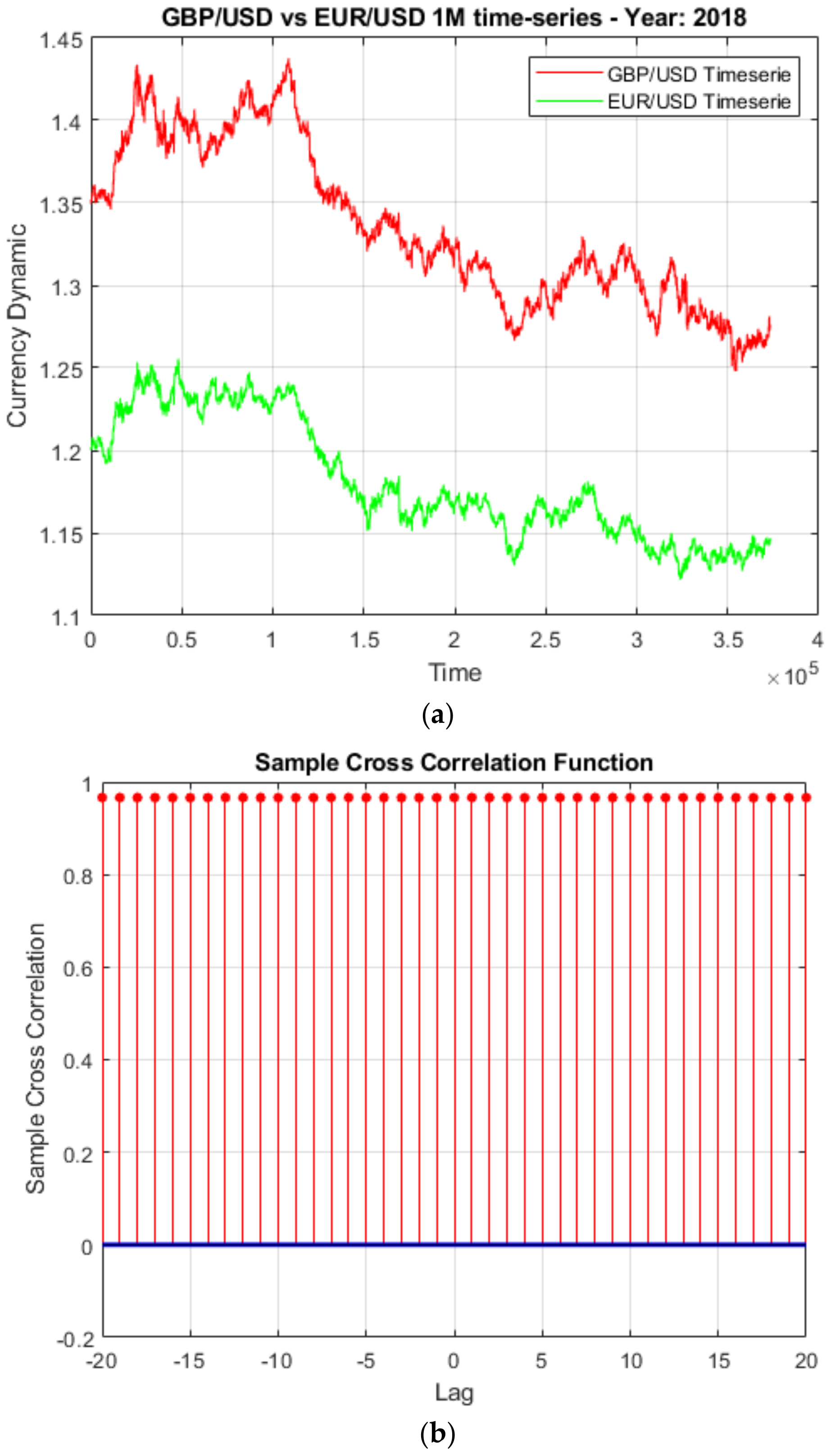
Figure 2.
Proposed currency trend forecast pipeline.

Figure 3.
The normalized EUR/USD, GBP/USD, EUR/GBP close price time-series (for year 2018).

Figure 4.
Deep LSTM model with a detail about the cell unit.

Figure 5.
Classical LSTM cell diagram.

Figure 6.
The proposed LSTM based mid-term trend prediction. The input currency time-series is being fed into LSTM input at blocks of close price quotations with a length of 100 (blue/green/red part of the input financial time-series). The output of the deep framework is a trend prediction (0: SHORT; 1: LONG; 2: Trading Range) related to next 100 close price quotations of the EUR/USD.
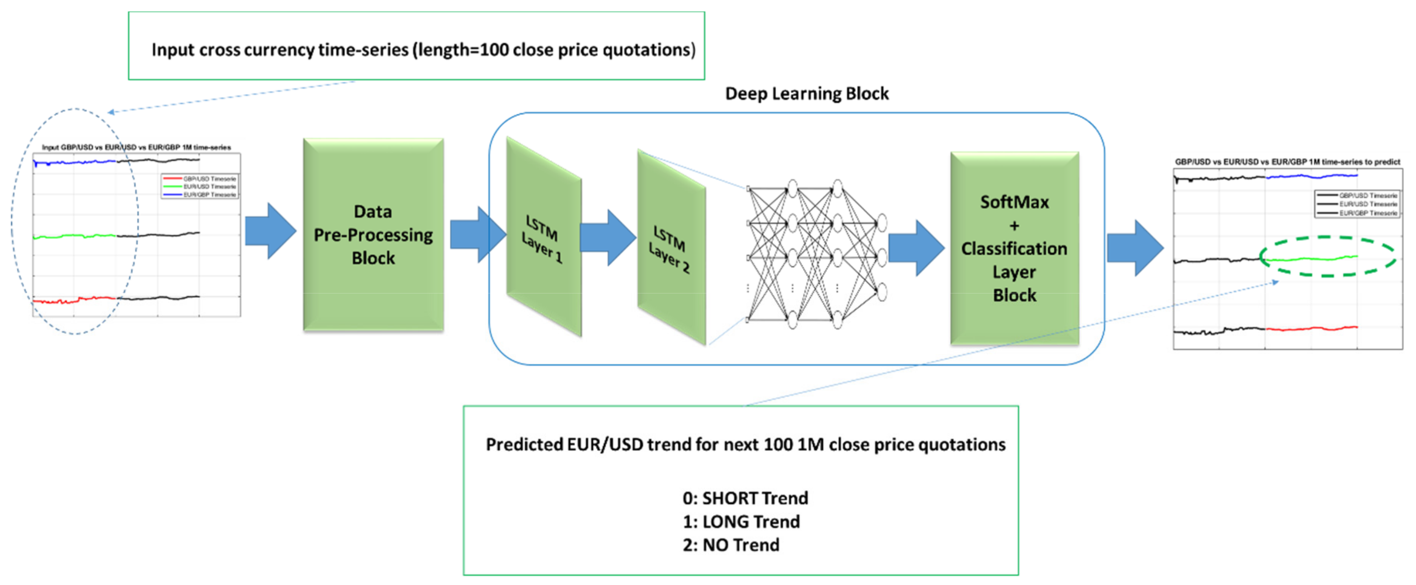
Figure 7.
Learning/validation accuracy of the previous deep learning block.
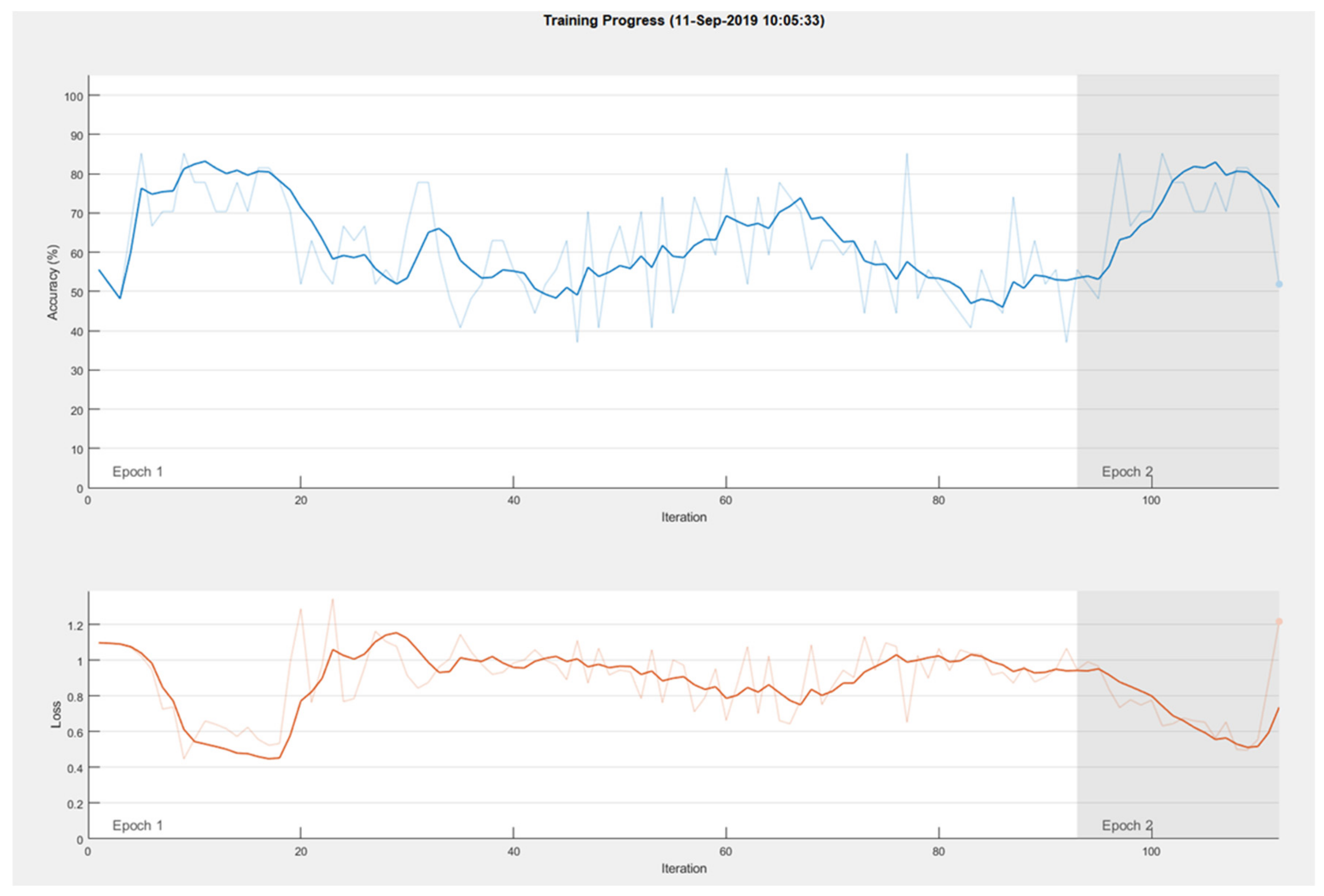
Figure 8.
Proposed reinforcement learning block to correct the predicted trend made by the deep learning block.
Figure 8.
Proposed reinforcement learning block to correct the predicted trend made by the deep learning block.

Figure 9.
The reward dynamic—during the learning phase—of the defined RL motor map system to correct the trend prediction made by previous deep learning block.
Figure 9.
The reward dynamic—during the learning phase—of the defined RL motor map system to correct the trend prediction made by previous deep learning block.
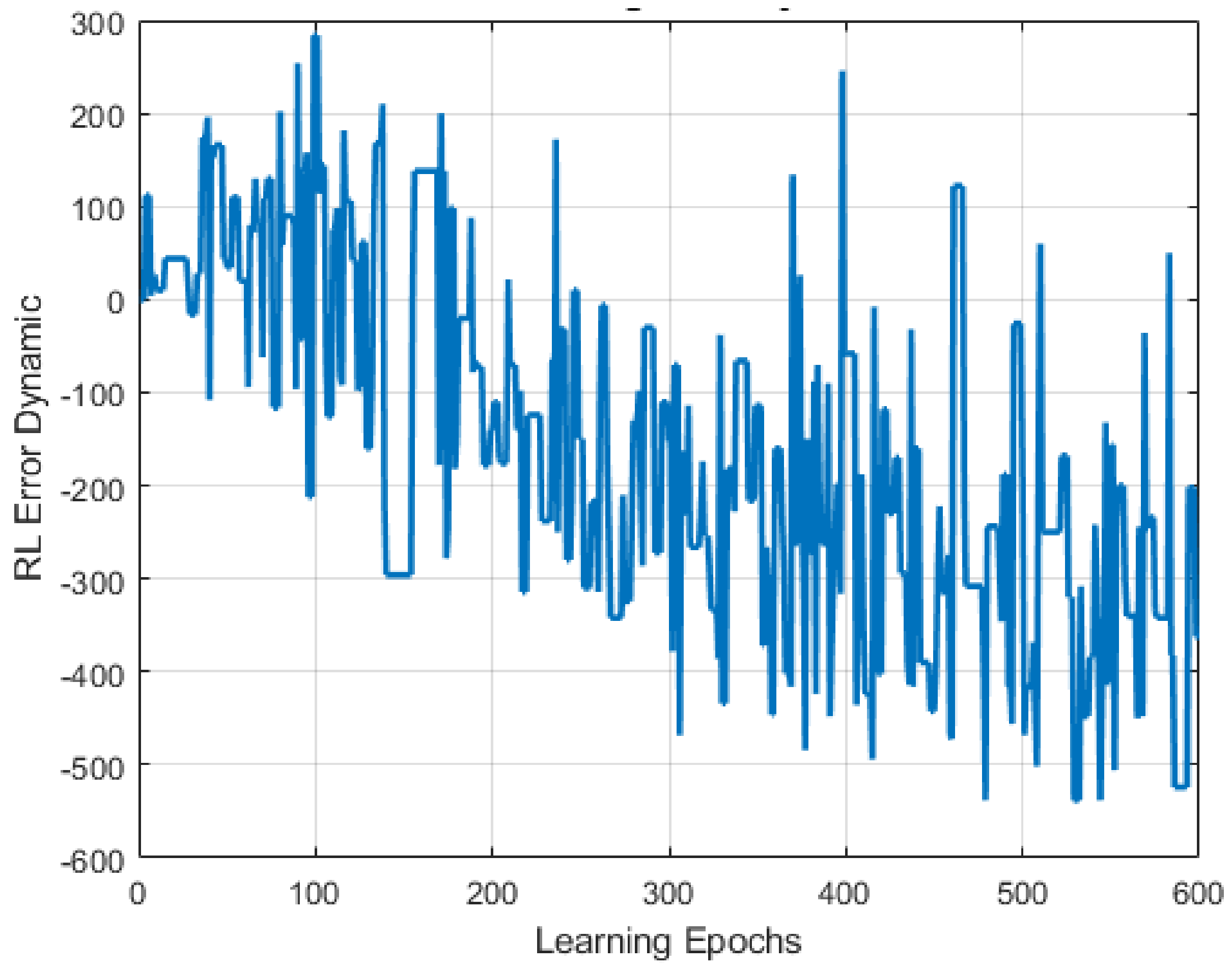
Figure 10.
GUI interface of the proposed trading system pipeline.

Figure 11.
The STM32 embedded platform for hosting the proposed pipeline as firmware.

Table 1.
Trend forecast performance accuracy for \EUR/USD currency
| Financial Year | Deep Learning Prediction Block | Deep Learning Prediction Block + RL Trend Correction |
|---|---|---|
| 2015 | 71.11 % | 85.24 % |
| 2016 | 69.25 % | 83.29 % |
| 2017 | 73.98 % | 87.16 % |
| 2018 | 70.23 % | 84.92 % |
Table 2.
Trading performance analysis of the proposed pipeline.
| Method | FX Currency Cross | ROI (%) | MD (%) |
|---|---|---|---|
| Grid Trading System [2] | EUR/USD | 94.11 | 11.25 |
| Trading System [31] | EUR/USD | 60.77 | 21 |
| Threshold (0.03%)—Strategy 2 [32] | EUR/USD | 97.687 | 50.47 |
| Threshold (0.07%)—Strategy 2 [32] | EUR/USD | 62.707 | 9.93 |
| Proposed | EUR/USD | 98.23 | 15.97 |
Table 3.
Trading performance analysis of the proposed pipeline: dynamic ROI/MD.
| Year(s) | FX Currency Cross | ROI Min (%) | MD Min (%) | ROI Max (%) | MD Max (%) |
|---|---|---|---|---|---|
| 2004–2018 | EUR/USD | 97.65 | 12.66 | 98.81 | 19.28 |
© 2019 by the author. Licensee MDPI, Basel, Switzerland. This article is an open access article distributed under the terms and conditions of the Creative Commons Attribution (CC BY) license (http://creativecommons.org/licenses/by/4.0/).
Share and Cite
MDPI and ACS Style
Rundo, F. Deep LSTM with Reinforcement Learning Layer for Financial Trend Prediction in FX High Frequency Trading Systems. Appl. Sci. 2019, 9, 4460. https://doi.org/10.3390/app9204460
AMA Style
Rundo F. Deep LSTM with Reinforcement Learning Layer for Financial Trend Prediction in FX High Frequency Trading Systems. Applied Sciences. 2019; 9(20):4460. https://doi.org/10.3390/app9204460
Chicago/Turabian StyleRundo, Francesco. 2019. "Deep LSTM with Reinforcement Learning Layer for Financial Trend Prediction in FX High Frequency Trading Systems" Applied Sciences 9, no. 20: 4460. https://doi.org/10.3390/app9204460
Note that from the first issue of 2016, this journal uses article numbers instead of page numbers. See further details here.