3.4.1. Overview
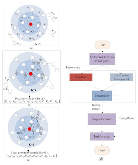
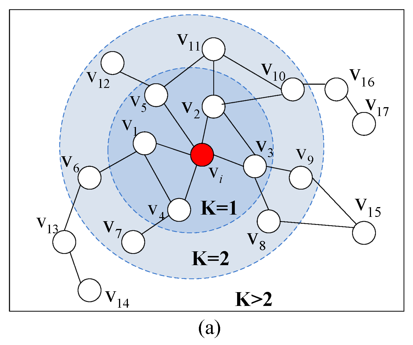
The proximity sampling strategy
S refers to sampling the network packets in the proximity of the source network packet
by random walk. We have numbered each network packet. Therefore, the result of sampling by the proximity sampling strategy
S is a list
of network packet numbers obtained by random walk. The local proximity sampling list
of a source network packet
use the strategy
S to sample high-similarity packets within the low-order proximity of
. Therefore, we want to perform random walks only within the range of low-order proximity of the source network packet
, as shown in
of
Figure 1. However, the existing graph representation learning algorithm has no ability to control the random walk range, which makes it easy to random walk to a high-order proximity farther away from the source network packet
. The random walk of the existing graph representation learning algorithm is shown in
of
Figure 1. Therefore, existing algorithms suffer from inaccurate local proximity sampling list
of source network packet
. In detail, the result of the local proximity sampling list
of
is the basic of the local proximity features of
. Therefore, the local proximity features obtained by existing preprocessing algorithms does not have the ability to accurately describe the similarity relationship between network packets.
In order to control the random walk range of node2vec within the k-order proximity, we introduced Astar to increase the penalty constraint on the random walk of node2vec. The algorithm uses the penalty term to constrain the proximity sampling range of the source network packet to ensure that the random walk is within the k-order proximity, where k is a positive integer and k can be customized. In this paper, the value of k is 2. That is to say, the random walk range of the source network packet is within the low-order proximity. Accordingly, the proposed algorithm that uses Astar to increase the penalty constraint on the random walk range of node2vec is called the packet2vec learning algorithm. In detail, the target of the packet2vec learning algorithm is that each network packet is mapped to the feature , where d is the dimension of the features obtained by the mapping, and f is a mapping function. Therefore, we find the mapping function f to map each network packet to obtain d-dimensional features. As a preliminary step of the packet2vec learning algorithm, the relational graph on packets similarity is constructed. Each network packet is treated as a node. Two basic steps of the packet2vec learning algorithm are as follows.
First of all, using the proximity sampling strategy
S to simulate a random walk process with a length
l in the neighbor of
to obtain a local proximity sample list
. The specific process to obtain the local proximity sampling list
of the source network packet
is as follows. (1) The source network packet is
, and then the proximity sampling strategy
S is used to perform penalty-based random walk in the proximity of the source network packet; (2) At each step of the penalty-based random walk, the current weight is updated according to the penalty-based weight update method. The updated weight is the new transition probability
; (3) Then select a packet for next step of the penalty-based random walk, which is equivalent to simulating the Alias sampling with time complexity
according to the updated transition probability
[
10]; (4) The above steps (2) and (3) are continuously repeated until the local proximity sampling list
of length
l is obtained. The local proximity sampling list of
obtained by the above algorithm is
, also known as
walk. In detail,
, and the sampling range of penalty-based random walk is not limited to the direct neighbor, but can be sampled by the proximity sampling strategy
S within the low-order proximity of the source network packet
.
Next, we use Skip-gram [
28] to optimize the proximity sample list
to obtain continuous
d-dimension features. The specific process is as follows. We seek to optimize the following objective function, which maximizes the log-probability of observing a network proximity
for a network packet
conditioned on its feature representation, given by
f [
10]. The objective function is shown as (1). In particular, the Skip-gram [
12] aims to learn continuous feature representations for source network packet
by optimizing a proximity preserving likelihood objective. The network packet feature representations are learned by optimizing the objective function using SGD with negative sampling [
28]. Finally, we obtain a continuous
d-dimensional local proximity feature that accurately characterizes the similarity between network packets to optimize the local neighbor proximity sample list
motivated by node2vec algorithm in [
10].
Figure 4 is a flow chart of the packet2vec learning algorithm. Algorithm 2 describes in detail the algorithm flow of obtaining the local proximity feature of the source network packet by using packet2vec preprocessing. A description of several key operations involved in Algorithm 2 is as follows.
| Algorithm 2 Packet2vec learning algorithm |
Input: Relational graph on packets similarity , Walk length of proximity sampling l, Probability of returning to the previous node p, Probability of moving away from the source node q, Penalty value .
Output: Local proximity features of network packet , which is d dimensional.
- 1:
Initialize walk to Empty. - 2:
for each node do - 3:
walk = packet2vecWalk . - 4:
end for - 5:
Skip-gram optimization(walk). - 6:
return
|
3.4.2. Astar: Penalty-Based Weight Update Method
The traditional method uses BFS random walk to obtain network packets with high similarity to the source network packets. BFS can’t limit the range of random walks, and it is easy to cause random walk to high-order proximity, as shown in
Figure 1b. Therefore, a penalty-based weight update method is introduced, which is called A star. This method is equivalent to adding a penalty constraint on the BFS, so that the range of random walk is within the
k-order proximity of the source network packet. The specific process of the penalty-based weight update method is as follows. First, we calculate the penalty value
according to the empirical formula, i.e., (the pruning threshold
the mean of weights in
−
* penalty value
). In detail, we limit the random walk within the
k-order proximity of the source network packet, then
is equal to
k. This article defines the value of
to be 2 in our experimentation. The mean of the edges is the sum of the weights of all edges in the relational graph on packets similarity
divided by the total number of edges; Next, we calculate the penalty term
of the edge according to (5) at each step of the random walk; The sum of the penalty term
and the biased weight
of the edge is calculated according to (4), which is called the penalty-based weight
. Then updates the weight value of the edge in
according to the penalty-based weight
. The graph after the weight update is recorded as
. Finally, the penalty-based weights of edge below the threshold
are pruned. Therefore, this method has the ability to control the random walk range within the
k-order proximity of the source network packet. Several key operations involved in the penalty-based weight update method are described below.
Biased weight : is a biased weight, and the calculation method is as shown in (6), where
is the weight of the edge, and search bias
has the ability to roughly control the direction of random walk. The calculation method of biased weight is same with that of the transition probability from the current node to the next node in the reference [
10].
Search bias : has the ability to roughly control the direction of random walks, such as: approximate DFS, approximate BFS. This does allow us to account for the network structure and guide our search procedure to explore different types of network proximities [
10]. This paper mainly samples the local proximity of the source network packet, so the random walk of the approximate BFS is used in this paper. The calculation method of search bias
is shown in (7), where
x is the next network packet,
is the previous network packet,
is the shortest path between the nodes
and
x. Therefore, the value of
is a value in 0, 1, 2.
Figure 5 illustrates the method of search bias
roughly control the direction of random walks.
defines two parameters
p and
q to guide the direction of random walk. Intuitively, parameters
p and
q control how fast the walk explores and leaves the proximity of starting network packet
[
10].
Parameterp: The parameter
p controls the possibility of revisiting the previous network packet immediately during the random walk [
10]. This article mainly uses random walk of approximate BFS, so the value of
p is usually
.
Parameterq: The parameter q controls that random walks tend to access network packets farther away from the network packet . This article mainly uses random walk of approximate BFS, so the value of q is usually .
If the p value is too large, the random walk may often return to the previous network packet, and it is easy to fall into the local loop search; When the p value is too small or the q value is too large, the random walk is easy to sample to the high-order proximity of the source network packet. From the above analysis, it can be concluded that the random walk with only the biased weight has no ability to accurately characterize the local proximity features of the source network packet. Therefore, we use the penalty to constrain the range of random walks to obtain local proximity features that have the ability to accurately characterize the similarity of network packets.
Penalty : is the penalty for the next network packet, and the calculation method is as shown in (5), where is the shortest path length from the source network packet to the next network packet. is the penalty value, so . The role of is to increase the penalty if the next network packet is far away from the source network packet during random walk. The farther the next network packet is from the source network packet, the larger the penalty . The penalty has the ability to control the range of random walk;
Penalty-based weight : is a penalty based weight, also known as the transition probability from the current network packet to the next network packet. The penalty based weight
is calculated as shown in (4). Considering a random walk that just traversed edge
and now resides at network packet
v [
10]. When a random walk requires the selection of a network packet for the next step, the penalty-based weight
on the edge
needs to be evaluated. The penalty based weight
is the sum of the penalty
and the biased weight
, where
v is the current network packet. If the penalty term
is 0, the packet2vec leaning algorithm is the node2vec [
10] leaning algorithm.
Node2vec based on penalty constraints has the ability to obtain local proximity features of each network packet more accurately. In the local proximity representation of each network packet, a random walk is used to capture the relationship between network packets. The relational graph on packets similarity
is transformed into a set of network packet lists by random walk. The frequency of occurrence of the network packet pairs in the set measures the structural distance between the network packet pairs [
10]. In detail, the closer the network packet is, the higher the similarity of the network packet. Algorithm 3 details the weight update strategy of the similarity relationship graph.
| Algorithm 3 Penalty-based weight update for similarity relation graph (Abbreviated as PBWeight) |
Input: Relational graph on packets similarity , Probability of returning to the previous node p, Probability of moving away from the source node q, Penalty value , Current node , Shortest path length between each pair of nodes , proximity nodes of the current node , Pruning threshold .
Output: Weight after punishment , Relational graph of network packet similarity after punishment .
- 1:
Deepcopy(). - 2:
for in do - 3:
g(cur) - 4:
h(cur) - 5:
g(cur) + h(cur) - 6:
if then - 7:
Update graph according to the value of - 8:
end if - 9:
end for - 10:
return
|
3.4.3. Packet2vecwalk: Random Walk with Penalty for Packet2vec Learning Algorithm
We consider the proximity of the source network packet from the similarity relational graph as a local search problem. We propose a flexible proximity sampling strategy based on penalty for random walk, which controls the range of random walk. The proposed algorithm uses random walk similar to BFS.
Random walk: The source network packet is
, and the length of the random walk we need to simulate is
l. Our goal is to generate a local proximity sample set
of the source network packet
. Assume that random walks are started from the source network packet
, and the
network packet in the random walk is
. In detail, the network packet
is generated by the following distribution [
10].
where
is the weight based on the penalty.
is the weight between the nodes
v and
x after the update based on the penalty weight.
Z is the normalizing constant [
10].
E is a collection of edges. Algorithm 4 describes the random walk with penalty for packet2vec learning algorithm.
| Algorithm 4 Packet2vecWalk: Random walk with penalty for packet2vec learning |
Input: Relational graph on packets similarity , Start node , Penalty value , Walk length of proximity sampling l.
Output: Local proximity features of source network packet obtained by packet2vec walk.- 1:
Initialize walk to . - 2:
Dijstra(G). - 3:
for to l do - 4:
PBWeight . - 5:
GetProximities() - 6:
AliasSample() - 7:
Append s to - 8:
end for - 9:
return
|


