Abstract
In this study, the time-averaged and instantaneous slipstream velocity, time-averaged pressure, wake flows, and aerodynamic force of a high-speed train (HST) with different nose lengths are compared and analyzed using an improved delayed detached-eddy simulation (IDDES) method. Four train models were selected, with nose lengths of 4, 7, 9, and 12 m. To verify the accuracy of the numerical simulation results, they were compared with wind tunnel test results. The comparison results show that the selection of the numerical simulation method is reasonable. The research results show that with increasing nose length, the peak values of the time-averaged slipstream velocity of the trackside position (3 m from the center of track and 0.2 m from the top of rail) and the platform position (3 m from the center of track and 0.2 m from the top of rail) decrease continuously, and show a trend of rapid reduction at first, and then a slow decrease. As the nose length increased from 4 to 12 m, the time-averaged slipstream velocity at the trackside position and platform position are decreased by 57% and 19.5%, respectively. At a height of 1.6 m from the top of the rail, ΔCP max (maximum pressure coefficient), |ΔCP min| (the absolute value of minimum pressure coefficient), and ΔCP (pressure change coefficient) decrease with increasing nose length, which is similar to the peak value of time-averaged slipstream velocity, decreasing rapidly at first and then slowly. As the nose length increased from 4 to 12 m, decreases of ΔCP max, |ΔCP min|, and ΔCP by 26.5%, 58.5%, and 44.8% were shown, respectively. Different nose lengths also have a significant impact on wake flow.
1. Introduction
The aerodynamic performance of a high-speed train (HST) is closely related to its nose shape [1], such as wake flow, train surface pressure, and aerodynamic force. According to this characteristic, the aerodynamic performance of the train can be improved by optimizing the nose shape of the train, especially to reduce the aerodynamic drag force of the train, which will be beneficial to the increase of train speed and the reduction of energy consumption [2,3]. Therefore, the research on the influence of nose shape on train aerodynamic performance has attracted the attention of a large number of scholars.
With the improvement of computing power, some scholars have studied the evolution mechanism of the flow field with different nose shapes by numerical simulation and revealed the basic law of the influence of train nose shape on flow field. For example, Niu et al. [3] used the improved delayed detached-eddy simulation (IDDES) method to study the aerodynamic performance of 8 and 12 m nose trains. It was found that nose length has a great influence on train drag, lift force, development of the boundary layer, pressure, and velocity around the train, and the wake vortex. Hassan et al. [4] used the large eddy-simulation (LES) method to study the time-averaged flow and instantaneous flow of trains with different nose lengths under crosswind conditions. The results showed that the flow on the leeward side and top of the train is different with different nose lengths. Chen et al. [5] also studied the aerodynamic performance of trains with different nose lengths under crosswind conditions. It was found that the change of nose length had effects on train surface pressure, horizontal slice pressure, and vortex structure on the leeward side of the train. The vortex intensity on the leeward side and tail can be weakened by increasing the nose length of the train. Xie et al. [6] studied the pressure on the rail side of different nose shapes (bulge-wide, ellipsoid, spindle, and flat-wide types), and found that the peak value of trackside pressure caused by the bulge-wide shape was the largest.
Numerical simulation is one of the important methods used to study the influence of train nose shape on train aerodynamic performance. However, there are many factors that affect the train nose shape, and the numerical simulation of each will increase the cost of nose shape design. Therefore, some scholars have used some optimization methods to improve the efficiency of nose shape optimization. For example, Krajnović [7] and Yao et al. [8] used the response surface method (RSM); Vytla [9], Howe [10], and Muñoz-aniagua et al. [11] used the genetic algorithm (GA), and Jakubek and Wagner [12] and Muñoz-Paniagua et al. [13] utilized the adjoint method (AM). After, the numerical simulation of the optimized model is carried out with these methods, and the results of the numerical simulation are used to judge whether the optimization goal is achieved, including improving the drag, lift force, and lateral stability of the train, among other characteristics.
In addition to the numerical simulation method, some scholars have used wind tunnels to study the influence of nose shape on the aerodynamic performance of trains. Cheli et al. [14] studied the EMUV250 train model with different nose shapes by wind tunnel testing, and it was found that the lift force, lateral force, and overturning moment of the new model were reduced. Zhang and Zhou [15] used wind tunnel tests to compare the aerodynamic forces and moments of different nose shapes under different yaw angles, and the results showed that the nose shape has a significant impact on aerodynamic forces and moments. Bell et al. [16] studied the slipstream and wake flows of simplified trains with different roof slant angles by wind tunnel experiments, and it was found that the nose length had a great influence on the separation of wake vortex. Through the wind tunnel tests, it was found that because of the different nose shapes of a train, the flow-field structure around the train is different, which leads to the change in the distribution of the train surface pressure, especially the pressure distribution of the streamlined head, which, in turn, leads to differences in the aerodynamic forces and moments of the train.
At present, research on the influence of nose shape on train aerodynamic performance is conducted more to analyze the influence of train nose shape change on aerodynamic force, aerodynamic moment, train surface pressure, pressure distribution around a train, and wake vortex structure. However, few scholars have paid attention to the relationship between wake and slipstream when the nose length changes. According to previous research, in the near-wake region, the slipstream will have a large peak value, which is due to the wake of twin counter-rotating vortices continuing to develop outward and downward beyond the width of the train. It is under this condition that the largest slipstream velocities are measured [15,17,18]. In addition, when the train passes, for static people and objects along the railway, a gust will be produced accompanied by pressure and velocity transients [19,20]. As a result, by studying the relationship between the wake and slipstream under different nose lengths, it contributes to design the train nose shape and reduce the harm to static people and objects around the train.
The main purpose of this study was to study the flow-field structure around a HST with different nose lengths, including the time-averaged and instantaneous slipstream velocity and the time-averaged pressure and wake flows. Furthermore, the aerodynamic drag and lift force of the head and tail of a train with different nose lengths will be compared and analyzed. Finally, the basic laws of aerodynamic performance with different nose lengths are obtained. Four nose lengths are used in this study: 4, 7, 9, and 12 m. The research structure of this study is divided into the following five sections: Section 2 covers methodology, including model geometry, computational domain, boundary conditions, numerical method, mesh strategy, and mesh sensitivity. The algorithm validation is presented in Section 3. Qualitative and quantitative results are given in Section 4. Conclusions are summarized in Section 5.
2. Methodology
2.1. Model Geometry
In this study, a 1:8 scale HST model is used for numerical simulation, as shown in Figure 1. The width (W) and height (H) of the train are 0.423 and 0.4825 m, respectively, and the cross-sectional area is 0.175 m2. The height H is the characteristic length in this study. The train model consists of three cars, that is, the head car, middle car, and tail car, with bogies and inter-carriage gaps, as shown in Figure 1c. The lengths of the head and tail cars are 6.59H, the length of the middle car is 6.35H, and the total length is 19.79H. Four nose lengths, namely 4, 7, 9, and 12 m, are selected, as shown in Figure 1b. To study the impact of nose length on the aerodynamic performance of the train, the streamlined length of the train is changed, the nose height of the four model trains is kept consistent, the position of the bottom bogie is the same, and the total length of the three trains is also the same.
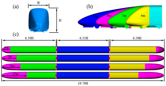
Figure 1.
Train model. (a) Height and width, (b) different nose lengths, (c) top view.
2.2. Computational Domain and Boundary Conditions
The calculation domain and boundary conditions of the numerical simulation in this study are shown in Figure 2. The length, width, and height of the calculation domain are 76.62 H, 31.05 H, and 12.95 H, respectively. The distance from the side to the y-axis symmetry plane of the calculation domain is 15.54 H. The distance from the calculation field entrance to the tip of the nose is 15.54 H. To ensure the full development of the wake flow, the nose tip of the tail car is farther away from the exit of the calculation domain, which is 42.39 H.

Figure 2.
Computational domain and boundary conditions.
The initial boundary conditions of the calculation domain must be given before the numerical simulation calculation. The side and top faces of the computational domain are symmetric boundary conditions. The train surface is a fixed boundary condition. A uniform free-stream velocity of U∞ = 60 m/s is set at the inlet. The outlet is the pressure outlet, and the boundary value P∞ = 0 Pa. The ground is moving no-slip wall boundary condition, the speed is the same as the train speed, and the direction is opposite. The Reynolds number (Re) is 1.97 × 10⁶, based on the height of the train, H, and the train speed, utrain.
2.3. Numerical Method
At present, numerous scholars have used the IDDES (based on the k-ω shear-stress transport turbulence model) method to study the unsteady aerodynamic performance around a train. For example, Wang et al. [21] compared the accuracy of different turbulence models in predicting the slipstream. The results show that the slipstream velocity obtained with the IDDES method has good consistency with experimental data. Wang et al. [22] used the IDDES method to study the influence of ground conditions on the slipstream velocity of a HST. Xia et al. [23] studied the effects of ground configurations on the aerodynamic performance of the HST using the IDDES method. Niu et al. [3] and Chen et al. [12] studied the effects of train nose length on aerodynamic performance by the IDDES method. This paper also uses the IDDES (based on k-ω shear-stress transport) method to study the flow field around a HST.
The IDDES combines the advantage of delayed detached-eddy simulation (DDES) with an improved RANS (Reynolds-averaged Navier-Stokes)-LES hybrid model aimed at wall modelling in LES (WMLES) [24]. Because the IDDES combines DDES with WMLES, the length-scale must be redefined. The IDDES length-scale is defined as:
where the RANS length-scale lRANS = κ1/2/(Cμω), the LES length-scale lLES = CDESΨΔ, the blending function, , is defined as , and fdt is the delay function defined in Spalart’s literature [25]. fB is an empirical blending-function, which varies from 0 to 1, and fe is an elevating function, which is aimed at preventing the excessive reduction of the RANS Reynolds stresses.
In addition, the new sub-grid length-scale is defined by:
and
where hwn is the grid step in the wall-normal direction and Cw is an empirical constant set as 0.15. hx, hy, and hz are the local streamwise, wall-normal, and lateral cell sizes, respectively. For more information, see Shur et al. [24].
An implicit-unsteady segregated incompressible finite-volume solver was used in this study. The convection term used hybrid second-order upwind and bounded-central differencing (hybrid-BCD) and the temporal scheme was selected as second order for this numerical simulation. Because of the Mach number (Ma = U∞/c, where the upstream velocity U∞ = 60 m/s and c is local velocity, which is equal to 340 m/s), Ma = 0.176 < 0.3 and the gas density is constant. In this study, the initial solver used steady RANS, which can make the residuals converge more easily and shorten the calculation time. For the unsteady numerical simulation calculation, the physical time step is 0.062 t* (t* = tU∞/H), and each time step is iterated 20 times and total number of time steps is 4000. The residual of each turbulence equation can be achieved 10−4 in each time step. The STAR-CCM+ of the National Supercomputing Center (Wuxi, China) was used for calculation. There are altogether six cases in this calculation, with each case calculated by eight nodes.
2.4. Grid Strategy
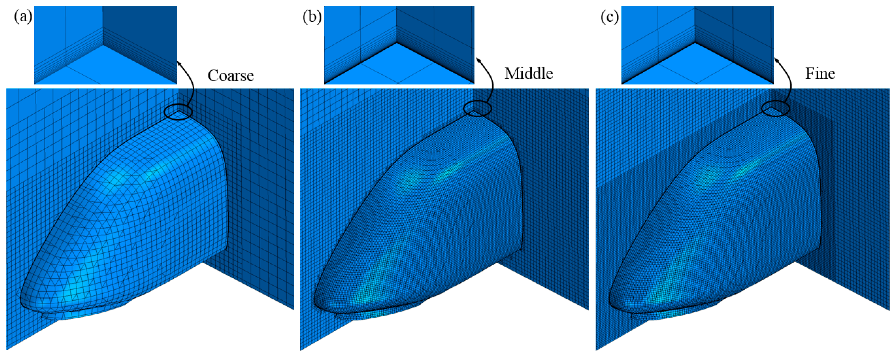
Grid generation adopts the CD-adapco grid-generation technology in STAR-CCM+. The grid of the computational domain uses a hybrid grid. To simulate the boundary-layer effect, the prism-layer grid is used near the train surface, and the other part of the computational domain uses a hexahedral grid. Trimming technology is used to connect prism grids and hexahedral grids. To accurately simulate the flow field around the train and control the number of grids, the computational domain is meshed by layer-by-layer encryption, and the grid space around the train is therefore smaller. Three sets of grids, i.e., coarse, medium, and fine, were used to verify the independence of the grids. The number of grids comprised by the three sets is 15 million, 31 million, and 50 million, respectively. The grids with different spatial resolutions are shown in Figure 3. For the grid surface scale of the train, the grid size of the fine and medium grid trains is 0.0065 H−0.013 H, and that of the coarse grid train is 0.013 H−0.026 H. For the local refinement area around the train, the scale of the fine grid is the smallest, and the coarse mesh has the largest scale. The medium and fine grids have 20 prism-layers near the train surface, and the coarse grid has only ten prism-layers.
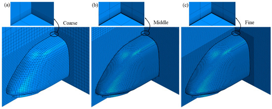
Figure 3.
Different type grids: (a) coarse, (b) middle, and (c) fine.
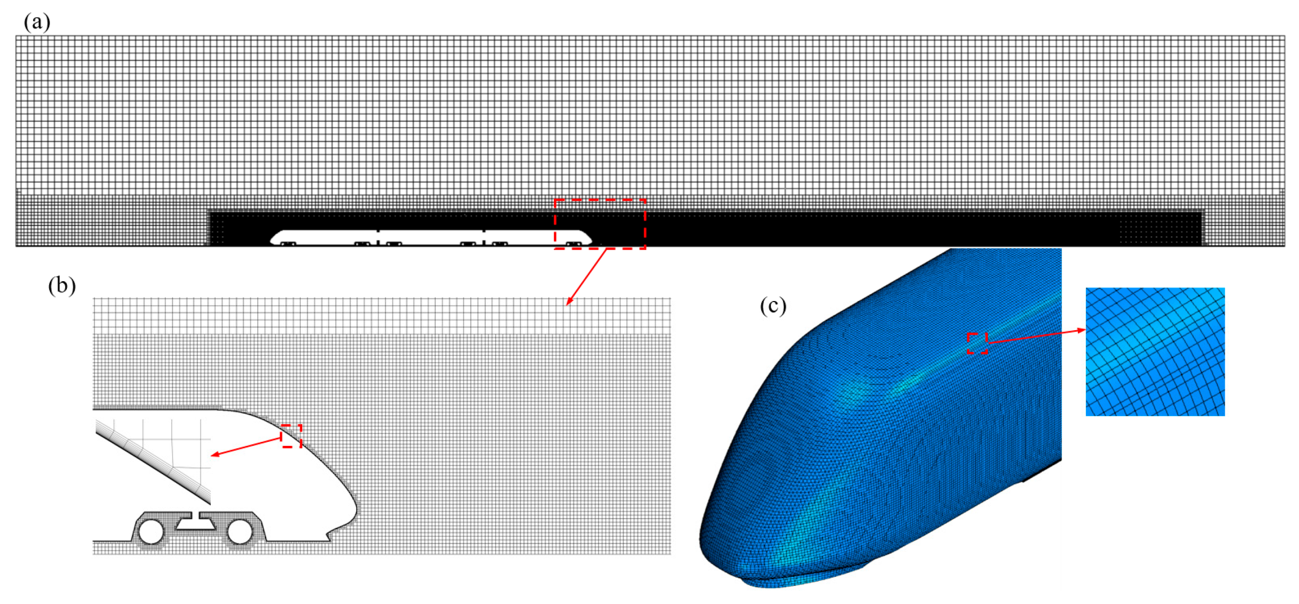
Figure 4 shows the train surface mesh, tail local refinement, and the prism-layer of the medium grid. To accurately simulate the surface of the car body and control the number of grids at the same time, the surface grid size of the bogie and the inter-carriage gaps is 0.0065 H, the surface grid size of the other parts of the car body surface is 0.013H, and there are three local refinements around the train. The Courant−Friedrichs−Lewy number (CFL = U∞Δt/Δx, where Δx is the length of cells and Δt the time step) exceeds 1 for no more than 1% of the total number of grids, and the CFL number stays below 1 for the most of grids [22,23]. A prism-layer grid generator was used to create a 20 prism-layers near the train surface with a growth rate of 1.15, with the first-layer grid having a thickness of 0.013 mm. The y+ (the non-dimensional distance to the train surface) of the train surface of the medium grid is shown in Figure 5. It can be seen from the figure that the value of y+ is approximately 1, and most areas are less than 1, except that y+ is greater than 1 on part of the surface of the streamlined part of the train and on part of the bogie. Therefore, y+ of the medium grid meets the requirements.
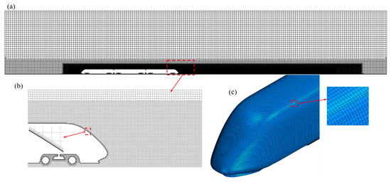
Figure 4.
Medium grid: (a) plane at y = 0, (b) prism layer, and (c) train surface.

Figure 5.
y+: (a) top view, (b) side view, and (c) bottom view.
2.5. Grid Sensitivity
The time-averaged U of the coarse, medium, and fine grids at 3 m from the center of track (COT) and 0.2 m from the top of rail (TOR) and the time-averaged pressure coefficient, Cp, at 2.5 m from the COT and 1.6 m from the TOR are shown in Figure 6, where, the time-averaged U is calculated by Equation (7), and Cp is calculated by Equation (6). The variation trend of the time-averaged U and Cp of the three sets of grids is basically the same. For the time-averaged U, the results of the medium grid are more consistent with those of the fine grid, except that the difference is larger in the boundary-layer region. For Cp, the results of the three sets of coarse, medium, and fine grids are in good agreement. Only at the peak is the value of the coarse grid slightly smaller than the values of the medium and fine grids, indicating that Cp is less sensitive to the grid than the time-averaged U. In summary, the difference between the numerical simulation results of the medium and fine grids is small, indicating that the number of grids continues to increase, and the results of numerical simulation have little effect. Therefore, the numerical simulation used in this study uses a medium grid.

Figure 6.
Mesh sensitivity: time-averaged of (a) U and (b) pressure.
2.6. Data Processing
According to EN (CEN European Standard 2010, 2013) [26,27], the drag coefficient, lift force coefficient, and pressure coefficient are defined as follows:
where Cx, Cz, and CP are drag coefficient, lift force coefficient, and time-averaged pressure coefficient, respectively. Fx and Fz are drag and lift force, respectively. The air density, ρ, is considered to be 1.225 kg/m3. The incoming flow velocity U∞, which is equal to the speed of the train, is 60 m/s. The reference area, S, was considered to be 0.175 m2. P is the local mean static pressure. P∞ is the reference pressure, which is equal 0 Pa.
3. Algorithm Validation
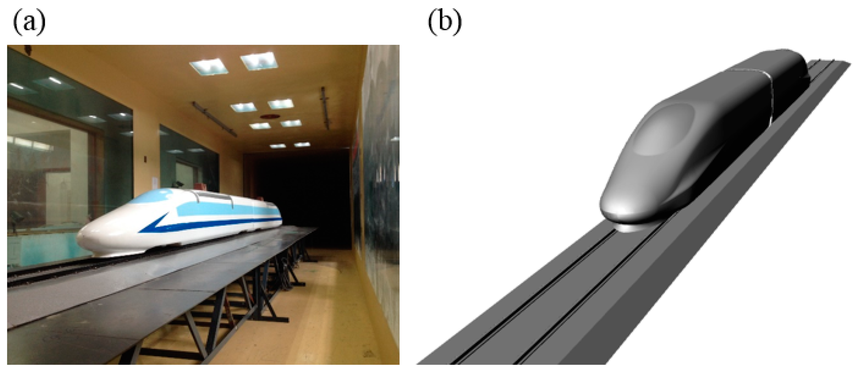
In this study, the accuracy of numerical simulation was verified by wind tunnel test results. The wind tunnel testing was carried out in the National Engineering Laboratory for High Speed Railway Construction, Central South University, China. The test model is shown in Figure 7a. Figure 7b is the computer-aided-design (CAD) model of the validation algorithm. Table 1 shows the results of numerical simulation and wind tunnel test results, as well as the differences between the two. It can be found from the table that the drag force of the head car and tail car can be in good agreement with the test results, and the error is less than 6%. However, the lift of the head car and tail car is quite different from the test results. The reason for the great difference may be that the geometric model of the train is more complex, and it is difficult to accurately simulate the small parts, such as the bottom bogie. The rough ground near the model and the installation mode of the train during the test also will affect the flow of the bottom flow field, while the bottom flow field has a great influence on the lift force [28,29,30]. Therefore, it is reasonable to conclude that this causes the difference of Cz between wind tunnel test results and numerical simulation results to be 36.41%. In conclusion, the selection of the numerical simulation algorithm in this study is reasonable.

Figure 7.
Train model: (a) wind tunnel model and (b) numerical simulation model.

Table 1.
Comparison of experimental results and numerical simulation results.
4. Results and Analysis
4.1. Aerodynamic Force Coefficient
Aerodynamic force has a great impact on the operation of a HST, in which drag force will affect the speed increase and increase energy consumption, while lift force will have an impact on the stability of train operation. In the absence of crosswind, the lateral force tends to 0. Therefore, the drag force and lift force of the head and tail cars are studied below. Cx and Cz of the head car and tail car of the train with a sample time of t* between 62 and 249 are averaged, and the time-averaged Cx and Cz of the head car and tail car with different nose lengths are obtained, respectively, as shown in Figure 8. Through comparison, it is found that Cx of the head car and tail car decrease with increasing nose length. Cz of the head car increases with increasing nose length, and Cz of the tail car first decreases and then increases with increasing nose length. When the nose length increases from 4 to 7 m, Cx and Cz change obviously, in which Cx of the head car decreases by 17.6%, Cx of the tail car decreases by 29.3%, Cz of the head car decreases by 15.8%, and Cz of the tail car decreases by 75.7%. The nose length increased from 7 to 12 m, and the difference of Cx and Cz was not obvious. It is shown that the drag coefficient and lift force coefficient can be effectively reduced by properly increasing the nose length.

Figure 8.
Time-averaged aerodynamic (a) drag coefficients, and (b) lift force coefficients of the head and tail cars.
4.2. Time-Averaged Flow
4.2.1. Time-Averaged Slipstream Velocity
A slipstream is generated because a HST will drive the surrounding air to produce a complicated flow due to the boundary-layer effect. At present, HSTs can run at speeds of more than 300 km/h, and the resulting slipstream will threaten the safety of passengers on the platform and track-side workers, and cause damage to the trackside infrastructure [17,22]. Therefore, a large number of scholars have studied the slipstream [15,17,19,21,22,23,31]. According to the Technical Specifications for Interoperability (TSI) (European Union Agency for Railways 2014) [32] and EN CEN European Standard 2009) [33], the horizontal velocity is harmful to persons and infrastructure along the line, so in this study, we mainly consider the horizontal velocity. The horizontal velocity is herein referred to as the “slipstream velocity” [17], and the dimensionless “slipstream velocity” U is defined as:
where u is the longitudinal velocity, v is the lateral velocity, and utrain is the speed of the HST.
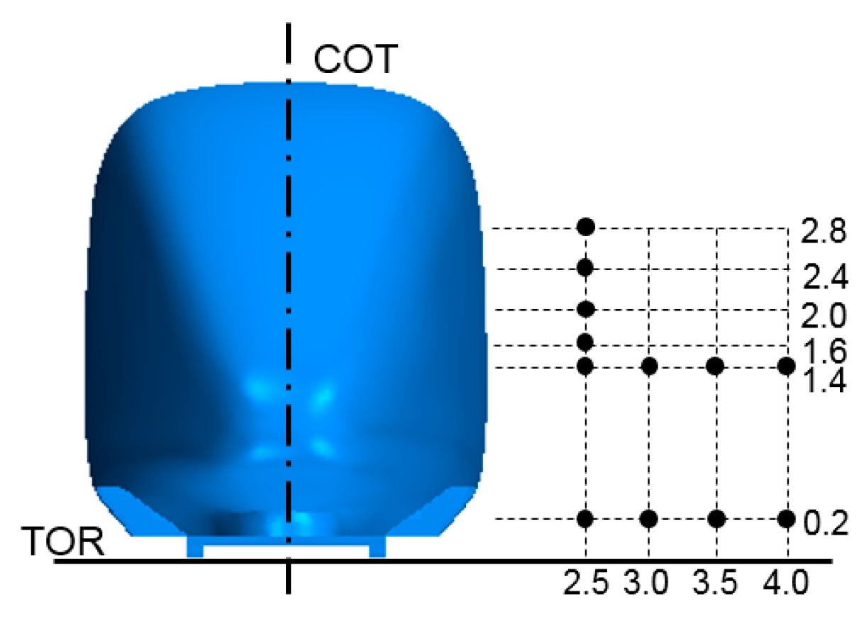
Figure 9 shows the positions of different measuring points relative to the TOR and COT, where in four points with heights of 1.6–2.8 m are the positions of the measuring points of the time-averaged pressure and the measuring points of U at heights of 0.2 and 1.4 m. At y = 3 m, z = 0.2 m and y = 3 m, z = 1.4 m, the two measurement positions are specified by the TSI (European Union Agency for Railways 2014) [32] and EN CEN European Standard 2009) [33].

Figure 9.
Position of the measurement point relative to center of track (COT) and top of rail (TOR).
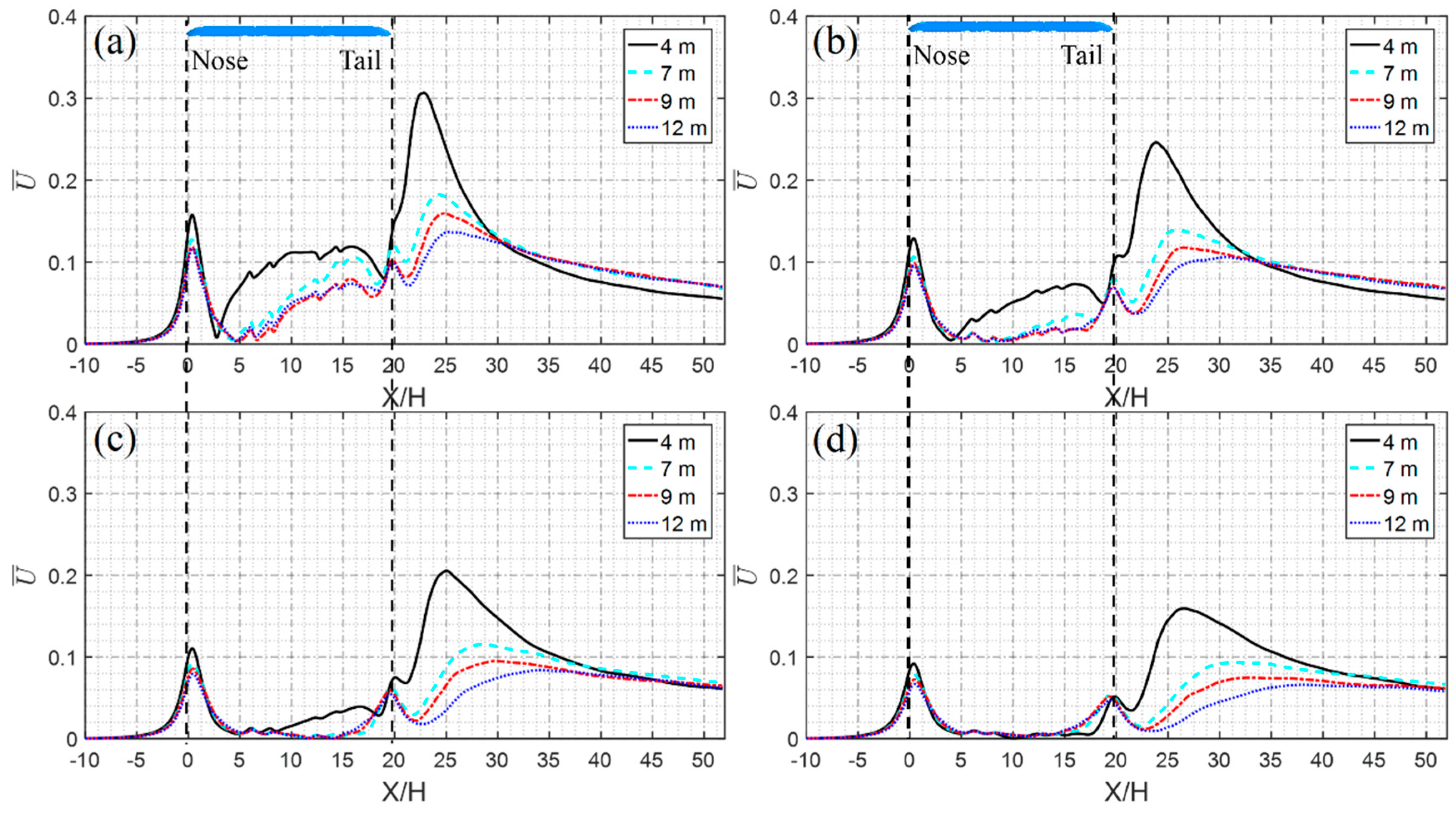
Figure 10 shows a comparison of the time-averaged U at different nose lengths at a height of z = 0.2 m from the TOR and at different positions from the COT. As can be seen from the figure, there will be a peak value of U in the nose region, and with increasing nose length, the peak value in different positions will show a decreasing trend. In the near-wake region, there also will be a larger peak. Similarly, with increasing nose length, the peak value of different positions shows a decreasing trend. In the boundary-layer region, when the nose length is 4 m, U is larger at y = 2.5, 3, and 3.5 m, while, at y = 4 m, U is basically the same with different nose lengths. At different positions from the COT, the peak value of U with a nose length of 4 m is obviously larger than that of the other lengths. When the nose length increases to 9 m, the influence on the peak value of U in the near-wake region decreases. With increasing nose length, the peak value of the wake region of U tends to move backward. When the nose length increases from 4 m to 12 m, the peak value of the near wake region decreases by 55.4% at y = 2.5 m, 57% at y = 3 m, 53.7% at y = 3.5 m, and 52.2% at y = 4 m. With increasing nose length, the effect of weakening U in the near-wake region is obvious. To study the influence of position on the peak value of U, a nose length of 4 m is taken as an example. The peak value of U is 0.307 at y = 2.5 m and 0.159 at y = 4 m, and the distance from the COT increases from 2.5 m to 4 m, decreases by 48.2%, and the value of the U decreases obviously, which indicates that the U decays faster with the increase of distance from the COT.
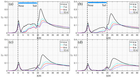
Figure 10.
Time-averaged U of different nose lengths at height z = 0.2 m from TOR for (a) y = 2.5 m, (b) y = 3 m, (c) y = 3.5 m, and (d) y = 4 m (black dashed line on left is the nose and that on right the tail).
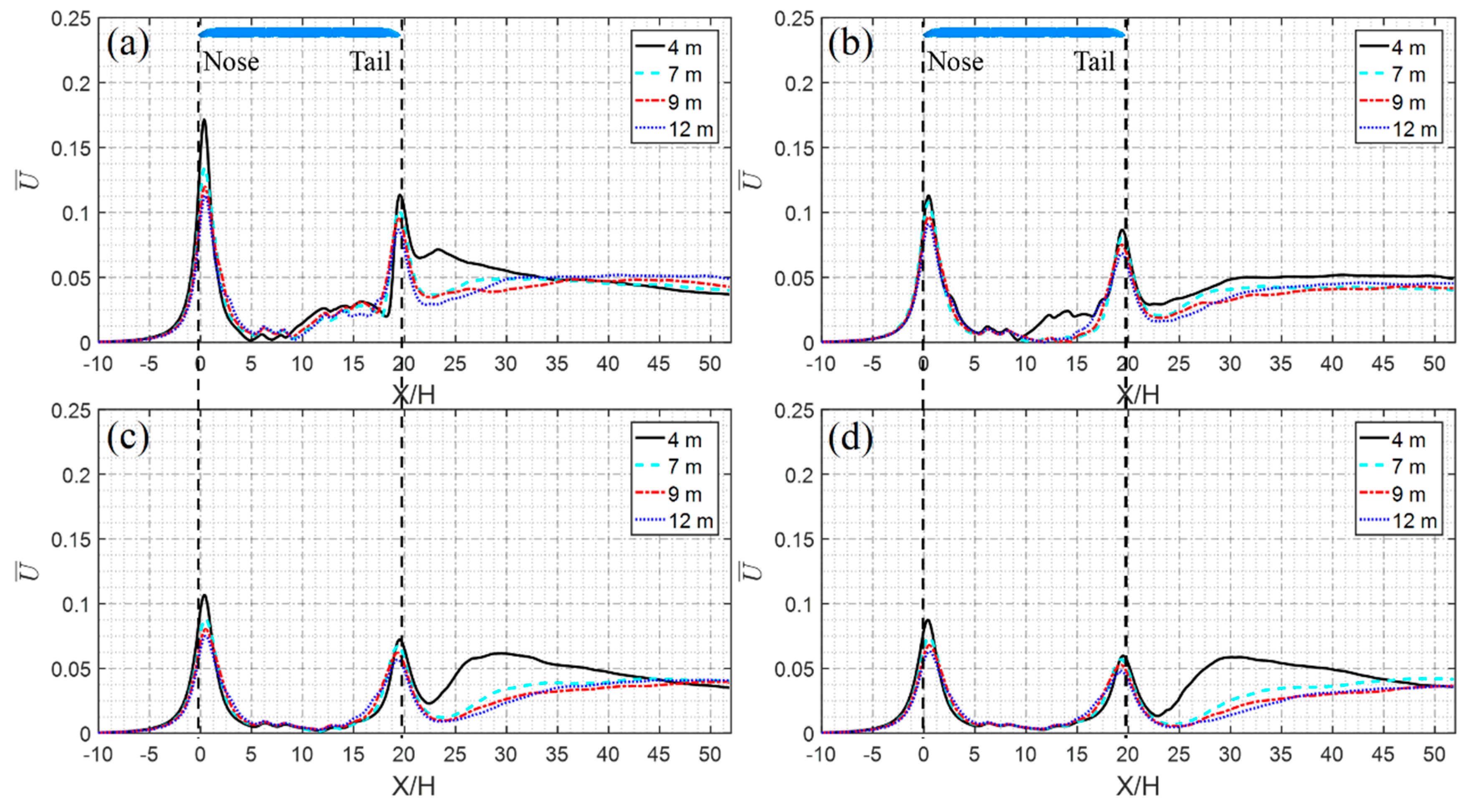
Figure 11 shows a comparison of U at different nose lengths at a height of z = 1.4 m from the TOR and at different positions from the COT. Similar to U at the trackside position, U at the platform position also peaks in the nose region and near the wake region. However, the position of the maximum peak value of U is opposite to U on the trackside position, and the maximum peak value of U at the platform position appears in the nose region. With the increasing nose length, the peak value of the nose region and the peak value of the near-wake region show a decreasing trend in different positions. When the nose length increases from 4 to 12 m, the peak value of the nose region decreases by 34.4% at y = 2.5 m, 19.5% at y = 3 m, 30% at y = 3.5 m, and 27.7% at y = 2.5 m. With increasing nose length, the attenuation of U in the platform position is slower than that in the trackside position. When the nose length is 4 m, the U peak value is 0.172 at y = 2.5 m and 0.087 at y = 4 m. The distance from the COT increases from 2.5 to 4 m, which is a 49.4% decrease. This is the same as the trackside position, i.e., the decrease is obvious, which indicates that the U attenuation at the platform position is also faster with increasing distance from the COT.
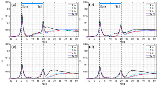
Figure 11.
Time-averaged U of different nose lengths at height z = 1.4 m from TOR for (a) y = 2.5 m, (b) y = 3 m, (c) y = 3.5 m, and (d) y = 4 m (black dashed line on left is the nose and that on right the tail).
4.2.2. Time-Averaged Pressure
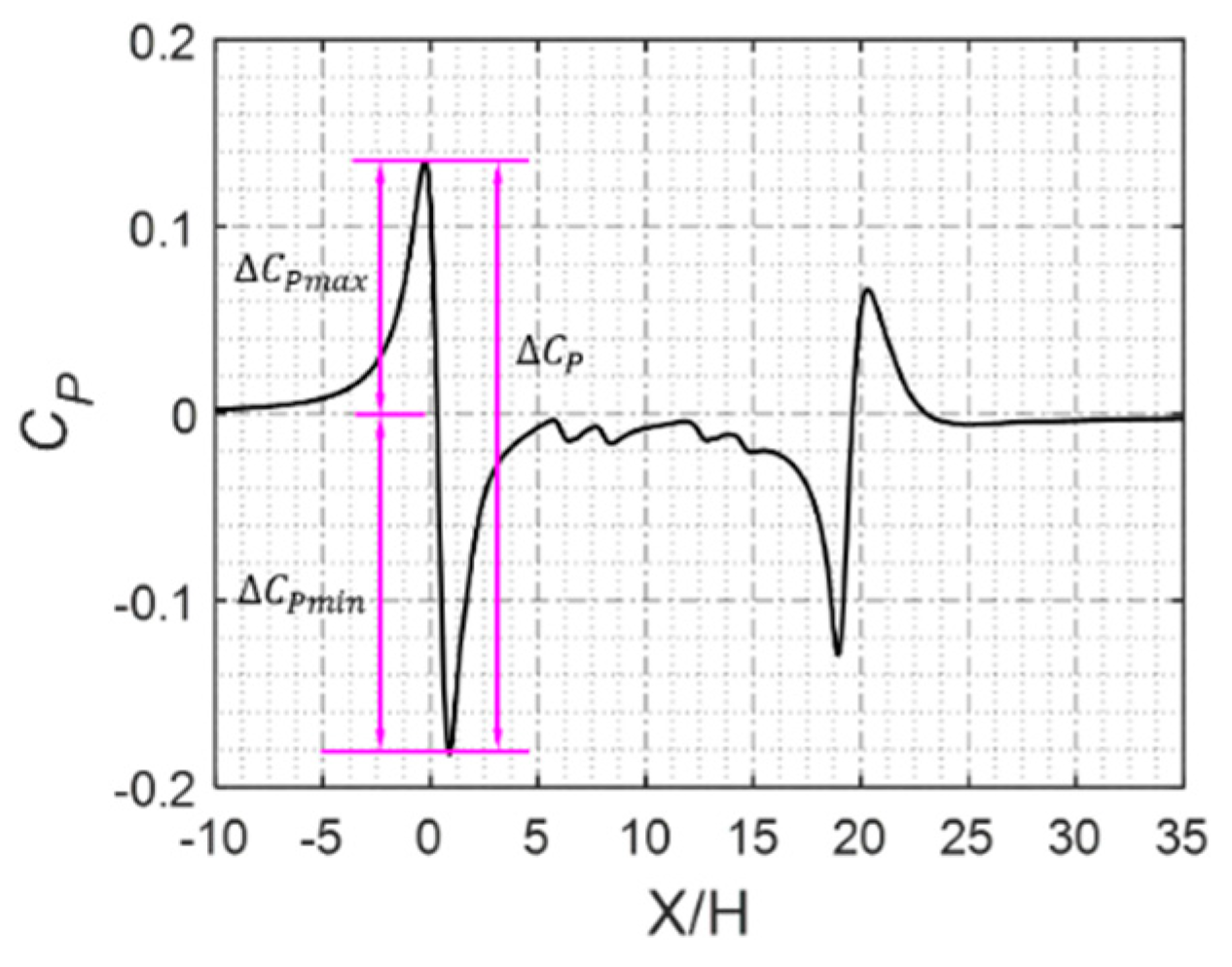
Pressure is an important criterion for evaluating the aerodynamic performance of trains. A large number of researchers have studied train pressure, including the influence of the train on the surrounding environment and the distribution of the surface pressure of the train itself. According to the TSI (European Union Agency for Railways 2014) [32] and EN 2013 (CEN European Standard 2013) [27], the position of the pressure measuring points are selected 2.5 m from the COT and the height from the top of track is 1.5–3.0 m; the position of the measuring points are shown in Figure 9. Four measuring points 2.5 m from the COT and 1.6, 2, 2.4, and 2.8 m from the TOR are selected. ΔCP max, ΔCP min, and ΔCP are defined as in Figure 12, where ΔCP max is a positive value, ΔCP min a negative peak, and ΔCP the peak-to-peak value.
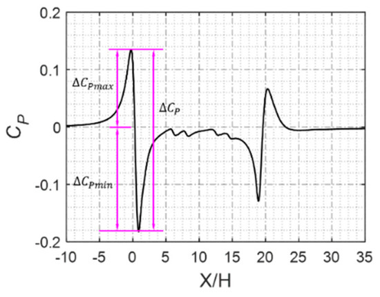
Figure 12.
Definition of maximum pressure coefficient (ΔCp max), the absolute value of minimum pressure coefficient (ΔCp min), and pressure change coefficient (ΔCp).
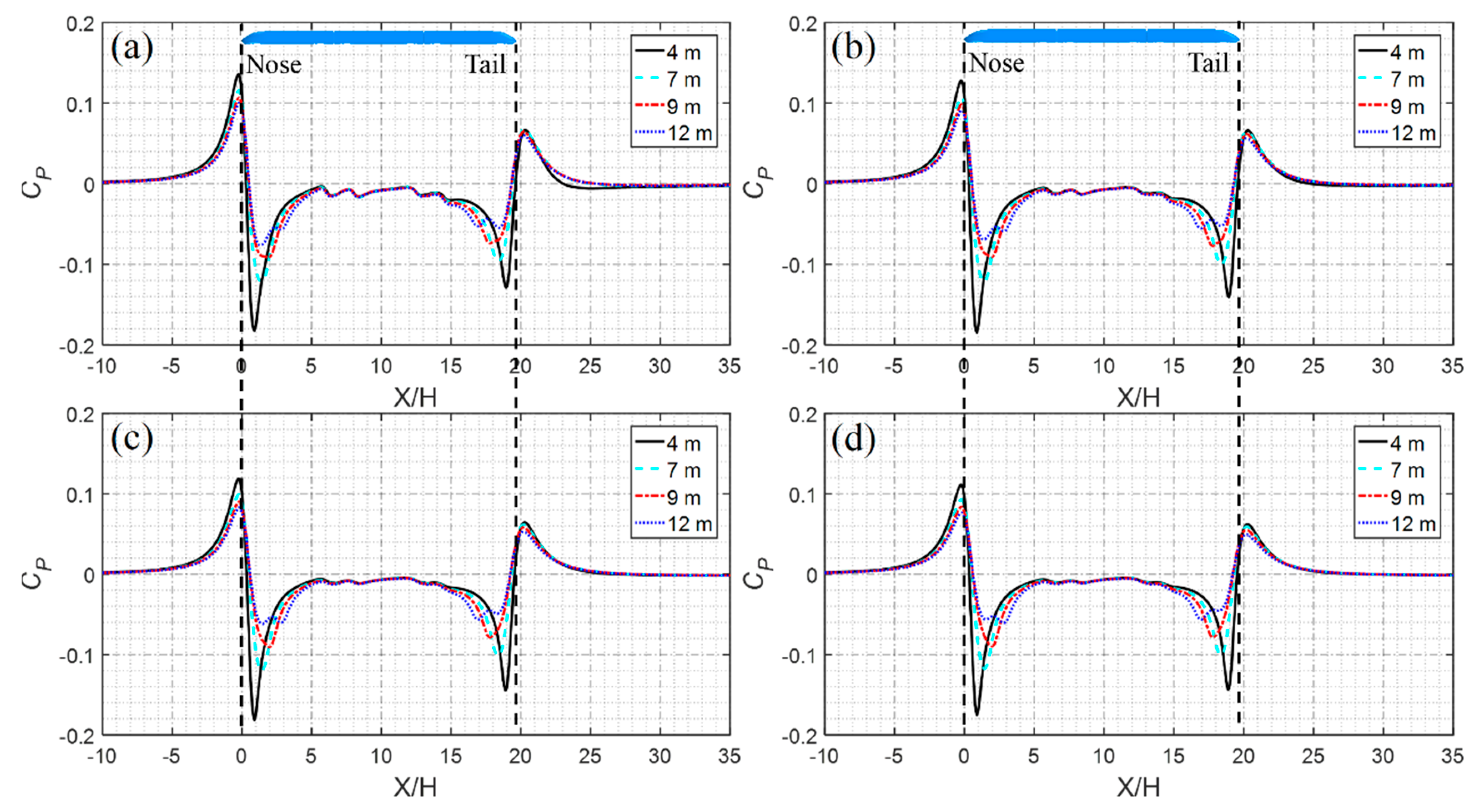
The time-averaged pressure coefficients at a distance of 2.5 m from the COT and at different heights from the TOR are shown in Figure 13. As can be seen from the figure, the pressure coefficient appears as a positive peak in the nose region, and then rapidly drops to a negative peak. There is a negative peak in the wake region, which quickly becomes a positive peak. The pressure of a HST with different nose lengths is small in the boundary-layer region, and the pressure coefficients of the train with different nose lengths have little difference in the boundary-layer region. When the nose length is 4 m, the values of ΔCP max, ΔCP min, and ΔCP are the largest, and when the nose length is 12 m, the values of ΔCP max, ΔCP min, and ΔCP are the smallest.
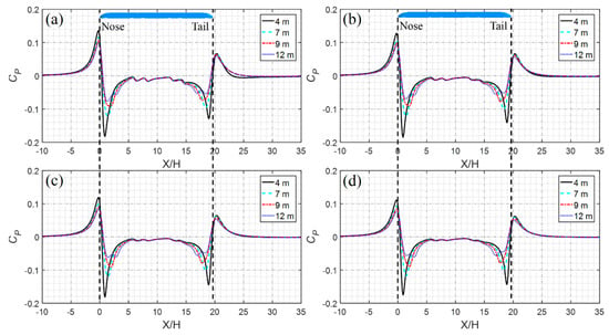
Figure 13.
Pressure coefficient at y = 2.5 m for (a) z = 1.6 m, (b) z = 2 m, (c) z = 2.4 m, and (d) z = 2.8 m (black dashed line on left is the nose and that on the right the tail).
Table 2 shows the values of ΔCP max, ΔCP min, and ΔCP at different heights with different nose lengths. It can be seen from the table that, at different heights, the values of ΔCP max, ΔCP min, and ΔCP decrease continuously with increasing nose length. At different heights, as the nose length increases from 4 to 7 m, the values of ΔCP max, ΔCP min, and ΔCP decrease faster. When the nose length increases from 7 to 9 m and from 9 to 12 m, the values of ΔCP max, ΔCP min, and ΔCP decrease slowly. At different heights, the difference between ΔCP max with nose lengths of 4 and 12 m is between 0.35 and 0.37, which indicates that the change of height has little effect on ΔCP max. At different heights, the difference in ΔCP max between nose lengths of 4 and 12 m is between 0.35 and 0.37, which indicates that the height change has little effect on ΔCP max. At z=1.6 m, the difference of |ΔCP max| and ΔCP values between nose lengths of 4 and 12 m is 0.107 and 0.143, respectively; at z = 2 m, the difference of |ΔCP max| and ΔCP values between nose lengths of 4 and 12 m is 0.116 and 0.153, respectively; at z=2.4 m, the difference of |ΔCP max| and ΔCP values between nose lengths of 4 and 12 m is 0.12 and 0.141, respectively; at z = 2.8 m, the difference of |ΔCP max| and ΔCP values between nose lengths of 4 and 12 m is 0.115 and 0.15, respectively. The difference of |ΔCP min| for nose lengths of 4 and 12 m shows a trend of first increasing and then decreasing, while the difference of ΔCP has no obvious change trend. When the nose length of the train is 4 m, the height increases from z = 1.6 m to z = 2.8 m, and the values of ΔCP max, |ΔCP min|, and ΔCP decrease continuously, decreasing by 18.4%, 4.4%, and 10.3%, respectively. ΔCP max, |ΔCP min|, and ΔCP at a height of 1.6 m from the TOR decreases with increasing nose length, and the nose length increases from 4 to 12 m, which decreases by 26.5%, 58.5%, and 44.8%, respectively. Properly increasing the length of the nose has an obvious effect on improving the pressure around the train.

Table 2.
ΔCp max, ΔCp min, and ΔCp at different heights with different nose lengths.
Figure 14 shows the time-averaged pressure coefficient CP on the surface at y = 0 m for trains of different nose lengths, with Figure 14a showing CP on the upper surface and Figure 14b showing CP on the lower surface. It can be seen from the figure that, with different nose lengths, the CP on the upper surface near the junction of the streamlined and non-streamlined nose of the head and tail cars is quite different, and the negative pressure amplitude of the head car is larger than that of the tail car. Taking a nose length of 4 m as an example, the negative pressure amplitude of the head car is 28.5% larger than that of the tail car. The pressure amplitude in the boundary-layer region with different nose lengths has little effect. When the nose length increases from 4 to 12 m, the negative pressure amplitude of the head car decreases by 74.1%, and the negative pressure amplitude of the tail car decreases by 71.2%. However, different nose lengths have little effect on the time-averaged pressure distribution on the lower surface, and only the local area exhibits a small difference. In summary, it can be seen that the nose length mainly has a great impact on the pressure distribution near the junction of streamlined and non-streamlined nose, and with increasing nose length the negative pressure amplitude decreases obviously.

Figure 14.
Train surface distribution of time-averaged pressure coefficient (CP) at y = 0 m: (a) top, and (b) lower surface.
4.3. Instantaneous Flow
The evaluation of the slipstream of a HST is generally based on the characteristic speed U2σ guided by the technical specification for interoperability (TSI) [32], and its calculation formula is:
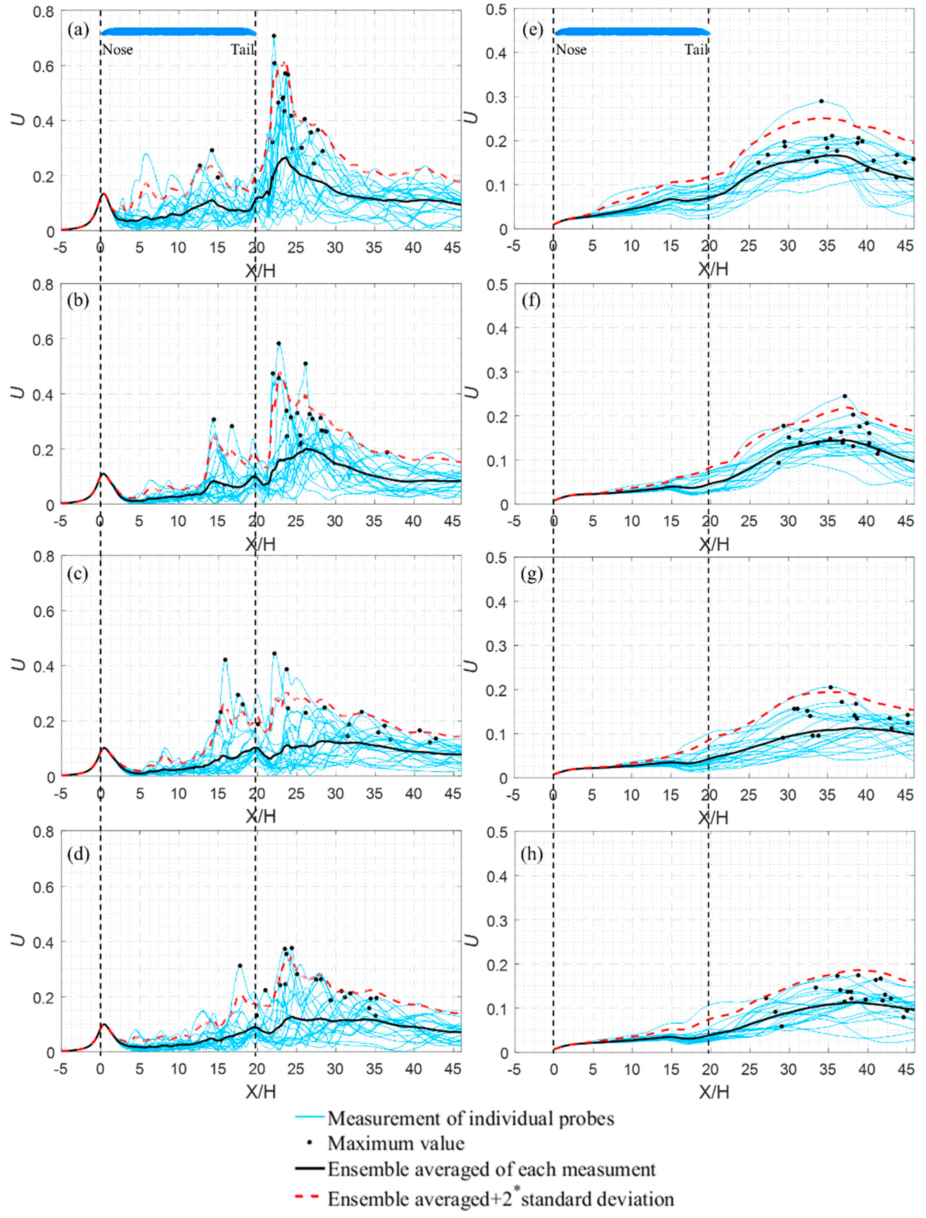
where represents the average maximum of the 1 s moving average (1s MA) of 20 individual runs, and σ represents the standard deviation of the 1s MA maximum. The characteristic velocity U2σ represents the maximum slipstream velocity that may occur at the measurement position within a 95% confidence interval. Generally, at least 20 individual runs are needed to calculate the characteristic velocity U2σ. To meet the requirements, 20 individual runs are selected as the measurement data in this study. The raw data and the 1s MA are shown as blue solid lines on the left- and right-hand sides of Figure 15, respectively. The ensemble average of the raw data and the ensemble average of the 1s MA are shown as the black solid lines on the left- and right-hand sides of Figure 15, respectively. The U2σ values of the raw data and of the 1s MA are shown by the red dashed line on the left- and right-hand sides of Figure 15, respectively. Table 3 shows the U2σ values without and with 1s MA, and the U2σ value of the 1s MA is the “TSI” value of the different nose lengths on the trackside position. Whether with or without the 1s MA, the value of U2σ decreases with increasing nose length. The nose length increases from 4 to 12 m, and the U2σ values without and with 1 s MA decrease by 46.5% and 28.1%, respectively. Among these, the nose length increases from 4 to 7 m and the average U2σ value of 1s MA decreases by 16%. This shows that the influence of slipstream velocity on the surrounding environment can be effectively reduced by properly increasing the nose length.

Figure 15.
Instantaneous horizontal velocity for 20 individual runs at trackside position. Blue solid line: ensemble average of individual probes. Black solid line: ensemble average. Red dashed line: ensemble average + 2* standard deviation. Black dashed line: nose and tail. (From top to bottom: 4, 7, 9, and 12 m. Left: without 1 s moving average (MA); right: with 1 s MA).

Table 3.
Peak values of gust measurement without and with 1 s MA.
4.4. Flow-Field Visualization
4.4.1. Slipstream and Pressure
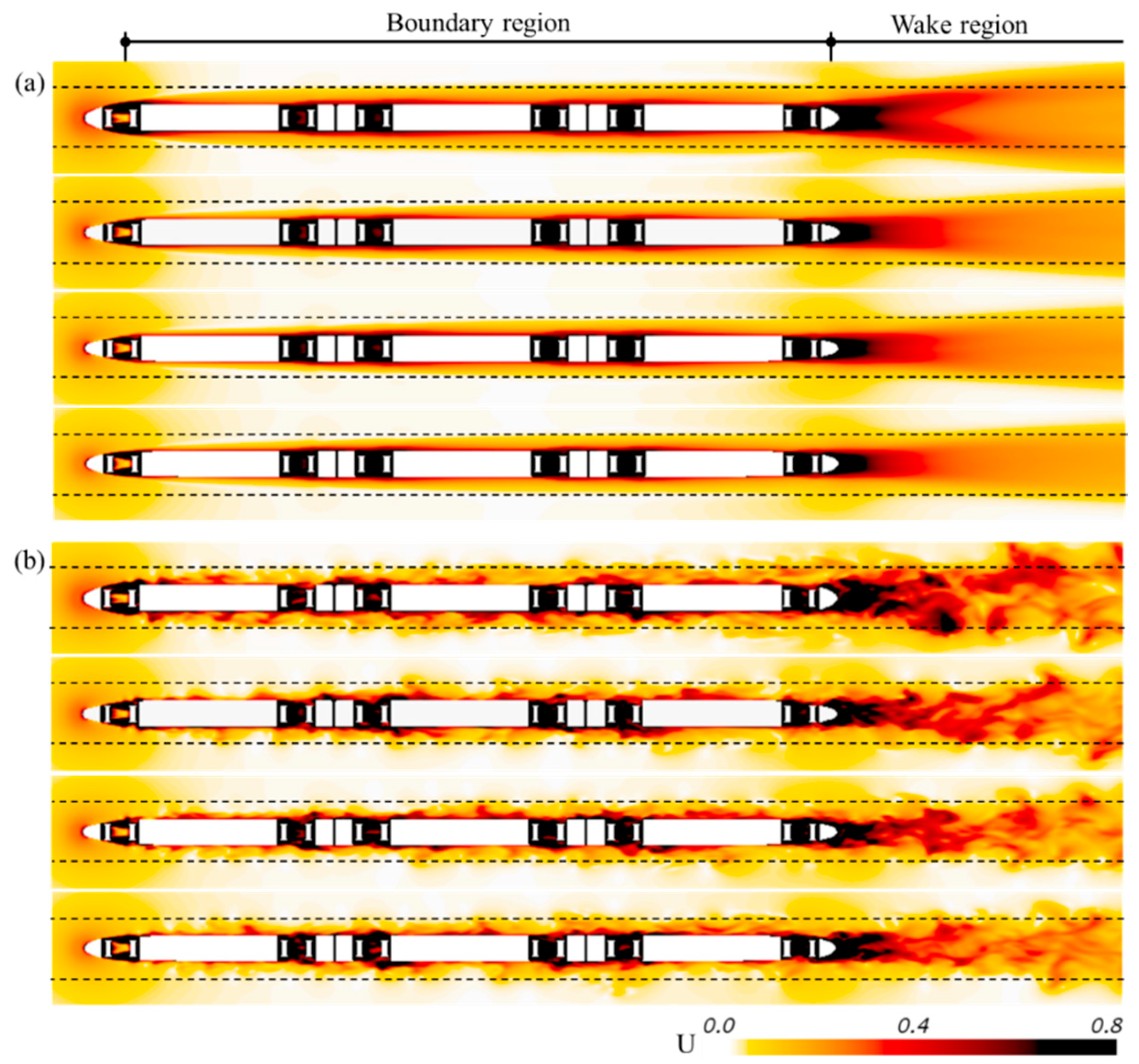
The slipstream velocities at 0.2 and 1.4 m from the TOR and different positions from the COT are quantitatively analyzed. Next, the contour plots of U at 0.2 m from the TOR will be studied. The time-averaged U and instantaneous U at a distance of 0.2 m from the TOR are shown in Figure 16. The flow field is divided into two regions: the boundary-layer region (covering the train) and the wake region. It can be seen from the Figure 16a that the time-averaged U and the instantaneous U near the nose of the tail car are relatively large. The nose length has a great influence on the development of the flow field along the train, especially on the wake-flow field. When the nose length is 4 m, the time-averaged U appears as a “bifurcation” in the wake region, but when the nose length is 7, 9, and 12 m the “bifurcation” is not obvious. This may be why the peak value of the time-averaged U for a nose length of 4 m is significantly larger than that of the other lengths in the wake region. Figure 16b shows an instantaneous U flow field. Similarly, in the wake region, a nose length of 4 m fluctuates more violently in the lateral direction, and the lateral pulsation decreases obviously with increasing nose length.
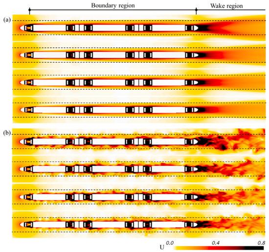
Figure 16.
Slipstream velocity at height of 0.2 m from TOR. (a) Time-averaged U, and (b) instantaneous U (from top to bottom: 4, 7, 9, and 12 m. Black dashed line is 3 m from COT.).
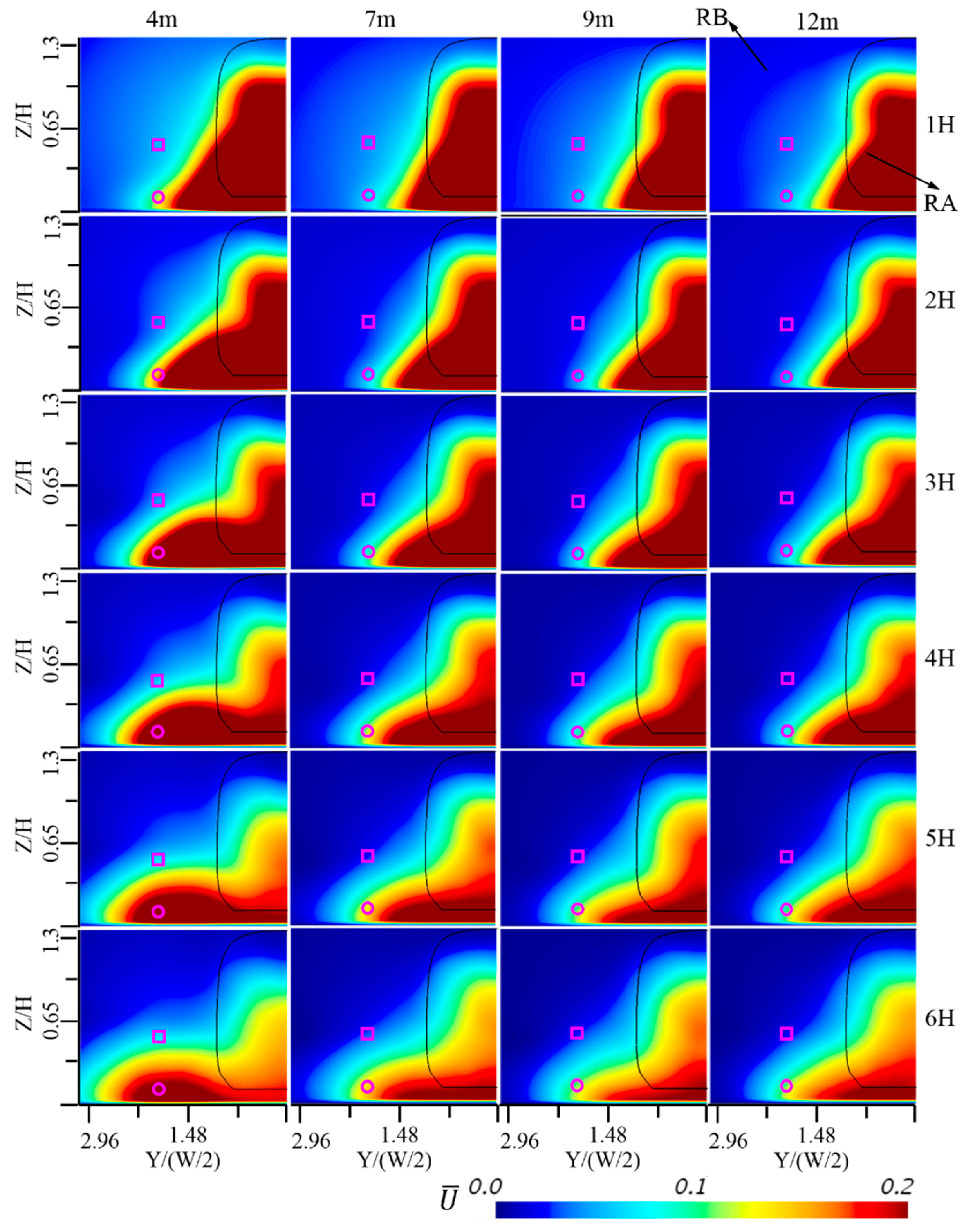
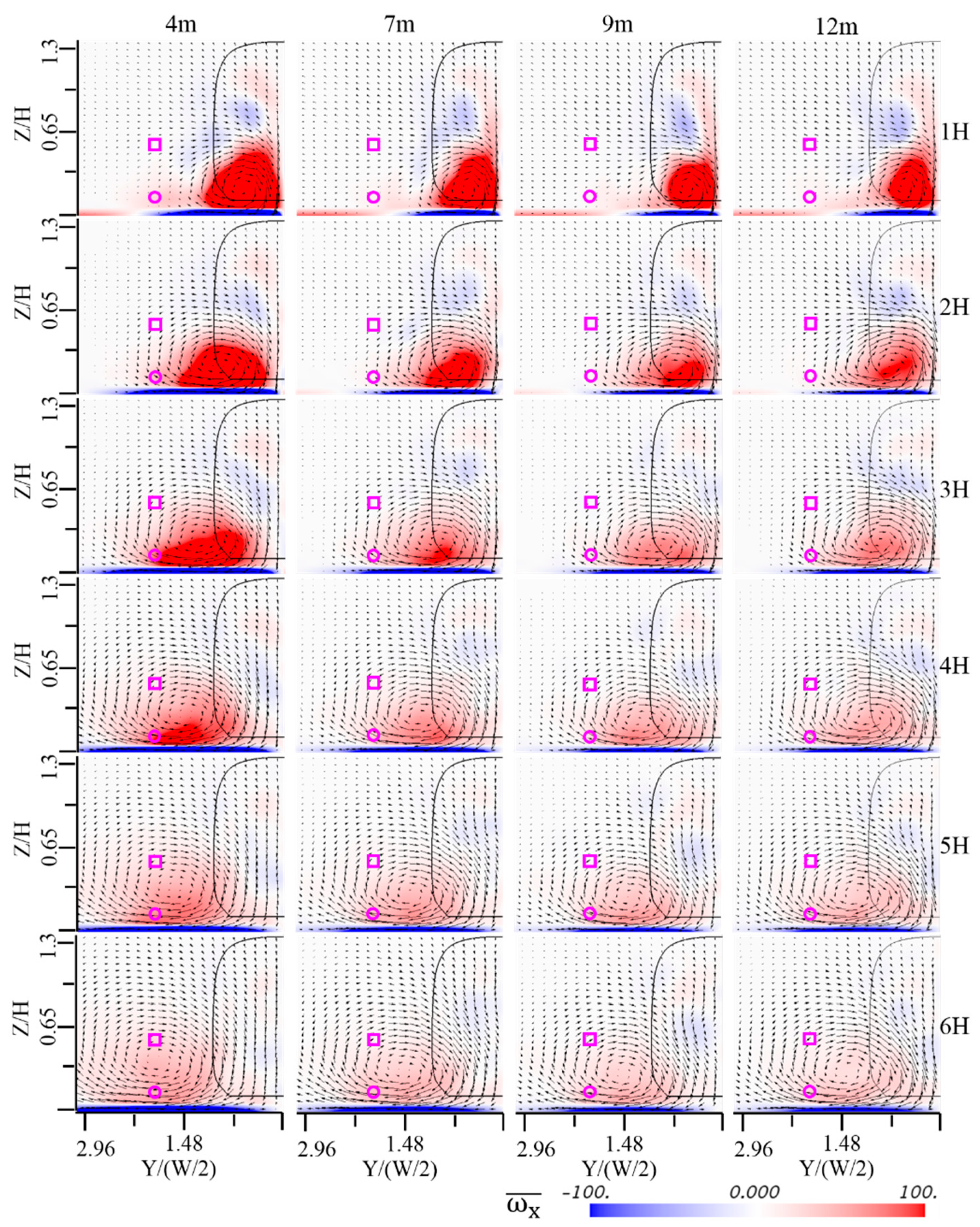
Figure 17 shows the time-averaged U of vertical planes 1 H, 2 H, 3 H, 4 H, 5 H, and 6 H from the tail of the train. Because the left- and right-hand sides are symmetrical, half of the plane is selected for the study. It can be seen from the figure that the time-averaged U in the vertical plane near the COT (RA) is larger than other regions (RB) with different nose lengths, and the RA shows the law of continuous downward and outward development, which is similar to the development of wake vortices [17]. At 1H, when the nose length is 4 m, the area of the RA is obviously larger than that of other nose lengths, so that the RA is closer to the trackside position and platform position, and causes the time-averaged U of the train with a nose length of 4 m to be greater than that of the other nose lengths. At 2 H, 3 H, 4 H, 5 H, and 6 H, there is a similar law. When the nose length of the train is 4 m, the RA already reaches the platform position, while the other nose length of the RA is only constantly approaching. This is also the reason for the law illustrated in Figure 10, in which the time-averaged U with a nose length of 4 m is significantly larger in the wake region.
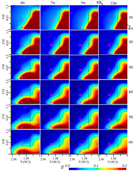
Figure 17.
Time-averaged U of vertical planes 1 H, 2 H, 3 H, 4 H, 5 H, and 6 H from tail of train (hollow pink square: platform position; hollow pink circle: trackside position.).
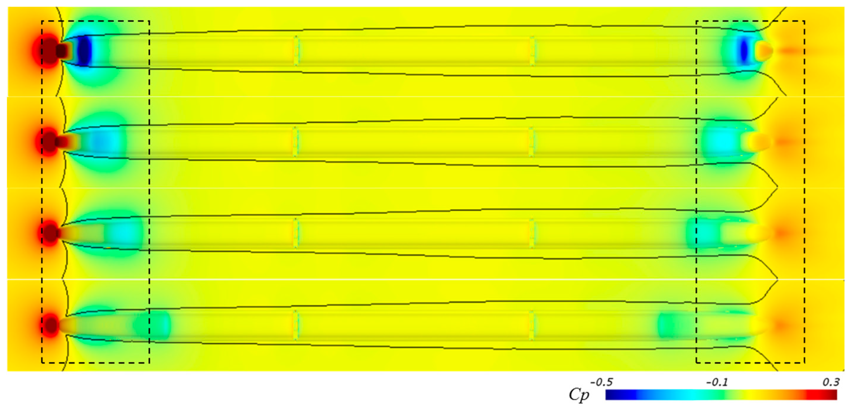
Figure 18 shows the contour plots of pressure on the surface of the train and plane at 1.6 m from the TOR. It can be seen from the figure that the streamlined length has a great influence on the distribution and amplitude of the surface pressure in the nose area of the train. With increasing nose length, the negative pressure concentration area at the junction of the streamlined and the non-streamlined nose of the head and tail cars moves backward. The amplitude of the negative pressure with a nose length of 4 m is still significantly larger, which is also consistent with the results plotted in Figure 14. Because of the difference of the nose length of the train, the distribution of the spatial pressure is also affected. Near the nose tip of the head car, the shorter the nose length, the larger the area of the pressure distribution area. Owing to the influence of the nose length, the pressure distribution on both sides of the streamlined head of the head and tail cars is also affected. It also has a great influence on the wake pressure distribution. The solid black line in the figure indicates the incoming flow velocity of 0.99 times, that is, 0.99 U∞, in which the surface layer of the train surface is δ0.99 near the train surface. Because the aerodynamic drag is composed of pressure drag and viscous drag, the thickness of the boundary layer has a greater impact on the viscous drag [30]. It can also be seen from the figure that a black solid line is formed in front of the head car, and the shape of the head car has a great influence on the formation of the black solid line. The formation of the black solid line with a nose length of 4 m is farther from the tip of the nose. The boundary-layer thickness of the train for all nose lengths increases gradually along the train. At the wake, the lateral width of the black solid line first increases and then decreases, and continues to develop backward. The shorter the nose length, the wider the lateral distance between the two lines.
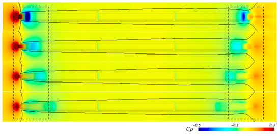
Figure 18.
Time-averaged pressure at a height of 1.6 m from TOR (from top to bottom: 4, 7, 9, and 12 m).
4.4.2. Wake Flows
Figure 19 shows time-averaged velocity vectors of vertical planes 1 H, 2 H, 3 H, 4 H, 5 H, and 6 H from the tail of the train. It can be seen from the figure that with increasing distance from the tail car the time-averaged velocity vectors of vertical planes with different nose lengths also show the law of continuous downward and outward development, and the radius of the vortex increases. However, the nose length has a great influence on the time-averaged velocity vector of the tail. At the same position from the tail car, when the nose length of the train is 4 m, the vortex radius is obviously larger than that of the other nose lengths, and the vortex center is higher from the ground and closer to the trackside position and the platform position. As a result, the time-averaged U with a nose length of 4 m is larger in the near-wake region. With increasing distance from the tail car, the time-averaged x-vorticity () decreases with increasing nose length. However, at the same location, for a nose length of 4 m is significantly larger than that of other nose lengths.

Figure 19.
Time-averaged velocity vectors of vertical planes 1 H, 2 H, 3 H, 4 H, 5 H, and 6 H from tail of train, colored by time-averaged x-vorticity (hollow pink square: platform position; hollow pink circle: trackside position).
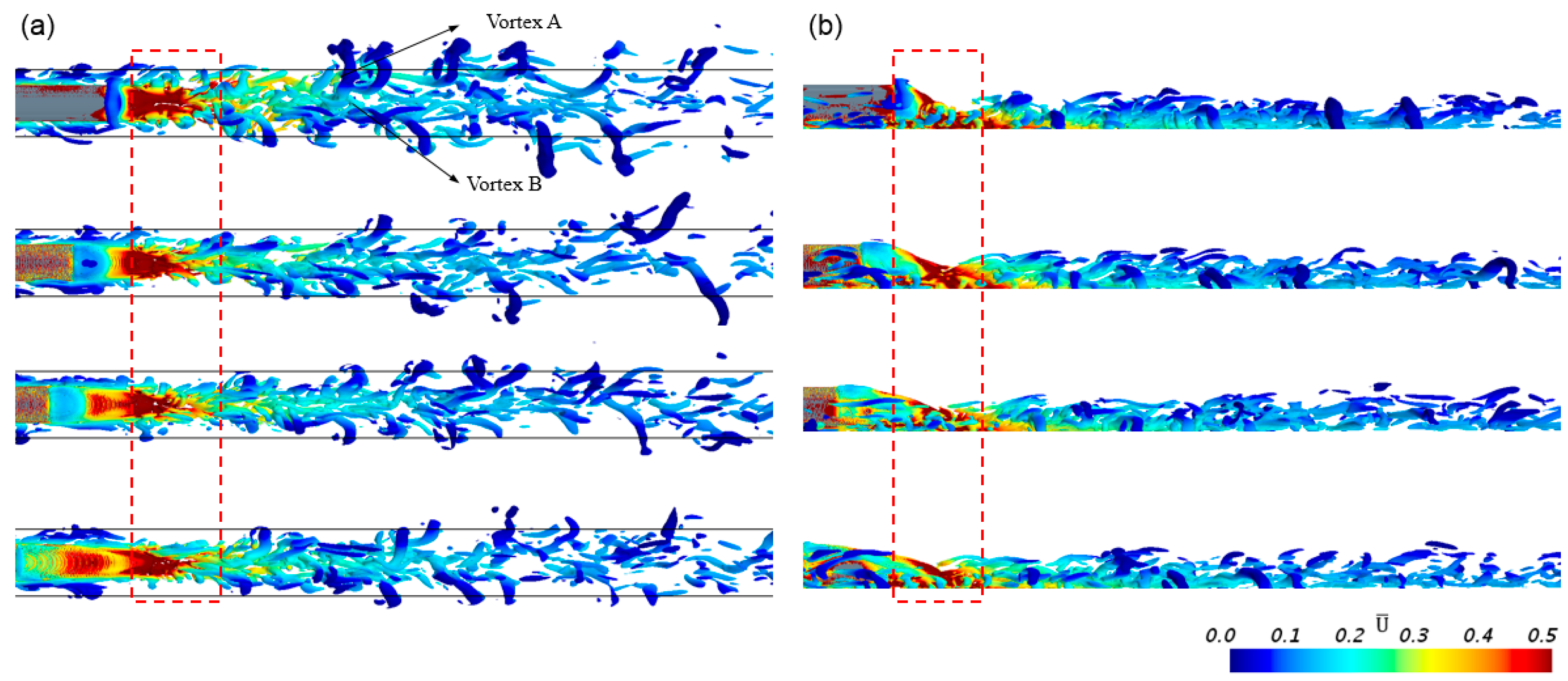
In the wake of the train, there are two vortices with opposite rotation direction that continue to develop downward and outward, and the appearance of the peak value of U is related to the two wake vortices [17]. At present, a large number of scholars use the Q criterion to study the development and separation of wake structures along HSTs [34,35,36,37]. The iso-surface of the second invariant of the velocity gradient tensor Q is defined as follows [36]:
where Ω is the rate-of-rotation tensor and S is the rate-of-strain tensor. Figure 20 shows a Q (Q = 5000) iso-surface with the time-averaged U colored according to the flow of different nose lengths at the wake. It can be seen from the figure that there are two vortices with opposite rotation direction in the wake of the four nose lengths, and the U value near the nose tip of the tail car is relatively large. The black line distance COT is 3 m. It can be seen from the figure that the nose length increases from 4 to 12 m, and the fluctuation of the wake vortex narrows in the lateral direction. In particular, when the nose length is 4 m it can be seen that the fluctuation of the vortex structure in the lateral direction is obviously wider and more intense. This may be the reason why the U value of a HST with a nose length of 4 m in the near-wake region is larger than that of other nose lengths. At the same time, in the longitudinal direction the nose length is longer and the wake vortex shedding distance is farther, and the wake vortex with nose lengths of 9 and 12 m is obviously longer than that with a nose length of 4 m. This may cause the U value of a nose length of 4 m to be smaller than those of nose lengths of 7, 9, and 12 m in the far-wake region, as can also be seen in Figure 9. In the vertical direction, with increasing nose length, the height of the vortex near the nose tip of the tail car is lower.
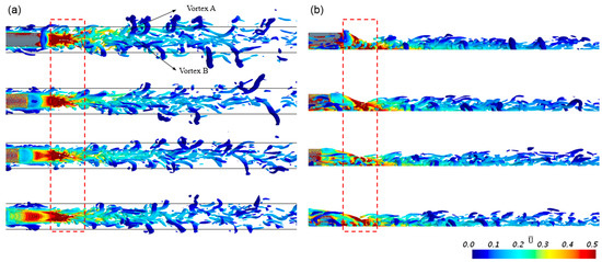
Figure 20.
Instantaneous iso-surface plot of Q criterion (Q = 5000) colored by time-averaged U: (a) top view and (b) side view (from top to bottom: 4, 7, 9, and 12 m. Black line is 3 m from COT).
5. Conclusions
In this study, the IDDES method is used to study the flow field around a HST with different nose lengths (4, 7, 9, and 12 m). The research includes time-averaged and instantaneous slipstream velocity, time-averaged pressure, wake flow, and aerodynamic force. From the results of the aforementioned factors, we can draw the following conclusions:
- (1)
- When the nose length increases from 4 to 7 m, the drag and lift force coefficients change obviously, in which the head car drag coefficient decreases by 17.6%, the tail car drag coefficient decreases by 29.3%, the head car lift force coefficient decreases by 15.8%, and the tail car lift force coefficient decreases by 75.7%. When the nose length increased from 7 to 12 m, the difference between drag and lift force coefficients was not obvious.
- (2)
- With increasing nose length, the peak value of time-averaged U in the same position decreases. When the nose length increases from 4 to 12 m, the peak value of time-averaged U in the trackside position decreases by 57%, and the peak value of time-averaged U in the platform position decreases by 19.5%. With increasing distance from the COT, the peak value of time-averaged U decreases. The maximum U value of the trackside position appears in the near wake, while the maximum U value of the platform position appears in the nose region. The slipstream is usually evaluated by characteristic velocity U2σ. In this study, the characteristic velocity U2σ of the trackside position is studied. It is found that the characteristic velocity U2σ decreases with increasing nose length. When the nose length increases from 4 to 12 m, the U2σ value decreases by 28.1%.
- (3)
- For the measuring points of trains with different nose lengths in different positions, the maximum value of ΔCP appears in the nose region. With increasing nose length, the ΔCP values of the measuring points at different positions decrease continuously. For ΔCP max, |ΔCP min|, and ΔCP at a height of 1.6 m from the TOR, the nose length increases from 4 to 12 m, which decreases by 26.5%, 58.5%, and 44.8%, respectively, with increasing nose length.
- (4)
- The nose length also has a great impact on the wake flow of the train. When the nose length is 4 m, the lateral fluctuation of instantaneous U and wake vortex is more intense, and the lateral fluctuation is also wider and more intense. When the nose length is longer, the shedding distance of the wake vortex is longer in the longitudinal direction.
Author Contributions
X.L. conceived, designed, collected and analyzed data, and wrote and revised the paper; G.C. provided guidance on numerical simulation software; D.Z. finalized the manuscript and provided the funding; Z.C. provided the train model.
Funding
This research was funded by the National Key R&D Program of China under grant numbers 2016YFB1200601-B14; and the Project of Innovation driven Plan in Central South University, grant number 1053320182352.
Acknowledgments
The authors acknowledge the computing resources provided by the High-Speed Train Research Centre of Central South University, China.
Conflicts of Interest
The authors declare no conflict of interest.
References
- Tian, H.Q. Train Aerodynamics, 1st ed.; China Railway Publishing House: Beijing, China, 2007; pp. 214–215. [Google Scholar]
- Zhang, J.; Wang, J.B.; Wang, Q.X.; Xiong, X.H.; Gao, G.J. A study of the influence of bogie cut outs’ angles on the aerodynamic performance of a high speed train. J. Wind Eng. Ind. Aerodyn. 2018, 175, 153–168. [Google Scholar] [CrossRef]
- Niu, J.Q.; Wang, Y.M.; Zhang, L.; Yuan, Y.P. Numerical analysis of aerodynamic characteristics of high-speed train with different train nose lengths. Int. J. Heat Mass. Trans. 2018, 127, 188–199. [Google Scholar] [CrossRef]
- Krajnović, S. Shape optimization of high-speed trains for improved aerodynamic performance. Proc. Inst. Mech. Eng. Part F J. Rail Rapid Transp. 2009, 223, 439–451. [Google Scholar] [CrossRef]
- Yao, S.B.; Guo, D.L.; Sun, Z.X.; Chen, D.W.; Yang, G.W. Parametric design and optimization of high speed train nose. Optim. Eng. 2016, 17, 605–630. [Google Scholar] [CrossRef]
- Vytla, V.V. Multidisciplinary Optimization Framework for High Speed Train using Robust Hybrid GA-PSO Algo. Ph.D. Thesis, Wright State University, Dayton, OH, USA, 2011. [Google Scholar]
- Howe, M.S. The genetically optimized tunnel entrance hood. J. Fluid Struct. 2007, 23, 1231–1250. [Google Scholar] [CrossRef]
- Muñoz-Paniagua, J.; García, J.; Crespo, A. Genetically aerodynamic optimization of the nose shape of a high-speed train entering a tunnel. J. Wind Eng. Ind. Aerodyn. 2014, 130, 48–61. [Google Scholar] [CrossRef]
- Jakubek, D.; Wagner, C. Shape optimization of train head cars using adjointbased computational fluid dynamics. In Proceedings of the First International Conference on Railway Technology: Research, Development and Maintenance, Las Palmas de Gran Canaria, Spain, 18–20 April 2012; Pombo, J., Ed.; Civil-Comp Press: Stirlingshire, UK, 2012. [Google Scholar]
- Munoz-Paniagua, J.; García, J.; Crespo, A.; Laspougeas, F. Aerodynamic Optimization of the Nose Shape of a Train Using the Adjoint Method. J. Appl. Fluid Mech. 2015, 8, 601–612. [Google Scholar] [CrossRef]
- Hemida, H.; Krajnović, S. LES study of the influence of the nose shape and yaw angles on flow structures around trains. J. Wind Eng. Ind. Aerodyn. 2010, 98, 34–46. [Google Scholar] [CrossRef]
- Chen, Z.W.; Liu, T.H.; Jiang, Z.H.; Guo, Z.J.; Zhang, J. Comparative analysis of the effect of different nose lengths on train aerodynamic performance under crosswind. J. Fluid Struct. 2018, 78, 69–85. [Google Scholar] [CrossRef]
- Xie, T.Z.; Liu, T.H.; Chen, Z.W.; Li, W.H.; Chen, X.D.; Zhou, X.S. Assessment and analysis on variation of trackside pressure induced by trains with different head shapes. J. Chin. Railw. Soc. 2019, 41, 41–49. (In Chinese) [Google Scholar]
- Cheli, F.; Ripamonti, F.; Rocchi, D.; Tomasini, G. Aerodynamic behaviour investigation of the new EMUV250 train to cross wind. J. Wind Eng. Ind. Aerodyn. 2010, 98, 189–201. [Google Scholar] [CrossRef]
- Bell, J.R.; Burton, D.; Thompson, M.C.; Herbst, A.H.; Sheridan, J. The effect of tail geometry on the slipstream and unsteady wake structure of high-speed trains. Exp. Therm. Fluid Sci. 2017, 83, 215–230. [Google Scholar] [CrossRef]
- Zhang, Z.Z.; Zhou, D. Wind tunnel experiment on aerodynamic characteristic of streamline head of high speed train with different head shapes. J. Cent. South Univ. 2013, 44, 2603–2608. [Google Scholar]
- Bell, J.R.; Burton, D.; Thompson, M.; Herbst, A.; Sheridan, J. Wind tunnel analysis of the slipstream and wake of a high-speed train. J. Wind Eng. Ind. Aerodyn. 2014, 134, 122–138. [Google Scholar] [CrossRef]
- Meng, S.; Zhou, D.; Wang, Z. Moving model analysis on the transient pressure and slipstream caused by a metro train passing through a tunnel. PLoS ONE 2019, 14, e0222151. [Google Scholar] [CrossRef]
- Flynn, D.; Hemida, H.; Baker, C.J. On the effect of crosswinds on the slipstream of a freight train and associated effects. J. Wind Eng. Ind. Aerodyn. 2016, 156, 14–28. [Google Scholar] [CrossRef]
- Rocchi, D.; Tomasini, G.; Schito, P.; Somaschini, C. Wind effects induced by high speed train pass-by in open air. J. Wind Eng. Ind. Aerodyn. 2018, 173, 279–288. [Google Scholar] [CrossRef]
- Wang, S.B.; Bell, J.R.; Burton, D.; Herbst, A.H.; Sheridan, J.; Thompson, M.C. The performance of different turbulence models (URANS, SAS and DES) for predicting high-speed train slipstream. J. Wind Eng. Ind. Aerodyn. 2017, 164, 46–57. [Google Scholar] [CrossRef]
- Wang, S.B.; Burton, D.; Herbst, A.H.; Sheridan, J.; Thompson, M.C. The effect of the ground condition on high-speed train slipstream. J. Wind Eng. Ind. Aerodyn. 2018, 172, 230–243. [Google Scholar] [CrossRef]
- Xia, C.; Wang, H.F.; Shan, X.H.; Yang, Z.G.; Li, Q.L. Effects of ground configurations on the slipstream and near wake of a high-speed train. J. Wind Eng. Ind. Aerodyn. 2017, 168, 177–189. [Google Scholar] [CrossRef]
- Shur, M.L.; Spalart, P.R.; Strelets, M.K.; Travin, A.K. A hybrid RANS-LES approach with delayed-DES and wall-modelled LES capabilities. Int. J. Heat Fluid Flow 2008, 29, 1638–1649. [Google Scholar] [CrossRef]
- Spalart, P.R.; Deck, S.; Shur, M.L.; Squires, K.D.; Strelets, M.K.; Travin, A.K. A new version of detached-eddy simulation, resistant to ambiguous grid densities. Theor. Comp. Fluid Dyn. 2006, 20, 181–195. [Google Scholar] [CrossRef]
- CEN European Standard. Part 6: Requirements and Test Procedures for Aerodynamics on Open Track. In Railway Applications-Aerodynamics; CEN EN 14067-6; BSI Standards Limited: London, UK, 2010. [Google Scholar]
- CEN European Standard. Part 4: Requirements and Test Procedures for Aerodynamics on Open Track. In Railway Applications-Aerodynamics; CEN EN 14067-4; BSI Standards Limited: London, UK, 2013; Available online: https://infostore.saiglobal.com/preview/is/en/2013/i.s.en14067-4-2013.pdf?sku=1694040 (accessed on 28 October 2019).
- Baker, C.J.; Jones, J.; Lopez-Calleja, F.; Munday, J. Measurements of the cross wind forces on trains. J. Wind Eng. Ind. Aerodyn. 2004, 92, 547–563. [Google Scholar] [CrossRef]
- Niu, J.Q.; Zhou, D.; Liu, T.H.; Liang, X.F. Numerical simulation of aerodynamic performance of a couple multiple units high-speed train. Veh. Syst. Dyn. 2017, 55, 681–703. [Google Scholar] [CrossRef]
- Niu, J.Q.; Zhou, D.; Liang, X.F. Numerical simulation of the effects of obstacle deflectors on the aerodynamic performance of stationary high-speed trains at two yaw angles. Proc. Inst. Mech. Eng. Part F J. Rail Rapid Transp. 2018, 232, 913–927. [Google Scholar] [CrossRef]
- Baker, C.J. The flow around high speed trains. J. Wind Eng. Ind. Aerodyn. 2010, 98, 277–298. [Google Scholar] [CrossRef]
- CEN European Standard. Part 4: Requirements and Test Procedures for Aerodynamics on Open Track. In Railway Applications-Aerodynamics; EN 14067-4:2005+A1; BSI Standards Limited: London, UK, 2009; Available online: https://www.google.com.hk/url?sa=t&rct=j&q=&esrc=s&source=web&cd=1&cad=rja&uact=8&ved=2ahUKEwi435acpb7lAhWDxIsBHSM4CKYQFjAAegQIBRAC&url=http%3A%2F%2Fgost-snip.su%2Fdownload%2Fbds_en_14067_4_2005_a1_2009_railway_applications_aerodynamic&usg=AOvVaw34ZkFIe61QJ8LqDEWd8fR- (accessed on 28 October 2019).
- European Union Agency for Railways. Commission Regulation (EU) No 1302/2014 concerning a technical specification for interoperability relating to the ‘rolling stock — locomotives and passenger rolling stock’ subsystem of the rail system. Off. J. Eur. Union 2014, 356, 288–290. [Google Scholar]
- Chen, G.; Li, X.B.; Liu, Z.; Zhou, D.; Wang, Z.; Liang, X.F.; Krajnovic, S. Dynamic analysis of the effect of nose length on train aerodynamic performance. J. Wind Eng. Ind. Aerodyn. 2018, 184, 198–208. [Google Scholar] [CrossRef]
- Zhang, J.; He, K.; Xiong, X.H.; Wang, J.B.; Gao, G.J. Numerical Simulation with a DES Approach for a HighSpeed Train Subjected to the Crosswind. J. Appl. Fluid Mech. 2017, 10, 1329–1342. [Google Scholar]
- Munoz-Paniagua, J.; García, J.; Lehugeur, B. Evaluation of RANS, SAS and IDDES models for the simulation of the flow around a high-speed train subjected to crosswind. J. Wind Eng. Ind. Aerodyn. 2017, 171, 50–66. [Google Scholar] [CrossRef]
- Yao, Y.F.; Sun, Z.X.; Yang, G.W.; Liu, W.; Prasert, P. Analysis of Aerodynamic Noise Characteristics of High-Speed Train Pantograph with Different Installation Bases. Appl. Sci. 2019, 9, 2332. [Google Scholar] [CrossRef]
© 2019 by the authors. Licensee MDPI, Basel, Switzerland. This article is an open access article distributed under the terms and conditions of the Creative Commons Attribution (CC BY) license (http://creativecommons.org/licenses/by/4.0/).


