Abstract
Gait analysis is recognized as a method used in quantifying gait disorders and in clinical evaluations of patients. However, the current guidelines for the evaluation of post anterior cruciate ligament reconstruction (ACLR) patient outcomes are primarily based on qualitative assessments. This study aims to apply gait analyses and mathematical, index-based health management, using the Mahalanobis Taguchi System (MTS) and the Kanri Distance Calculator (KDC) to diagnose the level of the gait abnormality and to identify its contributing factors following ACLR. It is hypothesized that (1) the method is able to discriminate the gait patterns between a healthy group (HG) and patients with ACLR (PG), and (2) several contributing factors may affect ACLR patients’ rehabilitation performance. This study compared the gait of 10 subjects in the PG group with 15 subjects in the HG. The analysis was based on 11 spatiotemporal parameters. Gait data of all subjects were collected in a motion analysis laboratory. The data were then analyzed using MTS and KDC. In this study, two significant groups were recognized: the HG, who achieved results which were within the Mahalanobis space (MS), and (ii) the PG who achieved results above the MS. The results may be seen as being on-target and off-target, respectively. Based on the analysis, three variables (i.e., step width, single support time, and double support time) affected patient performance and resulted in an average mark of above 1.5 Mahalanobis distance (MD). The results indicated that by focusing on the contributing factors that affect the rehabilitation performance of the patients, it is possible to provide individualized and need-based treatment.
1. Introduction
Gait analysis aims to determine the factors that influence a person to walk in the manner that he/she does. To accomplish this target, gait analysis involves the collection and investigation of qualitative data regarding the gait patterns of the individual. Gait analysis has been used in clinical settings for several disorders, including cerebral palsy, Parkinson’s disease, muscular dystrophy, osteoarthritis, rheumatoid arthritis, lower limb amputation, head injury, stroke, spinal cord injury, myelodysplasia, and multiple sclerosis.
This analytical method is widely used to organize surgery in the case of cerebral palsy and multiple joint disease, to produce unique insoles, to prescribe footwear, to schedule and monitor physiotherapy in various illnesses such as hemiplegia, to predict future issues such as foot ulceration in peripheral neuropathy, and to monitor the manufacturing and application of orthoses and prostheses.
For ACLR patients, the current guidelines for the evaluation of an ACLR patient’s results are primarily based on the clinician’s decisions and experience. These guidelines usually consist of a qualitative assessment of the early intervention plans that emphasizes the restoration of flexibility, muscular strength, and ligament stability by using closed kinetic chain exercises [1,2,3,4]. However, none of the post-ACLR rehabilitation guidelines included gait analysis as an examination or evaluation tool. It is unclear why this approach has been overlooked from the guidelines.
The Medical Outcomes Study 36-item Short Form (SF-36) is one of the most popular general health outcome measures used in the follow up of post-ACLR patients. The Knee Outcome Survey-Activities of Daily Living Scale (KOS-ADLS) can assess the functional limitations of the knee using a self-reporting mechanism. The Knee Injury and Osteoarthritis Outcome Score is the most effective for young and active individuals. The International Knee Documentation Committee 2000 Subjective Knee Evaluation Form can be used to assess patient improvement. Other commonly-used questionnaires included the Lysholm Knee Scale, the Cincinnati Knee Rating Scale, the Tegner Activity Level Scale, and the Marx Activity Level Scale [5,6].
These questionnaires and scores are based either entirely on the patient’s subjective opinions, on the clinician’s objective results using the test methods described earlier, or a mixture of both. However, subjective functionality and/or pain in certain operations do not indicate whether certain muscles are being used in certain operations. It is also not a good indicator to show if a person is at greater risk of developing osteoarthritis in the near future, even though he/she might be problem-free currently [7,8].
A major problem with this kind of subjective assessment is that the clinician’s capacity to provide safe and high-quality care relies on their ability to reason, think, and judge appropriately. These abilities and skills may be lacking among less experienced clinicians [9,10]. Furthermore, a number of exams need to be conducted to verify the medical diagnosis. The inclusion of a gait analysis may reduce the time required to achieve a diagnosis.
Recently, the use of medical apps in computerized intelligence systems is gaining importance. In addition, the implementation of computerized, health-related, decision support schemes represents a viable alternative to achieve a quick and precise medical diagnosis for patients. Therefore, medical information needs to integrate a classification approach with a mixed decision support scheme to facilitate digital access to health care information for healthcare professionals.
The Mahalanobis Taguchi System (MTS) is a new technique for diagnosing and predicting multivariate data [11,12,13,14,15,16]. MTS is a relatively new statistical method that incorporates several mathematical ideas. It is also used in the field of medical diagnoses and multidimensional system classifications [17,18,19,20]. For a relatively new technique, MTS is extremely effective, and it has been applied in a variety of fields [17,19,21]. For example, MTS has been incorporated in a variety of apps for healthcare diagnoses, fire detection, earthquake and weather forecasting, and loan rating prediction [11,13,22,23,24,25,26,27].
Furthermore, MTS is capable of eliminating any unnecessary items in the information system and providing useful data to assist healthcare professionals in decision making during diagnoses of diseases [28,29,30]. In addition, MTS is able to perform classification duties and recognize the significant multivariate system variables.
To significantly improve the process of discovering the most helpful parameters, the Kanri Distance Calculator (KDC) is incorporated into the MTS [31,32]. KDC-MTS is an extremely efficient approach to improve the accuracy of the predictive model. Both MTS and KDC are statistical methods that incorporate several mathematical ideas [6]. These techniques are used for diagnosing and predicting multivariate data [17,18,19,20]. Although many tools have been created to evaluate the patterns and dynamics of large data sets, only KDC allows users to understand exactly how far they are from the desired target state, and how each variable contributes to the entire distance from the target state. Apart from calculating connections among the factors within a general information set, KDC is also able to calculate the correlation between each of the factors mathematically [7]. With regard to MTS, this research implemented KDC to define the specific factors affecting the performance of post-ACLR patients.
Thus, data mining applications can be created by implementing a mathematical, index-based health management system to better recognize and monitor the states of gait abnormality among high-risk patients, to design suitable procedures, and to decrease the number of hospital admissions and claims.
For this study, ACLR patients from the Rehab and Physiotherapy Unit of Hospital Tuanku Fauziah at Kangar, Perlis were recruited. Ten patients, all male, with unilateral primary ACLR were chosen for the ACLR group (PG). All the patients underwent similar rehabilitation procedures, starting with passive and then active mobilization after surgery. Our goal is to apply gait analyses and mathematical, index-based health management (MTS and KDC) to diagnose the level of gait abnormality and to identify its contributing factors following ACLR.
2. Method
2.1. Mathematical, Index-Based Health Management System
A mathematical, index-based health management system describes the mathematical formulations of a health status index model. Health status index models have received a great deal of attention in recent years as a new quantitative approach for health planning and policy making. This study therefore proposes a new health management system (monitoring, diagnosis, and actions that should be taken based on findings). Equations are formulated to calculate ACLR health indexes and to determine the amount of health improvement produced by a health care program. This study aims to utilize mathematical formulations, including MTS as a diagnosis system and the Kanri Model as high impact prescription tool, to monitor, diagnose, and plan the actions to be taken based on the findings.
2.1.1. Mahalanobis–Taguchi System (MTS)
The Mahalanobis–Taguchi System (MTS), which was developed by Taguchi, is a diagnosis and forecasting technique for multivariate data [22,30]. MTS combines the Mahalanobis distance (MD) with Taguchi’s method (TM), and is used to optimize multidimensional systems [19].
Recent developments in the MTS have enhanced the diagnostic techniques with an assessment scale for data classification. In general, MD provides two categories, namely, ‘healthy’ or ‘normal’ and ‘abnormal’ groups of elements. MD is employed to distinguish the level of abnormality between the groups of elements. The abnormal group is different from the normal group in a few aspects. Elements that are in the normal or desirable form are considered to be normal data, whereas those that are undesirable are considered to be abnormal data. Depending on the acuteness levels of their abnormalities, abnormal elements may occasionally be categorized into groups [11]. The Signal to Noise (S/N) ratio is utilized to assess the efficiency of the system in the MTS, and OAs are employed to maximize the potential of the features that directly optimize the S/N ratio.
The Four Steps in MTS
The data are analyzed using the Mahalanobis–Taguchi System (MTS) [18], i.e., a combination of MD and Taguchi strategies. MD is a generalized distance that is useful to identify similarities between healthy and unhealthy sample sets. A scalar value is used to represent a multivariate system [33]. Taguchi strategies are statistical approaches used to enhance the engineered quality to make the system more powerful [28,34,35]. There are four steps in MTS [18]:
Step 0: Identification of assessment criteria and collection of patients’ spatiotemporal data
Step I: Mahalanobis space (MS) creation
Data from the healthy subjects are collected to create a standard data set. Their MDs constitute a reference space, called MS. Their MDs are approximately equal to one. In this study, a feature dataset consisting of spatiotemporal data from healthy subjects was used to create the MS. The healthy data set is denoted as H, is the observation on the feature, where and Then, and are the mean and standard deviations of the th feature respectively, where Each individual feature of each data vector () is normalized by the mean () and the standard deviation (). Hence, the normalized values are as follows:
where
The MDs of the healthy dataset are calculated with the following formula:
where is the transpose vector and is the inverse of the covariance coefficient matrix . We compute as:
Multicollinearity (strong correlations among features) is one issue that can be tackled with MD. Multicollinearities will have a problematic impact within a singular covariance coefficient matrix, resulting in an imprecise inverse of the covariance coefficient matrix, and subsequently producing an inaccurate MD [29]. MDA may be utilized to address this issue. MDA is MD corresponding to the adjoint matrix of the covariance coefficient matrix, as shown below:
where is the adjoint matrix of the covariance coefficient matrix . Since , the relationship between MD and MDA is given by:
Step II: Validation of MS
In this step, the trials of ACLR subjects are selected [13]. The abnormal data set is symbolized as P; is the observation of the feature, where and It is normalized by applying the mean and standard deviation of the healthy data set, while the MDs are estimated using the feature information and the coefficient matrix. MDs which correspond to the ACLR will be out of the MS if the MS is appropriately constructed. In other words, the MDs associated with abnormal conditions will have higher values [36,37].
Step III: Identification of useful features
The useful features are selected via the OAs and S/N ratios. In MTS, OAs are used to recognize the significant features by decreasing the number feature combinations which were initially established. The number of features determines the true number of columns in the OA. Two levels of factors are used: Level-1 indicates that the feature is included, while Level-2 means that it is not. To measure the accuracy of the MS predictions, S/N ratios are used. These are calculated using only the ACLR conditions. The equation for determining the S/N ratio () corresponding to the ith run of the OA is
where ith is the number of ACLR conditions and is the MD of the ACLR condition. By evaluating the gain in the S/N ratios, the useful features are identified. By using Equation (9), the gain of each feature is computed. Features with positive gains are considered useful.
Step IV: Future diagnosis
The MS is rebuilt using the attributes recorded in Step III, and the MDs of the monitored products are calculated. The subjects are healthy if the MDs are inside the MS. If the MDs are outside the MS, then the subjects reveal abnormal (ACLR) behavior. A greater MD indicates a greater deviation between healthy and ACLR patients [13].
2.1.2. Kanri Distance Calculator (KDCTM)
The proprietary combination of patented statistical and method techniques provided by the Kanri model offers an exceptionally strong capacity to assess big information sets with multiple variables [31,32,38,39]. While many instruments assess models and dynamics for big information sets, only KDCTM enables users to know where they are in relation to a required target state and the particular contribution of each variable to the general distance from the target state. The Kanri model is able to calculate the connection of the factors within the general information set. In addition, it can also determine mathematically the correlation between each of the factors [7].
The Kanri method aims to provide a multi-attribute (variables) management scheme to develop a multivariate measurement scale with which to measure the distances from a target or reference group that is described as effective. A root cause assessment (RCA) is conducted on an individual basis after the development, validation, and optimization of the measurement scale. For each attribute, we calculate contribution ratios (CRs) in the RCA so that we can concentrate on the characteristics with the highest impact.
Step V: Perform Root Cause Analysis (RCA)
RCA is performed to identify any abnormality in the influencing variables of a person [40]. The effect of the variables associated with the abnormality can be approximated by using the evaluation of variance [40,41]. The evaluation of variance assists us in discovering the efforts of factors for the general variant (abnormality) from the reference group or CG. In order to perform RCA, orthogonal arrays (OA) or any fractional factorial form design of the experimental matrix are utilized.
The purpose of using fractional factorial designs is to estimate the effects of several variables and the required interactions by reducing the number of trials. In RCA, the impact ratios (IR) of the variables are determined. In fractional factorial trials, a small percentage of the total number of trials is usually performed to decrease the price, time, and material. Primary results and chosen connections can end up being approximated with such fresh outcomes. The OA is an example of this [39,42,43].
Orthogonal Arrays (OAs)
OAs are extensively utilized in applications for robust engineering. In robust engineering, the principal purpose of OAs is to allow technical engineers to appraise a product design with regard to robustness against noise and cost. This is accomplished by altering the configurations of control factors. OA is normally an inspection tool to prevent a bad design from going ‘downstream’.
Arrays may have factors with many levels, although two- and three-level factors are commonly encountered. A Ls (2) array is shown in Table 1. This is normally a two-level array where the variables are different within the two levels. In this array, an optimum of eleven factors can be allocated. The twelve combinations with 2s and 1s correspond to the different variable combinations to be examined. 1s and 2s correspond to the presence (on) and absence (off) of the variable, respectively. As mentioned earlier, an analysis of the variance to calculate the impact proportions of the factors is performed in RCA. Since MD is usually a squared distance, and an analysis of variance cannot be performed on squared values, we need to make use of the square root of MD (WMD) for the evaluation, as shown in Table 1. WMD is denoted as D hereafter.

Table 1.
Physical layout of corresponding L12 (211) orthogonal array with 11 variables.
Impact Ratios (IRs)
Consider that an orthogonal array (or any fractional factorial experimental design) has r runs (variable combinations) and k + 1 columns. Let the k variables X1, X2, and Xk be allocated to the first k columns of this array, as shown in Table 2:
Table 2.
Fractional factorial design or orthogonal array with 12 runs and 11 columns.
The impact ratios are computed as follows:
where r = total number of runs
where
= sum of all Ds when X2 is ‘on’ in Table 2, = sum of all Ds when X2 is ‘off’ in Table 2, and r = total number of runs
In general,
where
= sum of all Ds when is ‘on’ in Table 2, = sum of all Ds when is ‘off’ in Table 2, and r = total number of runs
2.1.3. Integrated Approach
In this study, we proposed a combination MTS–KDC approach for health management. This approach included data collection on the gait of the individuals, and the health of each individual was determined by performing MD for each individual [19]. After that, the participants would be given a tailored prescription to improve their health, as demonstrated in Figure 1.
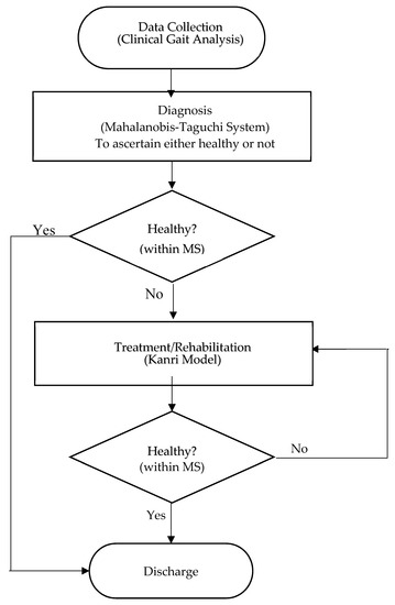
Figure 1.
Flow chart of integrated gait abnormality detection approach based on MTS and the Kanri model.
The data flow of the present study is shown in Figure 1. A patient is first examined using a gait analysis unit and/or procedure to obtain the values needed to derive certain scores, such as the Mahalanobis Distance (MD). The level of ACLR patient performance is then determined using the MD score. Patients with a MD value less than the Mahalanobis Space (MS) value would be considered as fully recovered, whereas patients with a MD value more than MS value would need to undergo further treatment. The useful features are then analyzed using the Taguchi Method. This method aims to reduce the number of required assessments by focusing only on essential factors. Finally, therapies are prescribed by using the Kanri Model.
2.2. Proposed Approach
We proposed an integrated approach using the MTS and Kanri Model to enhance the diagnosis and analysis of ACLR. This approach can be split into two phases: the first would use the MD to distinguish the routine ACLR, and would use OAs and the S/N ratios to select important features [13]; the second phase demonstrates how to use the model created in the initial phase and to identify contributing factors from the Kanri Model. A flow chart describing this strategy is shown in Figure 2. A broader description is given below.
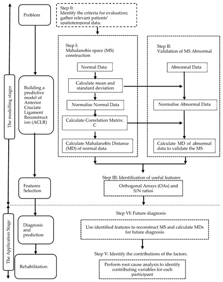
Figure 2.
Flow chart of the approach proposed in this study.
2.2.1. Modelling Stage
There are three steps in the model development; the first was to define the issue whereby the spatiotemporal gait parameters were identified. Next, we gathered the essential data to select a ‘normal’ or ‘healthy’ group to construct the MS. Following that, the information from the healthy group and the spatiotemporal gait parameters was used to get the Mahalanobis distance MS1, while data from the ACLR group and the chosen attributes were used to get the Mahalanobis distance MS2. Next, we identified an appropriate threshold to efficiently distinguish the healthy and ACLR groups. The final step involved the attribute selection, in which the vital features are chosen.
2.2.2. Application Stage
The developed model can be used to forecast the ACLR rehabilitation patterns by entering the ACLR data and the chosen features. In addition, at this stage, we can offer customized assessments and exercises based on the factors which affect the patients.
2.3. Case Study
Step 0: Identify the criteria for evaluation and gather patients’ relevant spatiotemporal data.
2.3.1. Participants
To assess the efficiency of the method in this study, ACLR patients from the Rehab and Physiotherapy Unit of Hospital Tuanku Fauziah at Kangar, Perlis were recruited for this study. Ten patients, all males, with unilateral primary ACLR were chosen for the ACLR group (PG). All patients underwent similar rehabilitation procedures, starting with passive and then active mobilization after surgery. Meanwhile, 15 healthy subjects were selected for the healthy group (HG) with the condition that they had no previous history of lower extremity injuries, surgery, or neuropathy. The HG consisted of 15 males. The height, age, and weight distribution of the two groups were not significantly different (p > 0.05) (Table 3). Ethical approval was granted by the University of Malaysia Perlis, and the participants provided written informed consent.
Table 3.
Anthropometric data of the subjects and p-value of relationship between the healthy group (HG) and ACLR group (PG). Values stated as mean ± standard deviation.
2.3.2. Procedures
Subjects were instructed to walk seven times on an 8m walkway. The first two laps were not measured to allow for familiarization with the task and instrumentation. The last five laps were assessed to capture the gait cycles, employing the dominant limb from the HG and the injured limb from the PG.
The trial was conducted in the Motion Lab at the University of Malaysia, Perlis. Motion data were collected using a motion capture system comprising five Oqus cameras (Oqus, Qualisys AB, Gothenburg, Sweden). A total of 36 reflective markers were placed on the joint landmarks and segments of the lower limb. Two force plates were reset for the next trial. The vertical ground reaction force was detected by two force plates with dimensions of 400 × 600 mm (Bertec, Worthington, Ohio, OH, USA) while the subject performed several walks at his own pace. At least five successful trials were collected and interpreted using the Qualisys Track Manager. The 11 spatiotemporal parameters (Table 4) of the trial were generated in Visual 3D Pro v6. This includes variations in the step width, stride speed, swing time, stance time, stride time, step time, step width, stride length, and step length.
Table 4.
Operational definitions of gait parameters and variables.
3. Results
3.1. Step I: Construction of MS
After collecting the necessary information (Table 5), we calculated the MD using the formulas in Section 2.2.1. To compute MD1, we utilized the HG data and the 11 selection features. The 15 healthy subjects were used as the benchmark (healthy) group. The average and standard deviation of every characteristic from the HG were computed, and the information from Table 5 was normalized using Equation (1). This normalized information was used to build the correlation matrix and its inverse. Next, the MDs were computed using Equation (4) as presented in Table 6. Likewise, using the inverse correlation matrix generated from the HG data, the MDs were computed for the 10 sets of PG data. The MDs of the HG were almost equal to one, as shown in Table 6.
Table 5.
Mean and standard deviation (SD) of healthy group (HG) and ACLR group (PG) for all variables.
Table 6.
MD of the healthy group (HG) data sets.
3.2. Step II: Validation of MS
In Step II of the MTS, the ACLR data were utilized to confirm the MS dimension scale. Using the average and standard deviation of the HG data, the PG data were normalized. The MDs of the ACLR group were computed using the covariance coefficient matrix of the HG data. From this study, the MDs were clearly out of the range of this MS, as shown in Figure 3. Therefore, the MS was valid. The 10 ACLR spatiotemporal data, along with the calculated MDs, are displayed in Table 7.
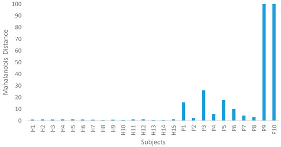
Figure 3.
Mahalanobis distance (MD) for the healthy group (HG) and ACLR group (PG).
Table 7.
MD for ACLR group (PG) data.
3.3. Step III: Identification of Useful Features
In Step III of the MTS, OAs and S/N ratios were used to examine the effects of every feature. Since 11 attributes were assembled, an L12 (211) OA was used. As revealed in Table 8 and Table 9, X1, X2, and X8 did not have a significant effect on the MD. Hence, the number of attributes was reduced from 11 to 8. The PG could be clearly distinguished from the HG group, as their MDs deviated significantly in the MS (PG: 2.308–1509.811, HG: 0.560–1.190).
Table 8.
L12 (211) OA for the ACLR conditions.
Table 9.
Average S/N ratios and gain for each feature.
3.4. Step IV: Future Diagnosis
The MS was reconstructed, and the MDs of monitored products were calculated using the useful features identified in Step III. If the MDs were within the MS, the monitored products were considered to be normal. If MDs were out of the MS, the monitored products exhibited abnormal behavior. The higher the MDs, the more deviation there was between the monitored product and the normal product.
The important set of variables can be identified at this stage using the OAs and S/N ratios. For the target groups, it is preferable to use a larger S/N ratio to generate MDs which are as large as possible. A L12 (211) OA was used, since 11 characteristics were built. There was no significant effect of X1, X2, and X8 on MD, as shown in Table 5. Therefore, the number of features decreased from 11 to 8. The threshold for MDs and MS was recalculated, incorporating only the useful features that were identified. Table 10 shows the updated MDs for both HG and PG.
Table 10.
MDs Value after recalculation using only the useful features.
3.5. Step V: Perform RCA
3.5.1. Orthogonal Arrays (OAs)
Orthogonal array (OA) was introduced as an approach utilized for the feature selection mechanism. OA incorporates the use of “1” and “2” for two-level factors, as shown in Table 11 and Table 12. This is normally a two-level array where the variables are different within two levels. In this array, an optimum of eleven factors can be allocated. The twelve combinations with 2s and 1s correspond to the different variable combinations to be examined. 1s and 2s correspond to the presence (on) and absence (off) of the variable, respectively.
Table 11.
L12 (28) OA of ACLR conditions.
Table 12.
Physical layout of corresponding to L12 (28) orthogonal array with 11 variables.
In this study, eleven variables were allocated to the first 11 columns of the orthogonal array. The last column was reserved for the responses of the combinations of the five variables. In the root cause analysis (RCA), the response was the MD corresponding to the variables in the respective combination (Table 11). The MDs in terms of the physical layout are listed in Table 11. For RCA, two-level arrays are preferred to ascertain the importance of the variables when the system is “on” and “off”; see Table 12. For the first combination, all variables were included, and MD was computed for a given participant. In the second combination, variables X3, X4, X5, X6, and X7 were used, and MD was computed with these five variables for the same participant. MDs for all other combinations were computed in a similar manner.
3.5.2. Impact Ratios (IRs)
Equations (10)–(16) were calculated for all participants, and IRs of all the variables for all the participants were obtained. Based on the example above, IRs were calculated for the 11 variables of all 10 participants. The results are shown in Table 13.
Table 13.
Analysis of the root cause by contribution ratios (percentages).
4. Discussion
A procedure for the health management of individuals comprises the following: (1) gather data about the health attributes of the individual, (2) calculate the gait abnormality value for the individual by determining the MD, and (3) offer the individual a high-effect prescription based on the health attributes to improve his/her health status [13,14,16,30,31,32,44].
In order to construct a measurement scale, it is necessary for a homogeneous data set from normal observations to be collected. This leads to the creation of a reference group called the normal group. In the scale, this group is used as a reference point. The collected normal datasets need to be standardized in order to obtain a dimensionless unit vector, followed by the MD computation. Practically, the MD for unknown data is interpreted as the closeness to the mean of the normal group. As a countercheck, it is necessary for the average value of the MDs for the normal group to be constantly close to unity. Therefore, they are called the normal space or Mahalanobis Space (MS) [18,27,30].
In order evaluate the measurement scale, observations made outside the MS or abnormal datasets are used.
The same mathematical calculation is repeated for the calculation of the same goal (MD value) using the abnormal sample data. However, the mean, standard deviation, and correlation matrix of the normal group determine the way the abnormal data is normalized. The normal MDs and abnormal MDs are then compared. An acceptable measurement scale should demonstrate significant differentiation between normal and abnormal MD values [18,27,30].
Different values of MD enable the group of HG and PG to be distinguished. The lower the value of the MD, the healthier the patient, as shown in Figure 3. This method also allows for a more objective assessment to be made of the patient’s state of health [30,31,32,38,44].
4.1. Diagnosis
In this approach, the level of abnormality is normally structured on a measure known as MD [12,13,14,16]. We needed to define the target group first. On a measurement scale in MS [5], the target group was used as a reference point. The target group in MS in this study was 15 healthy male subjects. Following the collection of the target group information, we calculated the MD using Equations (1)–(4).
The MD value was very small in the normal (healthy) dataset, and the average MD was near to 1. The abnormal (ACLR) MD values were greater than normal, illustrating the capacity of MD to classify the normal and abnormal values. Table 6 and Table 7 represent the MDs of normal and abnormal data, respectively.
Furthermore, this method was able to provide specific recommendations for therapy following knee operations. The MDs can be utilized to determine the best time for patients to return fully to sports activities.
It should be observed that the average value of the MD for ACLR individuals in Table 10 (typical MD = 130.429) was higher than that of the healthy individuals in Table 10 (average MD = 0.933). The patients could be rated in an ascending sequence based on the MD values. The results showed that for lower MD values, the deviation from healthy participants was likely lower, and thus, the patients would have an excellent likelihood of returning to work (RTW) [45]. From the results, subjects 2, 7, and 8 recorded MD values which were close to those of the healthy participants. For individuals with higher MD values, constant rehabilitation should be continued until reaching the ideal MD value [46].
4.2. Contributions of Variables
KDCTM is required to evaluate the effect of each parameter on the patient’s results. This can be done by using RCA to comprehend individual needs. The impact ratios (IRs) of the features were determined for all patients in this study using RCA [31,32,39,47]. In this way, we were able to define the contribution of the factors for each patient. Each candidate had a distinct distance variable effect. Table 13 outlines the contributing factors for the distances of the 10 patients being studied.
In Table 13, the RCA output shows the contributions of all the candidate distance variables. The output was structured to prioritize the greater distances in descending order. It enabled us to determine the contributing factors individually. Traditional analytics will emphasize this, and drive the conduct of the population. KDCTM offers a personalized driver perspective with each patient’s effects.
If viewed individually, P9 was heavily influenced by X4 and X9, which were the Stance Time and Double Support Time, respectively. As for P10, X6 and X9 affected the element in an abnormal way. This proved the importance of patient care tailored to each patient’s needs. The relationships established in this study can serve as a prescription for patients to consider corrective activities to decrease the influence of these factors on their general health. These essential features will be discussed in detail.
In terms of the parameters, X3 (step width) was the most important feature, followed by X6 (single support) and X9 (double support). X3 had the highest IR for P6 (69%), P3 (66%), P1 (62%), P4 (53%), and P5 (36%). The step width refers to the distance between the rear end of the right and left heel center lines along the mediolateral axis. A base of support domain was characterized by the step width and step width variability [48,49,50,51]. An increased step width indicates a loss of automaticity in walking that would render an individual more vulnerable to falling. Therefore, the step width is used as a parameter to evaluate the risk of falling and dementia. Under dual-task conditions, the step width can be also used to test the executive function in ACLR patients.
X3 variability reflected that step width had the highest IR for P1, P5, P3, P4, P6, P2, and P8. It can also be used to identify peripheral sensory impairments that lead to walking malfunction [52]. Other studies characterized increased step as a feature of ACLR patients who are fearful of falling, but also noted that the measure width itself is not a predictor of falling [53,54]. In comparison, decreased and increased step width variability were both linked to a history of falls. While the correlation between the step width variability of an ACLR knee and the drop risk is not clear, the results of this study revealed that the analysis of a base-of-support variable is justified [55,56].
The ACLR knees demonstrated reduced single support (X6) phases in comparison to healthy knees. This reflects the prolonged time in which the ACLR knees remain in flexion prior to maximum extension to prevent a sudden weight change. This adaptation mechanism has been also shown by an electromyography experiment, in which ACLR patients were shown to have prolonged firing of biceps, femoris, and vastus medialis during the stance phase in comparison to the HG [57].
X9 reflected Double Support, and had the highest IR for P10, P9, P4, and P2. The stance phase can be divided into sub phases, namely, first double support (both feet in contact with the floor), single support (one foot in contact with the floor), and second double support [58]. Compared with an uninjured leg, individuals with ACLR spent less time in double-limb support during late adaptation. However, the ACLR group was capable of adjusting this parameter in such a way that the PG leg spent an increased amount of time in double support during the de-adaptation period [59,60,61,62].
The differences in the double-support time are possibly related to the sensory alterations which emerge from a reconstructed knee. The problem was not corrected by medical procedures or therapy, and eventually, slow-adapting responses were formed as a response to repeated perturbations. An ACLR individual would attempt to reestablish the mechanical balance of the leg through therapy; thus, the common objective of therapy is to restore gross motion patterns. Comprehensive recovery of the physical functions of the reconstructed ACL requires reinnervation of free-of-charge nerve endings and mechanoreceptors, and the reestablishment of the ACLR reflex (hamstring activation after tibial translation) [59,63].
4.3. Customized Rehab Program
In identifying the contributing factors, it is crucial to have a tailored rehabilitation program for each patient. This ensures that individual issues of each patient can be addressed more specifically, and steps can be taken in a quicker manner to reduce the impact of the contributing factors. It was obvious from Table 13 that different patients had different numbers of impact factors.
For instance, X3 was a parameter that evaluated the risk of falling and of dementia. An increased step width indicated a loss of automaticity in walking which would make individuals more vulnerable to falls. Therefore, proprioceptive and balance training would be most relevant to such patients. By stimulating the proprioceptive and balance system through specific exercises, other mechanoreceptors of the knee joint would be stimulated to produce compensatory muscle activation patterns in the neuromuscular system, which may eventually improve joint stability [64,65,66].
As for X6 and X9, differences in the single/double-support time were related to the sensory alterations that emerged from reconstructed knees which led to slow-adapting responses as a result of repeated perturbations. In this case, muscular strength and endurance training might be most relevant for such patients. Specific muscle strength deficits depend on the graft type employed for ACLR (patellar tendon vs. semitendinosus/gracilis). Strengthening exercises, such as speed and specific muscular contractions, should be performed to overcome these deficits [67,68].
For patients with slower stride speeds (X11), the range of motion and flexibility training is more relevant. The slower stride speed of the ACLR was a result of the leg not being completely extended during the stance phase and at the end of the swing stage. Thus, it is vital to reestablish and maintain a full range of motion (ROM) of the knee. Quadriceps retraining was proven to increase ROM during the first phases. Achieving complete knee extension as soon as possible post-ACLR is not harmful to the graft or joint equilibrium; on the contrary, it might prevent patellofemoral pain and compensatory gait pathologies. It is strongly encouraged to incorporate a stretching program to maintain lower extremity flexibility [69].
To date, there is no curative treatment for ACLR. The rehabilitative process has been shown to be beneficial in regaining full knee extension, decreasing edema, and developing quadricep strength. However, extensive disabilities such as a decline in mobility may also occur during rehabilitation. Therefore, rehabilitation post-ACLR should shift from a protocol-based paradigm to an individual-tailored program. Many of the current studies do not evaluate the effectiveness of the aforementioned training in reducing the contributing factors of gait problems. Thus, future research is necessary to determine whether specific interventions targeting the contributing factors may improve gait biomechanics, and subsequently, reduce the gait abnormality following ACLR.
4.4. Limitations of the Study
Our study was limited to the effects of spatiotemporal parameters on gait performance. Although spatiotemporal facets are sufficient parameters to differentiate knee gait biomechanics between the ACLR and control groups, additional research is needed to evaluate kinetics, kinematics, and EMG parameters.
We only determined the contributions of variables for each patient. Additional research is needed to evaluate whether proposed exercise (proprioceptive and balance training, muscular strength and endurance training, range of motion and flexibility training) will provide more improvements.
The population being analyzed was relatively young, with an average age of 26 years and a low standard deviation. Conclusions from this study should be applied only to similar age groups, and future research on other age groups, especially older people, is required.
5. Conclusions
The present study provides a health management system for ACLR subjects. The system proposed by this study is useful in advancing rehabilitation performance. For example, the system can be incorporated as part of an integrated infrastructure built around a data capturing system. The system then allows for the automatic application of multivariate data and multidimensional mathematics to the data repository to perform specific commands or tasks, including the diagnosis of gait disorders. The development of such a rehabilitation monitoring system for doctors/physiotherapists has significant implications, as it allows healthcare professionals to make rapid decisions which are otherwise problematic when conventional rehabilitation diagnosis mechanisms are relied upon.
Author Contributions
All authors discussed and agreed upon the idea and made scientific contributions. H.S., N.A.A.O. and W.Z.A.W.M. designed the experiments and wrote the paper. H.S., M.S.A.M., M.H.F.R. and W.A.M. performed the experiments and analysed the data.
Funding
The study received financial support from Malaysia Ministry of Education through SLAI scholarship programme and from Platfom HIP-2 grant no.: AIM/PlaTCOM/HIP2/CCGF/2017/168.
Acknowledgments
The authors would like to express sincere gratitude to I.I.b.I. and A.b.A., supporting staff at Biomechanics Laboratory, Universiti Malaysia Perlis for their support. Special thanks to the Physioteraphy Unit of Hospital Tuanku Fauziah for providing physical therapy treatments for the subjects.
Conflicts of Interest
The authors declare no conflicts of interest.
References
- Konrath, J.M.; Saxby, D.J.; Killen, B.A.; Pizzolato, C.; Vertullo, C.J.; Barrett, R.S.; Lloyd, D.G. Muscle contributions to medial tibiofemoral compartment contact loading following ACL reconstruction using semitendinosus and gracilis tendon grafts. PLoS ONE 2017, 12, e0176016. [Google Scholar] [CrossRef] [PubMed]
- Drechsler, W.I.; Cramp, M.C.; Scott, O.M. Changes in muscle strength and EMG median frequency after anterior cruciate ligament reconstruction. Eur. J. Appl. Physiol. 2006, 98, 613–623. [Google Scholar] [CrossRef] [PubMed]
- Jenkins, P.J.; Clifton, R.; Gillespie, G.N.; Will, E.M.; Keating, J.F. Strength and function recovery after multiple-ligament reconstruction of the knee. Injury 2011, 42, 1426–1429. [Google Scholar] [CrossRef] [PubMed]
- Gokeler, A.; Benjaminse, A.; van Eck, C.F.; Webster, K.E.; Schot, L.; Otten, E. Return of normal gait as an outcome measurement in acl reconstructed patients. A systematic review. Int. J. Sports Phys. Ther. 2013, 8, 441–451. [Google Scholar]
- Kim, S.-J.; Yoon, J.-Y.; Kim, S.-M.; Ha, S.; Kim, S.-H.; Cho, I. A Comparative Study on the Postoperative Outcomes of Anterior Cruciate Ligament Reconstruction Using Patellar Bone–Tendon Autografts and Bone–Patellar Tendon–Bone Autografts. Arthrosc. J. Arthrosc. Relat. Surg. 2016, 32, 1072–1079. [Google Scholar] [CrossRef]
- Frank, R.M.; Mascarenhas, R.; Haro, M.; Verma, N.N.; Cole, B.J.; Bush-Joseph, C.A.; Bach, B.R. Closure of patellar tendon defect in anterior cruciate ligament reconstruction with bonee-patellar tendone-bone autograft: Systematic review of randomized controlled trials. Arthrosc. - J. Arthrosc. Relat. Surg. 2015, 31, 329–338. [Google Scholar] [CrossRef]
- Yu, P.V.; Wun, Y.; Yung, S.P. Role of Physiotherapy in Preventing Failure of Primary Anterior Cruciate Ligament Reconstruction. J. Orthop. Trauma Rehabil. 2017, 22, 6–12. [Google Scholar] [CrossRef]
- Winiarski, S.; Czamara, A. Evaluation of gait kinematics and symmetry during the first two stages of physiotherapy after anterior cruciate ligament reconstruction. Acta Bioeng. Biomech. 2012, 14. [Google Scholar]
- Lee, Y.C.; Teng, H.L. Predicting the financial crisis by Mahalanobis-Taguchi system - Examples of Taiwan’s electronic sector. Expert Syst. Appl. 2009, 36, 7469–7478. [Google Scholar] [CrossRef]
- Pal, A.; Maiti, J. Development of a hybrid methodology for dimensionality reduction in Mahalanobis–Taguchi system using Mahalanobis distance and binary particle swarm optimization. Expert Syst. Appl. 2010, 37, 1286–1293. [Google Scholar] [CrossRef]
- Wang, P.C.; Su, C.T.; Chen, K.H.; Chen, N.H. The application of rough set and Mahalanobis distance to enhance the quality of OSA diagnosis. Expert Syst. Appl. 2011, 38, 7828–7836. [Google Scholar] [CrossRef]
- Jin, X.; Chow, T.W.S. Anomaly detection of cooling fan and fault classification of induction motor using Mahalanobis–Taguchi system. Expert Syst. Appl. 2013, 40, 5787–5795. [Google Scholar] [CrossRef]
- Reséndiz, E.; Rull-Flores, C.A. Mahalanobis-Taguchi system applied to variable selection in automotive pedals components using Gompertz binary particle swarm optimization. Expert Syst. Appl. 2013, 40, 2361–2365. [Google Scholar] [CrossRef]
- Iquebal, A.S.; Pal, A.; Ceglarek, D.; Tiwari, M.K. Enhancement of Mahalanobis-Taguchi System via Rough Sets based Feature Selection. Expert Syst. Appl. 2014, 41, 8003–8015. [Google Scholar] [CrossRef]
- Muhamad, W.Z.A.W.; Ramlie, F.; Jamaludin, K.R. Mahalanobis-Taguchi system for pattern recognition: A brief review. Far East J. Math. Sci. 2017, 102, 3021–3052. [Google Scholar] [CrossRef]
- Taguchi, G.; Jugulum, R. The Mahalanobis–Taguchi Strategy; John Wiley & Sons: Hoboken, NJ, USA, 2002. [Google Scholar]
- Taguchi, G.; Rajesh, J. New Trends in Multivariate Diagnosis. Sankhyā Indian J. Stat. Ser. B 2000, 62, 233–248. [Google Scholar]
- Muhamad, W.Z.A.W.; Jamaludin, K.R.; Yahya, Z.R.; Ramlie, F. A hybrid methodology for the mahalanobis-taguchi system using random binary search-based feature selection. Far East J. Math. Sci. 2017, 101, 2663–2675. [Google Scholar] [CrossRef]
- Sakeran, H.; Abu Osman, N.A.; Abdul Majid, M.S. Gait Classification Using Mahalanobis–Taguchi System for Health Monitoring Systems Following Anterior Cruciate Ligament Reconstruction. Appl. Sci. 2019, 9, 3306. [Google Scholar] [CrossRef]
- Woodall, W.H.; Koudelik, R.; Tsui, K.L.; Kim, S.B.; Stoumbos, Z.G.; Carvounis, C.P. A review and analysis of the mahalanobis—taguchi system. Technometrics 2003, 45, 1–15. [Google Scholar] [CrossRef]
- Buenviaje, B.; Bischoff, J.; Roncace, R.; Willy, C. Mahalanobis Taguchi System to Identify Pre- indicators of Delirium in the ICU. IEEE J. Biomed. Heal. Inform. 2015, 20, 1205–1212. [Google Scholar]
- Lalaeva, A. Instrumental Gait Analysis in the ACL Patient. Charles University in Praguefaculty of Physical Education and Sportdepartment of Physiotherapy, Prague, Czech Republic, 2011. Available online: https://dspace.cuni.cz/bitstream/handle/20.500.11956/35880/DPTX_2010_2__0_279986_0_80084.pdf?sequence=1&isAllowed=y (accessed on 1 January 2019).
- Whittle, M. Gait Analysis: An Introduction; Butterworth-Heinemann: Oxford, UK, 2003; ISBN 0750652624. [Google Scholar]
- Reséndiz, E.; Moncayo-Martínez, L.A.; Solís, G. Binary ant colony optimization applied to variable screening in the Mahalanobis-Taguchi System. Expert Syst. Appl. 2013, 40, 634–637. [Google Scholar] [CrossRef]
- Cudney, E.A.; Drain, D.; Paryani, K.; Sharma, N. A Comparison of the Mahalanobis-Taguchi System to A Standard Statistical Method for Defect Detection. J. Ind. Syst. Eng. 2009, 2, 250–258. [Google Scholar]
- Ali, A.; Haldar, N.A.H.; Khan, F.A.; Ullah, S. ECG arrhythmia classification using mahalanobis-taguchi system in a body area network environment. In Proceedings of the 2015 IEEE Global Communications Conference (GLOBECOM), San Diego, CA, USA, 6–10 December 2015. [Google Scholar]
- Su, C. Mahalanobis – Taguchi System and Its Medical Applications. Neuropsychiatry (London) 2017, 7, 316–320. [Google Scholar]
- Muhamad, W.Z.A.W.; Jamaludin, K.R.; Saad, S.A.; Yahya, Z.R.; Zakaria, S.A. Random binary search algorithm based feature selection in Mahalanobis Taguchi system for breast cancer diagnosis. AIP Conf. Proc. 2018, 1974, 020027-1–020027-6. [Google Scholar] [CrossRef]
- Muhamad, W.Z.A.W.; Jamaludin, K.R.; Ramlie, F.; Harudin, N.; Jaafar, N.N. Criteria selection for an mba programme based on the mahalanobis taguchi system and the kanri distance calculator. In Proceedings of the 2017 IEEE 15th Student Conference on Research and Development (SCOReD): Inspiring Technology for Humanity, Putrajaya, Malaysia, 13–14 December 2017; pp. 220–223. [Google Scholar]
- Azziz, N.H.A.; Saad, S.A.; Yazid, N.M.; Muhamad, W.Z.A.W. Factors affecting engineering students performance: The case of students in Universiti Malaysia Perlis. AIP Conf. Proc. 2018, 2013, 020030-1–020030-7. [Google Scholar] [CrossRef]
- Song, J.L.; Hu, W.; Zhang, R. Automated detection of epileptic EEGs using a novel fusion feature and extreme learning machine. Neurocomputing 2015, 175, 383–391. [Google Scholar] [CrossRef]
- Fearn, T. Taguchi methods. NIR News 2001, 12, 2013. [Google Scholar] [CrossRef]
- Su, C.T.; Hsiao, Y.H. An evaluation of the robustness of MTS for imbalanced data. IEEE Trans. Biomed. Eng. 2007, 19, 1321–1332. [Google Scholar] [CrossRef]
- Long, B.; Xian, W.; Li, M.; Wang, H. Improved diagnostics for the incipient faults in analog circuits using LSSVM based on PSO algorithm with Mahalanobis distance. Neurocomputing 2014, 133, 237–248. [Google Scholar] [CrossRef]
- Aly, S. Learning invariant local image descriptor using convolutional Mahalanobis self-organising map. Neurocomputing 2014, 142, 239–247. [Google Scholar] [CrossRef]
- Zakaria, S.A.; Muhamad, W.Z.A.W.; Azziz, N.H.A. Analyzing undergraduate students’ performance in engineering statistics course using educational data mining: Case study in UniMAP. AIP Conf. Proc. 2018, 2013, 020028-1–020028-7. [Google Scholar] [CrossRef]
- Jugulum, R.; Gray, D.; Cadogan, R.G. Mathematical Index Based Health Management System. U.S. Patent Application No. 12/729,723, 30 September 2010. [Google Scholar]
- Michelson, S.; Kemp, T.M.; Gibbons, I.; Holmes, E.A. Methods And Systems For Assessing Clinical Outcomes. U.S. Patent US20090318775A1, 26 March 2008. Available online: www.google.com.my/patents/US20090318775 (accessed on 1 January 2019).
- Jugulum, R.; Taguchi, G.; Taguchi, S. Multivariate Data Analysis Method and Uses Thereof. U.S. Patent US7043401B2, 6 February 2004. Available online: www.google.com.my/patents/US7043401 (accessed on 1 January 2019).
- Rajeswari, B.; Amirthagadeswaran, K.; Anbarasu, K. Investigation on mechanical properties of aluminium 7075-silicon carbide-alumina hybrid composite using Taguchi method. Aust. J. Mech. Eng. 2015, 13, 127–135. [Google Scholar] [CrossRef]
- Ketkar, M.; Vaidya, O.S. ScienceDirect Evaluating and Ranking Candidates for MBA program: Mahalanobis Taguchi System Approach. Procedia Econ. Financ. 2014, 11, 654–664. [Google Scholar] [CrossRef]
- Muhamad, W.Z.A.W.; Jamaludin, K.R.; Muhtazaruddin, M.N.; Yahya, Z.R.; Ramlie, F.; Harudin, N. Optimal variable screening in automotive crankshaft remanufacturing process using statistical pattern recognition approach in the Mahalanobis-Taguchi system. AIP Conf. Proc. 2018, 2013, 020031-1–020031-5. [Google Scholar] [CrossRef]
- Paterno, M.V.; Schmitt, L.C.; Ford, K.R.; Rauh, M.J.; Hewett, T.E. Altered postural sway persists after anterior cruciate ligament reconstruction and return to sport. Gait Posture 2013, 38, 136–140. [Google Scholar] [CrossRef]
- Haldar, N.A.H.; Khan, F.A.; Ali, A.; Abbas, H. Arrhythmia classification using Mahalanobis distance based improved Fuzzy C-Means clustering for mobile health monitoring systems. Neurocomputing 2017, 220, 221–235. [Google Scholar] [CrossRef]
- Jugulum, R.; Gray, D.; Cadogan, R.G. Mathematical Index Based Health Management System. U.S. Patent US20100250274A1, 30 September 2010. Available online: www.google.com.my/patents/US20100250274 (accessed on 1 January 2019).
- Sigward, S.M.; Chan, M.-S.M.; Lin, P.E. Characterizing knee loading asymmetry in individuals following anterior cruciate ligament reconstruction using inertial sensors. Gait Posture 2016, 49, 114–119. [Google Scholar] [CrossRef] [PubMed]
- Moraiti, C.O.; Stergiou, N.; Vasiliadis, H.S.; Motsis, E.; Georgoulis, A. Anterior cruciate ligament reconstruction results in alterations in gait variability. Gait Posture 2010, 32, 169–175. [Google Scholar] [CrossRef] [PubMed]
- Plotnik, M.; Bartsch, R.P.; Zeev, A.; Giladi, N.; Hausdorff, J.M. Effects of walking speed on asymmetry and bilateral coordination of gait. Gait Posture 2013, 38, 864–869. [Google Scholar] [CrossRef] [PubMed]
- Hall, M.; Stevermer, C.A.; Gillette, J.C. Gait analysis post anterior cruciate ligament reconstruction: knee osteoarthritis perspective. Gait Posture 2012, 36, 56–60. [Google Scholar] [CrossRef]
- Hart, H.F.; Culvenor, A.G.; Collins, N.J.; Ackland, D.C.; Cowan, S.M.; Machotka, Z.; Crossley, K.M. Knee kinematics and joint moments during gait following anterior cruciate ligament reconstruction: a systematic review and meta-analysis. Br. J. Sports Med. 2015. [Google Scholar] [CrossRef]
- Morgan, K.D.; Zheng, Y.; Bush, H.; Noehren, B. Nyquist and Bode stability criteria to assess changes in dynamic knee stability in healthy and anterior cruciate ligament reconstructed individuals during walking. J. Biomech. 2016, 49, 1686–1691. [Google Scholar] [CrossRef]
- Misonoo, G.; Kanamori, A.; Ida, H.; Miyakawa, S.; Ochiai, N. Evaluation of tibial rotational stability of single-bundle vs. anatomical double-bundle anterior cruciate ligament reconstruction during a high-demand activity - a quasi-randomized trial. Knee 2012, 19, 87–93. [Google Scholar] [CrossRef]
- Kruse, L.M.; Gray, B.; Wright, R.W. Rehabilitation after anterior cruciate ligament reconstruction: a systematic review. J. Bone Joint Surg. Am. 2012, 94, 1737–1748. [Google Scholar] [CrossRef]
- Hartigan, E.H.; Zeni, J.; Di Stasi, S.; Axe, M.J.; Snyder-Mackler, L. Preoperative predictors for noncopers to pass return to sports criteria after ACL reconstruction. J. Appl. Biomech. 2012, 28, 366–373. [Google Scholar] [CrossRef]
- Knoll, Z.; Kiss, R.M.; Kocsis, L. Gait adaptation in ACL deficient patients before and after anterior cruciate ligament reconstruction surgery. J. Electromyogr. Kinesiol. 2004, 14, 287–294. [Google Scholar] [CrossRef]
- Lai, P.P.K.; Leung, A.K.L.; Li, A.N.M.; Zhang, M. Three-dimensional gait analysis of obese adults. Clin. Biomech. 2008, 23, 2–6. [Google Scholar] [CrossRef] [PubMed]
- Zheng, N.; Gao, B.; Moser, M.; Indelicato, P. BILATERAL DIFFERENCES OF 3-D MOTION IN ACL-DIFICENT AND ACL-RECONSTRUCTED KNEES. J. Biomech. 2007, 40. [Google Scholar] [CrossRef]
- Culvenor, A.G.; Perraton, L.; Guermazi, A.; Bryant, A.L.; Whitehead, T.S.; Morris, H.G.; Crossley, K.M. Knee kinematics and kinetics are associated with early patellofemoral osteoarthritis following anterior cruciate ligament reconstruction. Osteoarthr. Cartil. 2016, 24, 1548–1553. [Google Scholar] [CrossRef] [PubMed]
- Ohsumi, Y.; Ohkoshi, Y.; Ino, T.; Kotake, S.; Ukishiro, K.; Miura, K.; Ohmori, K.; Yoshida, T.; Kawakami, K.; Suzuki, S.; et al. Are kinematics and kinetics of the knee normalized after anterior cruciate ligament reconstruction? J. Orthop. Res. 2016, 34. [Google Scholar]
- Sanford, B.A.; Zucker-Levin, A.R.; Williams, J.L.; Mihalko, W.M.; Jacobs, E.L. Principal component analysis of knee kinematics and kinetics after anterior cruciate ligament reconstruction. Gait Posture 2012, 36, 609–613. [Google Scholar] [CrossRef]
- Isberg, J.; Faxén, E.; Brandsson, S.; Eriksson, B.I.; Kärrholm, J.; Karlsson, J. Early active extension after anterior cruciate ligament reconstruction does not result in increased laxity of the knee. Knee Surgery, Sport. Traumatol. Arthrosc. 2006, 14, 1108–1115. [Google Scholar] [CrossRef]
- Cooper, R.L.; Taylor, N.F.; Feller, J.A. A systematic review of the effect of proprioceptive and balance exercises on people with an injured or reconstructed anterior cruciate ligament. Res. Sport. Med. 2005, 13, 163–178. [Google Scholar] [CrossRef]
- Cappellino, F.; Paolucci, T.; Zangrando, F.; Iosa, M.; Adriani, E.; Mancini, P.; Bellelli, A.; Saraceni, V.M. Neurocognitive rehabilitative approach effectiveness after anterior cruciate ligament reconstruction with patellar tendon. A randomized controlled trial. Eur. J. Phys. Rehabil. Med. 2012, 48, 17–30. [Google Scholar]
- Barrack, R.L.; Skinner, H.B.; Buckley, S.L. Proprioception in the anterior cruciate deficient knee. Am. J. Sports Med. 1989, 17, 1–6. [Google Scholar] [CrossRef]
- Heller, B.M.; Pincivero, D.M. The effects of ACL injury on lower extremity activation during closed kinetic chain exercise. J. Sports Med. Phys. Fitness 2003, 43, 180–188. [Google Scholar]
- Morrissey, M.C.; Hudson, Z.L.; Drechsler, W.I.; Coutts, F.J.; Knight, P.R.; King, J.B. Effects of open versus closed kinetic chain training on knee laxity in the early period after anterior cruciate ligament reconstruction. Knee Surgery, Sport. Traumatol. Arthrosc. 2000, 8, 343–348. [Google Scholar] [CrossRef] [PubMed]
- Rubinstein, R.A.; Shelbourne, K.D.; Vanmeter, C.D.; Mccarroll, J.R.; Rettig, A.C.; Gloyeske, R.L. Effect on Knee Stability if Full Hyperextension is Restored Immediately After Autogenous Bone-Patellar Tendon-Bone Anterior Cruciate Ligament Reconstruction. Am. J. Sports Med. 1995, 23, 365–368. [Google Scholar] [CrossRef] [PubMed]
- Shaw, T.; Williams, M.T.; Chipchase, L.S. Do early quadriceps exercises affect the outcome of ACL reconstruction? A randomised controlled trial. Aust. J. Physiother. 2005, 51, 9–17. [Google Scholar] [CrossRef]
- Bandy, W.D.; Irion, J.M.; Briggler, M. The effect of time and frequency of static stretching on flexibility of the hamstring muscles. J. Am. Phys. Ther. Assoc. 1997, 77, 1090–1096. [Google Scholar] [CrossRef] [PubMed]


© 2019 by the authors. Licensee MDPI, Basel, Switzerland. This article is an open access article distributed under the terms and conditions of the Creative Commons Attribution (CC BY) license (http://creativecommons.org/licenses/by/4.0/).