The Use of Underwater Gliders as Acoustic Sensing Platforms

Abstract

Underwater gliders travel through the ocean by buoyancy control, which makes their motion silent and involves low energy consumption. Due to those advantages, numerous studies on underwater acoustics have been carried out using gliders and different acoustic payloads have been developed. This paper aims to illustrate the use of gliders in underwater acoustic observation and target detection through experimental data from two sea trials. Firstly, the self-noise of the glider is analyzed to illustrate its feasibility as an underwater acoustic sensing platform. Then, the ambient noises collected by the glider from different depths are presented. By estimating the transmission loss, the signal receiving ability of the glider is assessed, and a simulation of target detection probability is performed to show the advantages of the glider over other underwater vehicles. Moreover, an adaptive line enhancement is presented to further reduce the influence of self-noise. Meanwhile, two hydrophones are mounted at both ends of the glider to form a simple array with a large aperture and low energy consumption. Thus, the target azimuth estimation is verified using broadband signals, and a simple scheme to distinguish the true angle from the port‒starboard ambiguity is presented. The results indicate that the glider does have advantages in long-term and large-scale underwater passive sensing.

1. Introduction

Underwater gliders are autonomous vehicles that can travel through the ocean by changing their buoyancy and barycenter [1,2,3]. A glider navigates using a global positioning system (GPS), pressure sensor, compass, altimeter, and other on-board sensors. Because it has no propeller system, both the energy consumption and the self-noise can be very low. Therefore, it has advantages in long-term and large-scale underwater surveys, and can carry out continuous monitoring over a defined area through remote control. Indeed, gliders have been used for a wide range of applications in ocean observation, providing four-dimensional observations of different ocean environment parameters, such as temperature, salinity, dissolved oxygen, currents, and sound pressure [4].

Due to the advantages in terms of self-noise and duration, as well as the flexibility for acoustic payload installation [5,6], gliders are considered to have great potential in ocean acoustics applications, for example, studying whales [7,8] and fish sounds [9], acoustic sources detection and tracking [10,11,12], and measuring the marine soundscape [13]. In [8], a real-time passive acoustic monitoring device was developed and installed in the glider, which detected and classified 14 types of calls from four species of baleen whales. In [9], a glider integrated with a single hydrophone was deployed on the West Florida Shelf to detect and map fish sounds. Cazau [13] developed an acoustic glider to measure the marine soundscape by using acoustic recordings from southern elephant seals. The results showed that the system performed good measurements of the Indian Ocean soundscape.

Some researchers use gliders carrying multiple hydrophones. In addition to target detection, those gliders can estimate the target azimuth to a certain degree. In [10], an underwater glider mounted with two hydrophones was deployed for studying marine mammal population density. The glider’s recording system could detect and classify the sounds from different mammals, and sometimes even track and locate them. In [11], a two-hydrophone payload was developed and equipped in a deep-water glider. The payload could sense the underwater acoustic environment, and detect and classify marine mammals. Furthermore, in [12], a glider equipped with a small volumetric acoustic array was used to monitor marine traffic. The experimental results proved the ability of the system to track a nearby surface vessel.

Most studies analyzed the collected data to show the detection capability, but the detection performance was only sparsely and fragmentarily addressed. In this paper, the underwater target detection ability of the acoustic glider is studied at different distances, and the target azimuth estimation ability is discussed in a range up to 6 km by a sea test. A passive recording system is developed and different set-ups of hydrophones are presented. The broadband signal is transmitted in the sea trials and the superiority of the glider to autonomous underwater vehicles (AUVs) in detecting underwater targets is illustrated by a simulation using the estimated transmission loss of the experimental data. To further improve the signal receiving ability, adaptive line enhancement (ALE) is utilized to reduce the influence of self-noise [14,15,16]. Meanwhile, the azimuth estimation ability of the glider is analyzed, and a simple scheme to resolve the port‒starboard ambiguity is proposed. To obtain effective measurements of underwater acoustics, the self-noise of the glider and the ambient noise are also studied. The characteristics of the self-noise are displayed, and the spatial distribution of the collected ambient noise is shown.

The paper is organized as follows. In Section 2, the glider, acoustic acquisition system, and two sea trials are introduced. Section 3 presents the self-noise of the glider. Section 4 illustrates the application of gliders in underwater ambient noise collection and passive surveillance. Section 5 concludes the work.

2. The Petrel II Glider and the Sea Trial

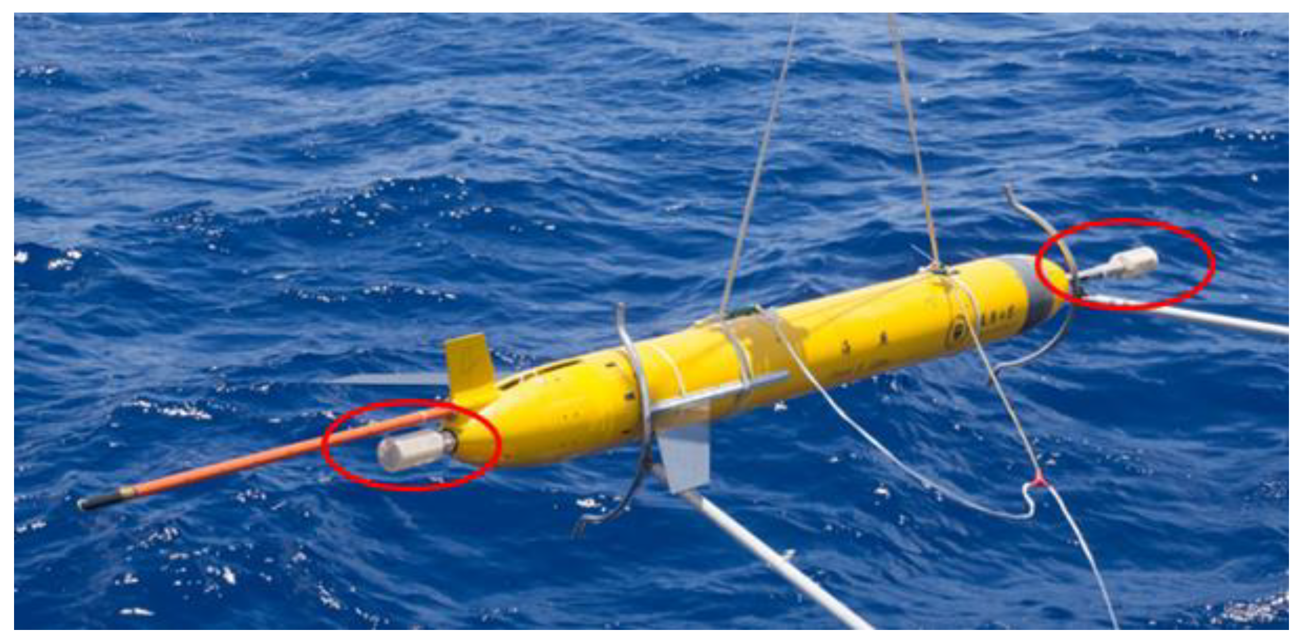
2.1. The Petrel II Glider and the Self-Contained Hydrophones

The Petrel II glider developed by Tianjin University is a buoyancy-driven underwater vehicle. Without a propeller system, the glider travels by changing its buoyancy and the barycenter [17,18,19,20]. The maximum operational depth of Petrel II is 1500 m, and it can navigate by GPS, pressure sensor, compass, and altimeter. The length of the glider is about 2 m and has a weight of 70 kg in the air. The glider communicates through wireless, iridium, and RF modem. The typical cruising speed is 0.5 m/s.

Due to it having no propeller system, the self-noise of the glider is quite low, which makes the Petrel II glider a good platform from which to study underwater acoustics. Figure 1 shows the Petrel II glider in an August 2018 experiment. Two self-contained hydrophones (SCHs) were mounted on the glider to continuously collect the underwater acoustic signal, one at the front and another at the tail. The sample rate of the SCHs is 80 kHz using 24-bit quantization. The SCHs support multiple storage cards of different specifications and can work for several months using lithium batteries.

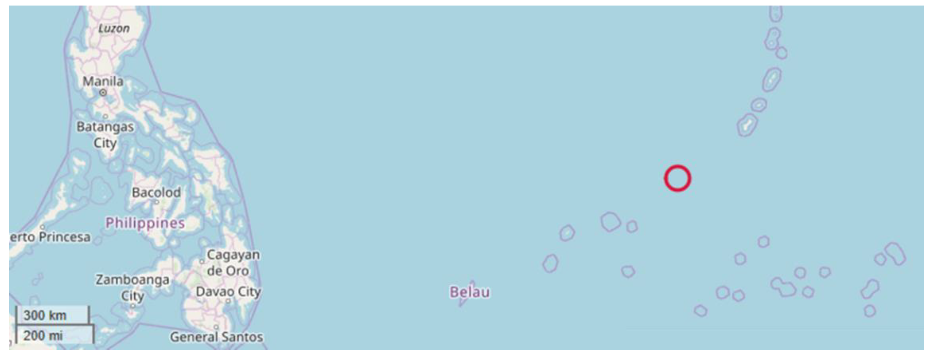
2.2. Experiment Description

In April 2018, a Petrel II glider was deployed in a sea trial near the Mariana Trench. In this experiment, only a single SCH was mounted on the tail of the glider. The total number of dives during the experiment was 32, which took approximately 55 h. The depth of the glider operation ranged from 0 to 800 m. The main purpose of the experiment was to study the characteristics of the self-noise and to preliminarily verify the ability of the glider to serve as a platform to study underwater noise. The location of the experiment is shown in Figure 2.

In August 2018, the second sea trial was held in the South China Sea. The glider was modified to reduce the self-noise and two SCHs were mounted at the front and tail. The total number of dives during the experiment was 31, which took about 92 h. The depth of the glider operation ranged from 0 to 1000 m. The main purpose of the experiment was to verify the underwater signal detection and target azimuth estimation capability of the glider. Two different acoustic sources were deployed and various acoustic signals were transmitted, such as pulse cosine wave (PCW) signals, M-sequence, multitone, and linear frequency-modulated (LFM) signals.

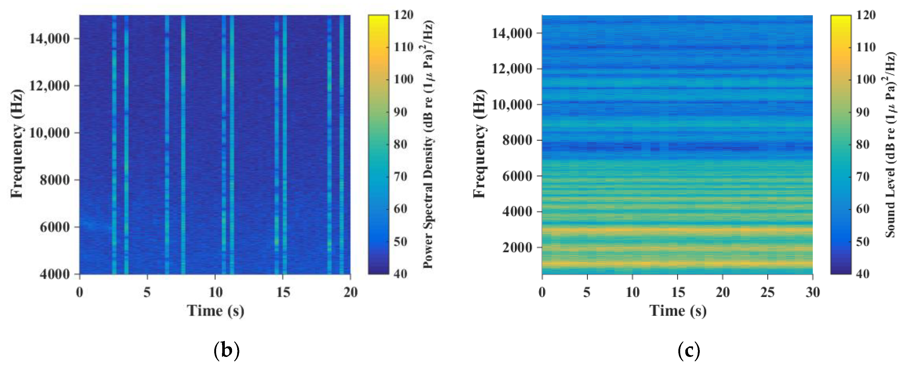
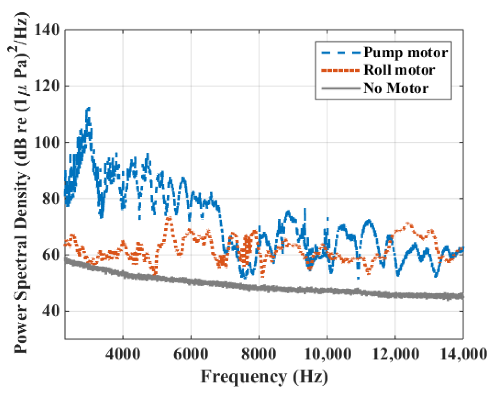
3. Self-Noise of the Petrel II Glider

Before studying the underwater ambient noise and signal detection capability, the self-noise of the Petrel II glider needs to be analyzed. Although the glider has no propeller system, the mechanical structures of the glider for changing the buoyancy and the barycenter still lead to some self-noise. The self-noise mainly comes from two motors in the glider: the pump motor and the roll motor. The function of the pump motor is to change the buoyancy of the glider on the bottom of each dive. The roll motor will work when the glider deviates from the preset direction. It can control the heading by changing the glider’s roll angle. A change of buoyancy also occurs on the surface so the glider can start diving, which is changed by a valve instead of a pump motor.

Figure 3 shows the time and depth of different kinds of self-noise in several dives. The pump motor noise only appeared at the bottom of each dive, and the roll motor noise appeared randomly during each dive.

To illustrate the characteristics of the self-noise in time and frequency, spectrograms of the ambient noise, roll motor noise, and the pump motor noise are displayed in Figure 4. These characteristics are measured during an ordinary dive. As shown in the figure, the ambient noise is relatively flat, the roll motor noise is constructed by broadband pulse signals, and the pump motor noise is constructed by multitone signals. The frequency spectrum of the roll motor noise and the pump motor noise are compared with the noise of no-motor time in Figure 5. The pump motor has the highest noise level and the main energy of the noise is concentrated at 3000–6500 Hz. The roll motor noise level is 10–20 dB higher than the self-noise of no-motor time. As it shows, when no motor works, the noise is quite close to the ambient noise at sea state 3 [22], which means the self-noise of the glider at no-motor time is negligible. However, both motor noises will interfere with the acoustic environment acquisition and signal detection ability of the system. To determine the influence of the motor noise on data acquisition, the proportion of motor occurrence time is estimated using all profile data from two sea trials. The results show that the no-motor time is more than 50% of the total dive time. Furthermore, through trade-offs between course-keeping ability and self-noise reduction, the proportion of no-motor time can be further improved. According to the above analyses, the glider has low self-noise, especially when no motor is working.

In the following, the data when the motor noise occurred will be deleted, so that only motor noise-free data are used.

4. Application of Gliders to Underwater Acoustics

To further illustrate the advantages of the glider for underwater acoustics, in this section, the ambient noises collected at different depths are analyzed first. The underwater passive surveillance ability of the Petrel II glider is then studied from two aspects, the target detection ability and the target azimuth estimation ability, using the data from the sea trial in August 2018.

4.1. Ocean Ambient Noise Acquisition

Since the Petrel II glider travels through the ocean, the ambient noises of different depths can be recorded by SCHs. Figure 6 shows the raw data and the ambient noise level of individual frequencies at different depths from a single profile in April 2018. The peaks in the left figure are caused by the roll motor, and the loud noises on the bottom are caused by the pump motor. After the noise induced by the two motors is removed, the profile data of the ambient noises can be obtained.

As shown in the right-hand panel of Figure 6, the noise level at a higher frequency is lower, which is similar to the results of [22,23]. Moreover, the general trend shows that the ambient noise levels of 2000‒8000 Hz decrease by about 1‒3 dB from 100 m to 700 m during the dive. Since the detection performance is highly correlated to the ambient noise [22,24], the collected ambient noise data can be used as a reference for target detection performance.

4.2. Underwater Passive Surveillance

With SCHs, the Petrel II glider can passively monitor underwater acoustic targets. The data from the sea trial in August 2018 are studied. In the experiment, various acoustic signals were transmitted. Both the multitone signal and the broadband signal are chosen to simulate the unknown target. The transmission loss and the signal direction of arrival (DOA) are estimated, to show the potential of the glider in underwater target detection.

4.2.1. Performance of Signal Receiving

The broadband and multitone signals are used to estimate the transmission loss to illustrate the advantages of the glider in underwater target detection over other autonomous underwater vehicles. Those signals were transmitted by a source installed on the ship, with a frequency ranging from 4000 to 7000 Hz. During the transmission, the ship was continuously drifting on the surface with a speed of around 1 kt. Figure 7 shows the spectrum of the received multitone signal at a certain time, and the frequency range of the signal is 4500–6500 Hz with an interval of 500 Hz. The sound level of the received signal is around 88 dB, so the transmission loss can be estimated by a sonar equation [22]. As shown in Figure 7, the received signal-to-noise ratio (SNR) is higher than 35 dB, which makes it readily detected by the glider.

To obtain the relationship between the transmission loss (TL) and the distance, receptions at different locations were processed. The TL was estimated based on the following sonar equation [22]:

$$\mathrm{TL}=\mathrm{SL}-\mathrm{NL}+\mathrm{DI}-\mathrm{DT},$$

(1)

where SL is the source level, which is known. NL is the noise level, which is estimated using the ambient noise. DI is the receiving directivity index. Since the omnidirectional SCH is used to calculate the results, DI is 0. DT is the received SNR, which can be estimated with NL and the received signal level.

The left-hand panel in Figure 8 is the estimated TL as a function of the range at different frequencies. The theoretical TLs of the cylindrical spreading and spherical spreading with absorption are also compared with the estimated results [22]. As shown in the figure, the trend of TL increases with the distance: the TL of most frequencies is larger than the TL with cylindrical spreading but lower than TL with spherical spreading, and the largest TL is about 74 dB at 5.5 km.

Because of the low noise of the glider, two major factors that affect the ability of target detection are TL and the ambient noise level. However, the detection performance of other AUVs with propeller system will be affected by their self-noise. AUVs are also widely used in underwater surveys [25]. The typical self-noise of AUVs is about 83–116 dB at a frequency range of 4000–7000 Hz [26], which means that the self-noise of the AUV is about 30 dB higher than the ambient noise. However, as for the glider, when there is no motor working, it can receive a signal with the SNR higher than 0 dB as long as the sum of TL and noise level is lower than the source level. Therefore, the SNR of signals received by the AUVs is much lower than that of the glider under the experimental conditions in the paper.

To further expound the advantages of the glider in underwater detection, a simulation is carried out based on the estimated TL from the experiment. In the simulation, the self-noise of the AUV is 83 dB, which is the lowest value in [26]. The source level is set to 130 dB, and the ambient noise level is set to 50 dB, which is a typical value in the frequency band of 4000–7000 Hz, as Figure 6 shows. Both the glider and the AUV are mounted with a single hydrophone, and the signal energy [24,27] is used to detect the source. Assuming the distribution of the amplitude of the noise is Gaussian and the false alarm rate is set to $P_{Fa}={10}^{-2}$, the detection probability $P_D$ can be calculated based on the following equation [24]:

$$P_D=Q_{X_N^2}\left(\frac{Q_{X_N^2}^{-1}\left(P_{Fa}\right)}{SNR+1}\right),$$

(2)

where the $Q_{X_N^2}(\cdot )$ is the chi-square distribution with $N$ degrees of freedom ($N=1$ in the simulation), and $SNR$ is the received signal-to-noise ratio, which can be calculated by the sonar equation. The right-hand panel of Figure 8 shows the simulated detection probability of the glider and the AUV, respectively. As shown in the figure, the detection probability trend of both vehicles decreases with the increase in distance, but in most cases the glider can maintain a detection probability higher than 60% even beyond 5 km. However, the AUV performs poorly when the range is further than 2 km, where most of the detection probability is no more than 20%. This is because the self-noise of AUVs is extremely high, which makes the received SNR much lower compared to the glider under the same conditions. The results of the simulation indicate that the glider performs far better than AUVs with propeller systems in underwater target detection.

4.2.2. Improvement of Signal Receiving Ability via ALE

Although the glider is much quieter than AUVs, the self-noise of the glider, especially the roll motor noise, still has an impact on detection ability. As Figure 3 shows, the roll motor noise appears irregularly and frequently. If the roll motor noise can be eliminated, there will be more time for signal detection and the detection ability can be improved. Thus, to further reduce the influence of the self-noise, the following presents a method using an adaptive filter to improve the performance of signal receiving ability. The ALE is a spectrum estimation technique that is widely used for narrowband signal detection in additive broadband noise [16]. It can suppress broadband signals but enhances narrow band signals. Since the roll motor noise is a broadband signal, it is appropriate to extract the received narrowband signal by the ALE.

As shown in Figure 9, the ALE can be implemented via a least mean squares (LMS) adaptive filter [14]. Different from other adaptive filters, it does not need to know the desired signal. It has two inputs, one of which is the received signal $x\left(n\right)$, which is a combination of the desired narrow band signal $s\left(n\right)$ and noise $w\left(n\right)$. The other input is a delayed version of $x\left(n\right)$, which can be written as $x\left(n-\mathsf{\Delta }\right)$, where $\mathsf{\Delta }$ denotes the delay time.

The first output of the ALE is $y\left(n\right)$, which is the estimation of the desired signal. The second output $e\left(n\right)$ is the difference between the $x\left(n\right)$ and $y\left(n\right)$. In every iteration, ALE separates the narrowband signal and adaptively adjusts its filter weight using the LMS algorithm. The mathematical formulas of ALE are as follows [16]:

$$x\left(n\right)=s\left(n\right)+w\left(n\right)$$

(3)

$$y\left(n\right)={\displaystyle \sum }_{i=1}^L{w}_i\left(n\right)x\left(n-\mathsf{\Delta }-i\right)$$

(4)

$$e\left(n\right)=x\left(n\right)-y\left(n\right)$$

(5)

$$w_i\left(n+1\right)=w_i\left(n\right)+2\mu e\left(n\right)x\left(n-\mathsf{\Delta }-i\right),$$

(6)

where $\mu$ is the step size that controls the convergence rate, and $L$ is the length of the filter.

To illustrate the effectiveness of ALE in a real scenario, a 5 kHz PCW signal received from the experiment in August 2018 was chosen. The spectrogram of the signal is displayed in the left-hand panel of Figure 10. The 5 kHz PCW signal starts at about 30 s, but is corrupted by the roll motor noise. The right-hand panel of Figure 10 is the spectrogram of the ALE’s output signal, where most of the roll motor noise is eliminated, but the PCW signal is enhanced, which makes it much easier to detect than the raw data. Figure 11 shows the spectrum of the raw signal and the ALE output signal. The SNR of the raw 5 kHz PCW signal is no more than 5 dB. However, after it was enhanced by the ALE, the output SNR was not less than 30 dB and the gain of ALE in this scenario was about 25 dB.

Through this algorithm, the detection range of gliders, especially for narrowband signals, can be greatly improved.

4.2.3. Performance of Target Azimuth Estimation

After the target has been detected, the target azimuth is another key parameter in underwater passive surveillance. The azimuth of the target tells the glider which direction the target is in, and location algorithms can be further implemented to locate and track the target [28,29,30].

To test the target azimuth estimation of the Petrel II glider, a source was installed on a ship to transmit various broadband signals every 320 s at 13 m depth. During the transmission, the Petrel II glider was set to travel northward, but, affected by ocean currents, it travelled westward at an average horizontal speed of 0.243 m/s. The maximum depth of the dive was about 500 m. Meanwhile, the ship drifted north at an average speed of 0.566 m/s.

The M-sequence signal is chosen for estimating the azimuth in the paper. It has a frequency band of 4000–7000 Hz with a duration of 12 s. Figure 12 shows the spectrogram and the cross section of the received M-sequence signal. The received signal sound level is about 57 dB in the frequency band and the center frequency is 5.5 kHz.

The signal DOAs are estimated through the time difference of arrival (TDOA) method [10,12]. The TDOA $\mathsf{\Delta }T$ is estimated by calculating the cross-correlation between two SCHs. Due to the good autocorrelation of the broadband signals, the output of the cross-correlation has a sharp peak [31]. The DOA can be calculated based on the following equation:

$$\alpha =\mathrm{acos}\left(\mathsf{\Delta }T{c}_w/d\right),$$

(7)

where $d$ is the distance between two SCHs, $c_w$ is the sound speed in the water, and $\alpha$ is the DOA. Note that $\alpha$ here is in the glider’s “body coordinates.” The altitude of the glider is indispensable when converting the $\alpha$ into global coordinates [12]. Every time a signal is received, the altitude of the Petrel II glider is read from the onboard sensor to calculate the azimuth of the received signal in the global coordinate. If not specifically mentioned, the DOAs in the paper have been converted to global coordinates.

However, when the received SNR is low, the energy of the ambient noise in the low frequencies has a great impact on the estimated results. Thus, only the frequencies in the range of 4000–7000 Hz are utilized to calculate the final results.

The original dead-reckoned locations have large deviations from the actual positions. To get more accurate results, the estimated positions of the glider are calibrated by the depth-averaged current, which can be estimated from the relationship between the dead-reckoned and the actual surface GPS position fix [2]. These positions can be more accurate if a computational model of the ambient currents is used such as the regional ocean modeling system (ROMS) [32], the finite volume coast and ocean model (FVCOM) [33], or the Copernicus marine environment monitoring service (CMEMs) [34]. The depth-averaged current does not reflect the specific information of currents at different depths. However, a computational model can provide vertical and horizontal currents at different depths.

Since only two SCHs are mounted on the glider, the estimated azimuths suffer from port‒starboard ambiguity. Figure 13 shows the diagram of ambiguity, where DOAs are symmetrical to each other with respect to the glider’s heading. In this case, we cannot identify which DOA is formed by the target. In order to distinguish the true DOA, a simple scheme is used. If the glider changes its heading, the image DOA will also change accordingly, but the DOA formed by the true target will remain unchanged. Based on this feature, the true DOA can be easily distinguished.

Figure 14 shows the estimated azimuth results of both sides during the experiment as a function of time. It is obvious that the portside DOAs are more stable. However, the starboard side DOAs shows a strong consistency with glider’s heading. Since the ship’s position will not change to be consistent with the glider’s heading, we can tell that the target has a high probability of being reached in the direction near ${30}^{\circ }$, as can be proven by the ship directions, marked out with dotted lines.

For further explanation, the DOA estimated results at each reception location are plotted in Figure 15. The short green arrows indicate the headings of the glider. The glider was set to travel southward, but, due to the influence of ocean currents, it was pushed westward, which led to an inconsistency in the glider’s headings and its travel direction. The red and blue arrows indicate the estimated azimuths of the port side and starboard side of the glider, respectively.

The ship is in about a ${30}^{\circ }$ direction from the glider, and the effects of the scheme are proven: the port-side DOA results point to the area where the ship is drifting, while the starboard-side DOAs distribute randomly in opposite directions relevant to the glider’s heading. The results indicate that, even if only two SCHs are used, the estimated DOAs can still distinguish the direction of the ship to a certain extent, which shows the potential of the glider to serve as a platform for underwater passive surveillance. If multiple gliders are used to form a sensor network, they can observe a target from different angles to obtain more accurate information. Considering the low energy consumption, low self-noise, and remote control of the glider, it can be easily redeployed to a new area, bringing about more advantages for long-term underwater network sensing.

5. Conclusions

This paper illustrates the application of the Petrel II glider to underwater acoustics by sea trials. First, the self-noise of the glider was studied to show the ability of the glider to serve as an underwater acoustic sensing platform. Both the spectrogram and spectrum of different kinds of self-noise were displayed and compared with the ambient noise. The results showed the quietness of the Petrel II glider. Then, the applications of gliders in underwater acoustics were analyzed from two aspects: ocean ambient noise acquisition and underwater passive surveillance. Since the self-noise of the glider appeared intermittently, the ambient noise could be recorded during the no-motor noise time. By estimating the transmission loss using transmitted signals, the signal receiving ability of the Petrel II glider was discussed. Meanwhile, a simulation of target detection probability was carried out, and the results indicated that the glider had a great advantage over other underwater vehicles with propeller systems. Moreover, in order to reduce the influence of self-noise, an adaptive line enhancement algorithm was introduced and tested using experimental data.

Because the glider had two SCHs at both ends, the target azimuth estimation ability was analyzed using the broadband signals transmitted by a drifting ship, and a simple scheme to distinguish the true DOA from the port‒starboard ambiguity was illustrated. Two SCHs formed a simple linear array with a large aperture, through which the glider could locate an unknown target. The array also had lower energy consumption compared with other linear arrays with more elements. Moreover, this installation reduced the impact of the self-noise because the two SCHs were as far away from the glider as possible. Furthermore, the glider can improve the signal receiving ability through array signal processing technology such as beamforming. To make the scheme more reliable, the law of heading changes should be designed carefully, and the balance of energy consumption and azimuth estimation ability needs to be considered.

References

1. Rudnick, D.L.; Davis, R.E.; Eriksen, C.C.; Fratantoni, D.M.; Perry, M.J. Underwater gliders for ocean research. Mar. Technol. Soc. J. 2004, 38, 73–84. [Google Scholar] [CrossRef]
2. Rudnick, D.L. Ocean research enabled by underwater gliders. Annu. Rev. Mar. Sci. 2016, 8, 519–541. [Google Scholar] [CrossRef] [PubMed]
3. Nichols, B.; Sabra, K.G. Cross-Coherent vector sensor processing for spatially distributed glider networks. J. Acoust. Soc. Am. 2015, 138, EL329–EL335. [Google Scholar] [CrossRef] [PubMed]
4. Meyer, D. Glider technology for ocean observations: A review. Ocean Sci. Discuss. 2016, 2016, 1–26. [Google Scholar] [CrossRef]
5. Rogers, E.O.; Genderson, J.G.; Smith, W.S.; Denny, G.F.; Farley, P.J. Underwater acoustic glider. In Proceedings of the 2004 IEEE International Geoscience and Remote Sensing Symposium, Anchorage, AK, USA, 20–24 September 2004; pp. 2241–2244. [Google Scholar]
6. Maguer, A.; Dymond, R.; Grati, A.; Stoner, R.; Guerrini, P.; Troiano, L.; Alvarez, A. Ocean gliders payloads for persistent maritime surveillance and monitoring. In Proceedings of the 2013 IEEE OCEANS, San Diego, CA, USA, 23–27 September 2013; pp. 1–8. [Google Scholar]
7. Baumgartner, M.F.; Van Parijs, S.M.; Wenzel, F.W.; Tremblay, C.J.; Carter Esch, H.; Warde, A.M. Low frequency vocalizations attributed to sei whales (balaenoptera borealis). J. Acoust. Soc. Am. 2008, 124, 1339–1349. [Google Scholar] [CrossRef] [PubMed]
8. Baumgartner, M.F.; Fratantoni, D.M.; Hurst, T.P.; Brown, M.W.; Cole, T.V.; Van Parijs, S.M.; Johnson, M. Real-time reporting of baleen whale passive acoustic detections from ocean gliders. J. Acoust. Soc. Am. 2013, 134, 1814–1823. [Google Scholar] [CrossRef] [PubMed]
9. Wall, C.C.; Lembke, C.; Mann, D.A. Shelf-scale mapping of sound production by fishes in the eastern Gulf of Mexico, using autonomous glider technology. Mar. Ecol. Prog. Ser. 2012, 449, 55–64. [Google Scholar] [CrossRef]
10. Küsel, E.T.; Munoz, T.; Siderius, M.; Mellinger, D.K.; Heimlich, S.L. Marine mammal tracks from two-hydrophone acoustic recordings made with a glider. Ocean Sci. 2017, 13, 273–288. [Google Scholar] [CrossRef]
11. Dassatti, A.; Van der Schaar, M.; Guerrini, P.; Zaugg, S.; Houégnigan, L.; Maguer, A.; Andre, M. On-board underwater glider real-time acoustic environment sensing. In Proceedings of the 2011 IEEE OCEANS, Santander, Spain, 6–9 June 2011; pp. 1–8. [Google Scholar]
12. Tesei, A.; Been, R.; Williams, D.; Cardeira, B.; Galletti, D.; Cecchi, D.; Maguer, A. Passive acoustic surveillance of surface vessels using tridimensional array on an underwater glider. In Proceedings of the 2015 IEEE OCEANS, Genoa, Italy, 18–21 May 2015; pp. 1–8. [Google Scholar]
13. Cazau, D.; Bonnel, J.; Jouma’a, J.; Le Bras, Y.; Guinet, C. Measuring the marine soundscape of the Indian Ocean with southern elephant seals used as acoustic gliders of opportunity. J. Atmos. Ocean. Technol. 2017, 34, 207–223. [Google Scholar] [CrossRef]
14. Bershad, N.; Feintuch, P.; Reed, F.; Fisher, B. Tracking characteristics of the LMS adaptive line enhancer-response to a linear chirp signal in noise. IEEE Trans. Acoust. Speech Signal Process 1980, 28, 504–516. [Google Scholar] [CrossRef]
15. Cho, N.I.; Choi, C.H.; Lee, S.U. Adaptive line enhancement by using an IIR lattice notch filter. IEEE Trans. Acoust. Speech Signal Process 1989, 37, 585–589. [Google Scholar]
16. Ghogho, M.; Ibnkahla, M.; Bershad, N.J. Analytic behavior of the LMS adaptive line enhancer for sinusoids corrupted by multiplicative and additive noise. IEEE Trans. Signal Process 1998, 46, 2386–2393. [Google Scholar] [CrossRef]
17. Liu, L.; Xiao, L.; Lan, S.Q.; Liu, T.T.; Song, G.L. Using Petrel II Glider to analyze underwater noise spectrogram in the South China Sea. Acoust. Aust. 2018, 46, 151–158. [Google Scholar] [CrossRef]
18. Liu, F.; Wang, Y.; Wang, S. Development of the hybrid underwater glider Petrel-II. Sea Technol. 2014, 55, 51–54. [Google Scholar]
19. Liu, F.; Wang, Y.H.; Wu, Z.L.; Wang, S.X. Motion analysis and trials of the deep sea hybrid underwater glider Petrel-II. China Ocean Eng. 2017, 31, 55–62. [Google Scholar] [CrossRef]
20. Yu, J.C.; Zhang, A.Q.; Jin, W.M.; Chen, Q.; Tian, Y.; Liu, C.J. Development and experiments of the sea-wing underwater glider. China Ocean Eng. 2011, 25, 721–736. [Google Scholar] [CrossRef]
21. OpenStreetMap. Available online: https://www.openstreetmap.org/copyright (accessed on 23 October 2019).
22. Kinsler, L.E.; Frey, A.R.; Mayer, W.G. Fundamentals of Acoustics, 4th ed.; Wiley-VCH: Weinheim, Germany, 1999; pp. 450–452. [Google Scholar]
23. Shooter, J.A.; DeMary, T.E.; Wittenborn, A.F. Depth dependence of noise resulting from ship traffic and wind. IEEE J. Oceanic Eng. 1990, 15, 292–298. [Google Scholar] [CrossRef]
24. Kay, S. Fundamentals of Statistical Signal Processing, Volume 2: Detection Theory; Prentice Education: Cranbury, NJ, USA, 1998; pp. 465–466. [Google Scholar]
25. Hwang, J.; Bose, N.; Fan, S. AUV Adaptive Sampling Methods: A Review. Appl. Sci. 2019, 9, 3145. [Google Scholar] [CrossRef]
26. Holmes, J.D.; Carey, W.M.; Lynch, J.F. An overview of unmanned underwater vehicle noise in the low to mid frequency bands. J. Acoust. Soc. Am. 2010, 127, 1812. [Google Scholar] [CrossRef]
27. Goldhahn, R.; Braca, P.; LePage, K.D.; Willett, P.; Marano, S.; Matta, V. Environmentally sensitive particle filter tracking in multistatic AUV networks with port-starboard ambiguity. In Proceedings of the 2014 IEEE International Conference on Acoustics, Speech and Signal Processing, Florence, Italy, 4–9 May 2014; pp. 1458–1462. [Google Scholar]
28. Jiang, C.; Li, J.; Xu, W. Joint Detection and Tracking via Path Planning in the Mobile Underwater Sensing Network. In Proceedings of the 2018 IEEE 10th International Conference on Wireless Communications and Signal Processing, Hangzhou, China, 18–20 October 2018; pp. 1–6. [Google Scholar]
29. Chen, Z.; Xu, W. Joint Passive Detection and Tracking of Underwater Acoustic Target by Beamforming-Based Bernoulli Filter with Multiple Arrays. Sensors 2018, 18, 4022. [Google Scholar] [CrossRef] [PubMed]
30. Luo, J.; Han, Y.; Fan, L. Underwater acoustic target tracking: A review. Sensors 2018, 18, 112. [Google Scholar] [CrossRef] [PubMed]
31. Hassab, J.; Boucher, R. Optimum estimation of time delay by a generalized correlator. IEEE Trans. Acoust. Speech Signal Process 1979, 27, 373–380. [Google Scholar] [CrossRef]
32. Shchepetkin, A.F.; McWilliams, J.C. The regional oceanic modeling system (ROMS): A split-explicit, free-surface, topography-following-coordinate oceanic model. Ocean Model. 2005, 9, 347–404. [Google Scholar] [CrossRef]
33. Chen, C.; Liu, H.; Beardsley, R.C. An unstructured grid, finite-volume, three-dimensional, primitive equations ocean model: application to coastal ocean and estuaries. J. Atmos. Ocean. Technol. 2003, 20, 159–186. [Google Scholar] [CrossRef]
34. Copernicus Marine Environment Monitoring Service. Available online: http://marine.copernicus.eu/ (accessed on 23 October 2019).
Figure 1. The “Petrel II” glider in the August 2018 experiment. Two SCHs are indicated by red circles, one at the front of the glider and the other at the tail.
Applsci 09 04839 g001
Figure 2. The location of the experiment in April 2018 is marked with a red circle on the map. Map data: © OpenStreetMap contributors, CC BY-SA [21].
Applsci 09 04839 g002
Figure 3. The occurrences of different self-noise as a function of time and depth. The blue line indicates the dive profiles of the glider. The yellow dots and red asterisks correspond to the operation time and depth of the roll motor and pump motor, respectively. The roll motor works intermittently, while the pump motor only works in the bottom region of each dive. Measured by statistical data, the no-motor time is more than 50% of the total dive time.
Applsci 09 04839 g003
Figure 4. The spectrograms of the ambient noise (a), roll motor noise (b) and the pump motor noise (c), respectively. The ambient noise is relatively flat. The noise of the roll motor is a broadband pulse signal, and the pump motor is a multitone signal.
Applsci 09 04839 g004aApplsci 09 04839 g004b
Figure 5. The frequency spectra of the roll motor noise and the pump motor noise compared with the noise of no-motor time, respectively. The pump motor noise has the highest noise level, and the roll motor noise level is 10‒20 dB higher than that of the no-motor time. The noise at no-motor time is quite closed to the ambient noise at sea state 3 [22].
Applsci 09 04839 g005
Figure 6. The raw data (a) and the ambient noises (b) of individual frequencies from a single profile in April 2018.
Applsci 09 04839 g006
Figure 7. The spectrum of the received multitone signal. The frequency range of the transmitted signal is 4500–6500 Hz.
Applsci 09 04839 g007
Figure 8. The estimated transmission losses of different frequencies at different ranges (a) using both broadband and multitone signals, and the simulated detection probability (b). The dashed line represents the theoretical transmission loss of cylindrical spreading and the dotted line represents the spherical spreading. The red plus sign and blue triangle in the right-hand panel represent the detection probability of the glider and the simulated AUV with self-noise of 83 dB, respectively.
Applsci 09 04839 g008
Figure 9. The block diagram of the ALE.
Applsci 09 04839 g009
Figure 10. The spectrograms of raw data (a) and the ALE filtered data (b), respectively. The signal starts in about 30 s.
Applsci 09 04839 g010
Figure 11. The spectrum of raw data and the ALE filtered data, respectively.
Applsci 09 04839 g011
Figure 12. The spectrogram (a) and one example cross section (b) of the received broadband signal. The signal frequency band is 4‒7 kHz.
Applsci 09 04839 g012
Figure 13. The diagram of ambiguity. Two circles indicate SCHs mounted on the glider. Port- and starboard-side DOAs are symmetrical to each other with respect to the glider’s heading. If the glider changes its heading, the image DOA will also change. However, the DOA formed by the true target remains unchanged.
Applsci 09 04839 g013
Figure 14. Estimated DOAs of both sides as a function of time. The yellow line is the heading of the glider, while the dotted line with diamonds is the ship’s direction. The starboard DOAs and the heading have a similar transformation pattern, because the starboard DOAs are not true azimuths of the target but mirror angles of the azimuths.
Applsci 09 04839 g014
Figure 15. The sea trial scenario with the estimate DOAs (a) and the local enlargement of the black dotted bordered rectangle (b). The black line is the path of the glider, and the blue circles are the positions of each signal reception. The yellow line with dots is the path of the ship, and the drift direction of the ship is also marked. The glider started diving from the square and ended at the red asterisk. The red and blue arrows represent the estimated DOAs in the port and starboard sides of the glider, respectively. The short green arrows represent the headings of the glider at each signal reception time. The glider was set to travel southward, but due to the influence of ocean currents, the heading of the glider is not consistent with the travel direction.
Applsci 09 04839 g015