Revisiting the Meandering Instability During Step-Flow Epitaxy

Department of Mathematics and Computer Science, Auburn University at Montgomery, Montgomery, AL 36117, USA
Appl. Sci. 2019, 9(22), 4840; https://doi.org/10.3390/app9224840
Submission received: 9 September 2019
/
Revised: 21 October 2019
/
Accepted: 7 November 2019
/
Published: 12 November 2019
(This article belongs to the Section Materials Science and Engineering)
Abstract
:This paper starts with a generalized Burton, Cabrera and Frank (BCF) model by considering the energetic contribution of the adjacent terraces to the step chemical potential. We use the linear stability analysis of the quasistatic free-boundary problem for a two-dimensional step separated by broad terraces to study the step-meandering instabilities. The results show that the equilibrium adatom coverage has influence on the morphological instabilities.
1. Introduction
For molecular-beam epitaxy (MBE), it is well accepted that the thin-film epitaxial growth on a vicinal surface via step flow at a sufficient high temperature constitutes an ideal growth regime [1,2]. The overview and discussion of the crystal growth can be found in References [2,3,4,5,6]. In the step-flow regime, the temperature, while below the surface roughening temperature, is sufficiently high to make adatom diffusion fast and, concomitantly, island nucleation improbable. Thus, the sole mechanism for growth or sublimation is the attachment of adatoms to, or their detachment from, the pre-existing steps. Specifically, during the growth on a surface consisting of terraces separated by steps, the deposited atoms diffuse across the terraces and attach to the step, diffuse along the edge and eventually incorporate into the crystalline bulk (Figure 1).
Therefore, it is important to study the morphological instability of the terrace edge. Reference [7] showed a scanning tunneling microscopy image of a Si(001) surface which consists of broad terraces separated by steps of atomic height. The experimental and theoretical efforts have been worked on the one-dimensional structures, such as quantum wires, as the result of morphological instability during the epitaxy of self-assembling materials [5]. A step-flow model for the heteroepitaxy of a generic, strained, substitutional, binary alloy has been studied [8]. References [9,10,11] have investigated modeling epitaxial growth by kinetic Monte Carlo simulations. Some applications and experiments concerning epitaxy in thin films have been developed [12,13,14].
In 1951, Burton, Cabrera and Frank (BCF) [15] developed a model for the growth of crystals and described the crystal growth as a regular flow of edges. In the presence of the Ehrlich–Schwoebel barrier, the meandering of the periodic monatomic steps separated by broad terraces has been discussed in Reference [16]. The classical BCF model, however, does not consider the energetic contribution of the adjacent terraces to the step chemical potential and hence cannot explain some phenomena observed experimentally [5]. Therefore, the classical BCF framework was extended by considering this energetic contribution in Reference [17] which developed a thermodynamically consistent continuum theory for the step-flow epitaxy of single-component crystalline films and studied the step-bunching instabilities of one-dimensional step-flow epitaxy. Since the general theory is two-dimensional, it is appropriate to investigate the step-meandering instabilities of a two-dimensional single step separated by broad terraces. We discuss the details in Section 2.
The generalized BCF model in Reference [17] can be described by the following free-boundary problem that consists of the reaction-diffusion equation on the upper and lower terraces
with the step-edge boundary conditions
and the step evolution equation
Here is the terrace adatom density; is the adatom chemical potential; M is the atomic mobility; F is the deposition flux; is the desorption coefficient; n is the unit normal to the step pointing to the lower terrace; is the normal derivative of the step chemical potential; is the step chemical potential; is the bulk atomic density; a is the step height; V is the velocity of the step; () is the kinetic coefficient for the attachment-detachment of adatoms from the lower (upper) terrace onto the step edge; and and represent the limiting value when approaching the step from the lower and upper terraces respectively.
In this paper, we consider a general step chemical potential derived in Reference [18]
where is the (nominal) crystalline chemical potential; and are the stiffness and curvature of the step respectively; and is the the jump in the terrace grand canonical potential across the step which represents the energy contribution of the adjacent terraces to the step chemical potential. When the time scale for the step migration is large compared to the time scale for the adatom diffusion on the terraces, the reaction-diffusion Equation (1) is approximated by the corresponding steady-state counterpart on the terraces
and the step-edge boundary conditions (2) are replaced by
Hence the step evolution Equation (3) can be formulated as
In the next section, we will discuss the meandering instabilities of the two-dimensional step separated by broad terraces for the free boundary problem consisting of (5)–(7).
2. Stability Analysis
In this paper, we employ a linear stability analysis to study step-meandering. For our convenience, let . The steady-state reaction-diffusion Equation (5) becomes the Helmholtz equation
where is the surface diffusion length. We introduce a constant parameter and a dimensionless parameter , the equilibrium adatom coverage, which measures the equilibrium adatom density relative to the bulk atomic density . For the adatom grand canonical potential in (4), we adopt the linear approximation with a positive constant in [17]. Therefore, the step-edge boundary conditions (6) can be written as
where . And the evolution equation for u is
with .
The general solution to the Helmholtz Equation (8) is given by the form of
where . Assume there is a small amplitude sinusoid perturbation with a wave vector k for the step. Then the position of the step is given by
Therefore the curvature and the normal vector . If we allow the accuracy of the solution u up to the first order in , the solution will be in the form of
where is the solution appropriate for perfectly straight steps, that is, is allowed in (11).
To compute the velocity of the step, we take the time derivative of (12) and get
On the other hand, we can also use (10) to compute the velocity. Later we can see it has the form of
where the stability function with certain functions f and g. Equations (14) and (15) imply . It shows that the sign of determines the growth or decay of perturbation.
It is necessary to define the kinetic coefficients for the attachment-detachment of adatoms from the lower and upper terrace onto the step edge and a surface capillary length . These notations will be used in the following section.
2.1. The Dependence of the Stability Function
Now we consider the general situation that the kinetic coefficients for the attachment-detachment of adatoms from the lower and upper terrace onto the step edge are finite, that is, are finite.
To find the solution u in the form of (13), we first need to obtain for the case of perfectly straight steps where the curvature and the normal vector . Notice that
Consequently, the boundary condition (9) for the straight step case becomes
A and B in can be solved from the linear system (16). Now we allow the accuracy up to the first order of .
We have and . Then the first-order Taylor expansion about gives that
Substituting (17) into the boundary condition (9) and equating the like powers of show that, for the first order in , we have
The coefficients and can be solved from the linear system (18). Therefore, we obtain the solution u in the form of (13). Substituting u into (10), we can compute the velocity V of a single step in the form of
Here
and
which is in the form of . From the straight forward calculation, we can get
and
where
It is known that the energy contribution of the adjacent terraces to the step chemical potential is significant if the equilibrium adatom density has the same magnitude as the bulk atomic density [19]. It is interesting to see how the equilibrium adatom coverage affects the step-meandering instability. The behavior of the stability function for different is illustrated in Figure 2 with some reasonable parameter values. If is positive, the perturbation grows. If is negative, the perturbation decays. As increases, the critical value of k such that moves to the left.
Next we want to discuss the analytic expressions for this critical value . Consider the special case of upper terrace blocking (). Then
and
Therefore, , that is, gives that
The analytic expressions for can be obtained from (26) in the limiting cases of very large and very small terrace widths.
When , we have
where is the surface capillary length. Since is real, the prerequisite for morphological instability is . Figure 3 illustrates the dependence of on the cutoff for different values of .
When (and , the critical wavelength ),
The cutoff here is .
Remark 1.
By using a similar method, we can compute for the limiting situation where the step attachment is infinitely fast from the lower terrace and infinitely slow from the upper terrace (). We can show that
and
which is in the form of . From the straight forward calculation, we obtain
and
Notice that implies that . Hence is positive. Since , it also implies is positive. As for the critical value , when , we find
Since is real, we have a prerequisite for morphological instability . when (and ), we find
Now the cutoff of ξ is .
2.2. The Dependence of the Critical Capillary Length
We also observe that there is a critical value of so that the morphologically stable step flow occurs if and the morphologically unstable step flow occurs if . In order to investigate , we expand to get the critical value for small and real k. The following expansions are needed during the calculation:
Expand the equation up to by (35) with and given by (21) and (22). Then solving for gives the critical value
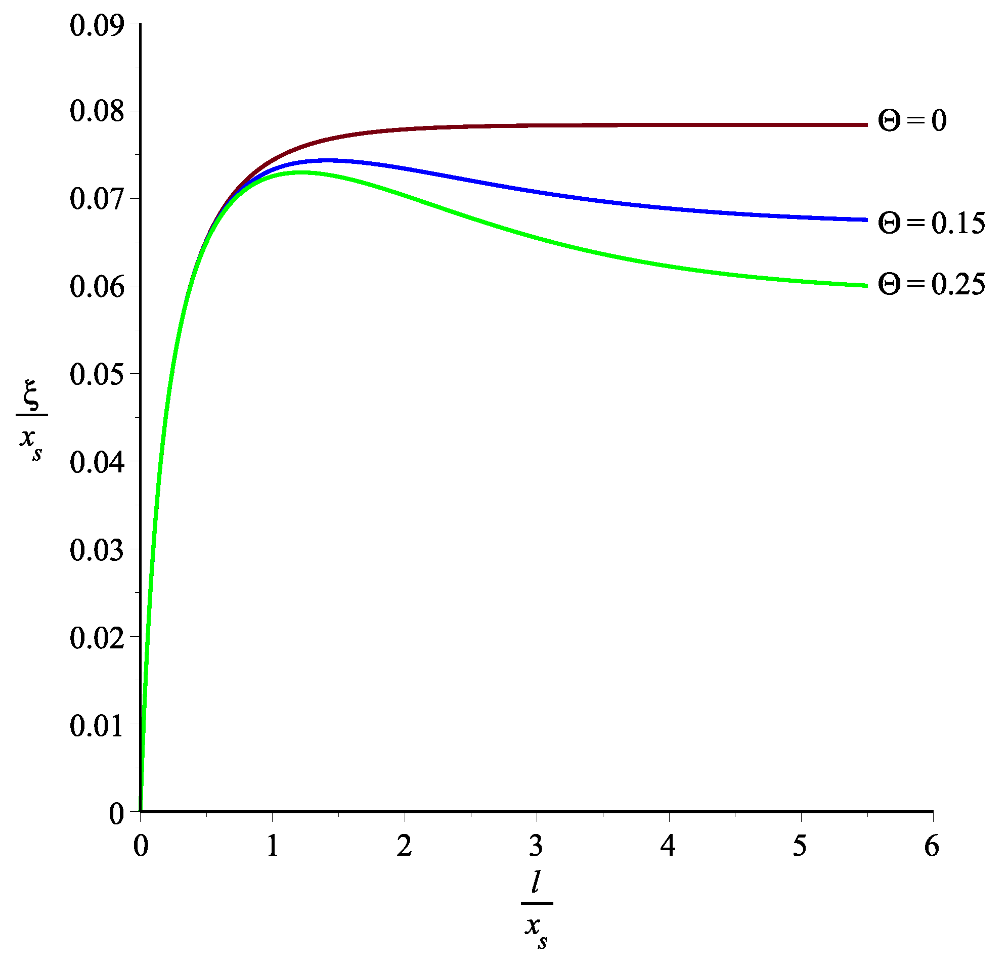
If , then the perturbation decays. If , then the perturbation grows. The expression of in (36) exhibits the dependence. The graph of for different is shown in Figure 4. It can be seen that the curve moves downward as increases.
3. Conclusions
We started with a generalized BCF model by considering the energetic contribution of the adjacent terraces to the step chemical potential and discussed the step-meandering instabilities of the two-dimensional step separated by broad terraces. Our results show that the single-component crystal growth on a vicinal surface can pass from stable to unstable status. We can also see how the equilibrium adatom coverage affects the instabilities of the step meandering. It shows that the increase of can stabilize the step meandering. In the near future, the step-bunching instabilities of a two-dimensional periodic train of steps will be investigated.
Funding
This research received no external funding.
Acknowledgments
Thanks Michel E. Jabbour for his extremely valuable discussion and advising.
Conflicts of Interest
The authors declare no conflict of interest.
References
- Rosenberger, F. Crystal Growth Kinetics. In Interfacial Aspects of Phase Transformations; Mutaftschiev, B., Ed.; Reidel: Dordrecht, Holland, 1982; pp. 315–364. [Google Scholar]
- Tsao, J.F. Materials Fundamentals of Molecular Beam Epitaxy; Academic Press: New York, NY, USA, 1993. [Google Scholar]
- Saito, Y. Statistical Physics of Crystal Growth; World Scientific: Singapore, 1996. [Google Scholar]
- Pimpinelli, A.; Villain, J. Physics of Crystal Growth; Cambridge University Press: Cambridge, UK, 1998. [Google Scholar]
- Krug, J. Multiscale Modeling in Epitaxial Growth; Voigt, A., Ed.; Birkhauser: Berlin, Germany, 2005; Chapter 2; pp. 69–95. [Google Scholar]
- Jeong, H.C.; Williams, E.D. Steps on Surfaces: Experiment and Theory. Surf. Sci. Rep. 1999, 34, 171–294. [Google Scholar] [CrossRef]
- Haußer, F.; Otto, F.; Penzler, P.; Voigt, A. Numerical Methods for the Simulation of Epitaxial Growth and Their Application in the Study of a Meander Instability. In Mathematics—Key Technology for the Future; Krebs, H.J., Jäger, W., Eds.; Springer: Berlin/Heidelberg, Germany, 2008. [Google Scholar]
- Haußer, F.; Jabbour, M.E.; Voigt, A. A Step-Flow Model for the Heteroepitaxial Growth of Strained, Substitutional, Binary Alloy Films with Phase Segregation: I. Theory. Multiscale Model. Simul. 2007, 6, 158–189. [Google Scholar] [CrossRef]
- Pimpinelli, A.; Videcoq, A.; Vladimirova, M. Kinetic surface patterning in two-particle models of epitaxial growth. Appl. Surf. Sci. 2001, 175–176, 55–61. [Google Scholar] [CrossRef]
- DeVita, J.P.; Sander, L.M.; Smereka, P. Multiscale kinetic Monte Carlo algorithm for simulating epitaxial growth. Phys. Rev. B 2005, 72, 205421. [Google Scholar] [CrossRef]
- Hamouda, A.B.; Pimpinelli, A.; Phaneuf, R.J. Anomalous scaling in epitaxial growth on vicinal surfaces: Meandering and mounding instabilities in a linear growth equation with spatiotemporally correlated noise. Surf. Sci. 2008, 602, 2819–2827. [Google Scholar] [CrossRef]
- Bean, J.C. Strained-Layer Epitaxy of Germanium-Silicon Alloys. Science 1985, 230, 127–131. [Google Scholar] [CrossRef] [PubMed]
- Wagner, S.; Klose, P.; Burlaka, V.; Nörthemann, K.; Hamm, M.; Pundt, A. Structural Phase Transitions in Niobium Hydrogen Thin Films: Mechanical Stress, Phase Equilibria and Critical Temperatures. ChemPhysChem 2019, 20, 1890–1904. [Google Scholar] [CrossRef] [PubMed]
- Eliseev, E.A.; Morozovska, A.N.; Nelson, C.T.; Kalinin, S.V. Intrinsic structural instabilities of domain walls driven by gradient coupling: Meandering antiferrodistortive-ferroelectric domain walls in BiFeO3. Phys. Rev. B 2019, 99, 014112. [Google Scholar] [CrossRef]
- Burton, W.K.; Cabrera, N.; Frank, F.C. The growth of crystals and the equilibrium structure of their surfaces. Phil. Trans. R. Soc. Lond. A 1951, 243, 299–358. [Google Scholar] [CrossRef]
- Bales, G.S.; Zangwill, A. Morphological instability of a terrace edge during step-flow growth. Phys. Rev. B 1990, 41, 5500–5508. [Google Scholar] [CrossRef] [PubMed]
- Cermelli, P.; Jabbour, M.E. Possible mechanism for the onset of step-bunching instabilities during the epitaxy of single-species crystalline films. Phys. Rev. B 2007, 75, 165409. [Google Scholar] [CrossRef]
- Cermelli, P.; Jabbour, M.E. Multispecies epitaxial growth on vicinal surfaces with chemical reactions and diffusion. Proc. Roy. Soc. A 2005, 461, 3483–3504. [Google Scholar] [CrossRef]
- Tersoff, J.; Johnson, M.D.; Orr, B.G. Adatom Densities on GaAs: Evidence for Near-Equilibrium Growth. Phys. Rev. Lett. 1997, 78, 282. [Google Scholar] [CrossRef]
Figure 1.
Schematic view of the steps separated by broad terraces with mean width l on which the deposited adatoms diffuse across the terraces and attach to the step, diffuse along the edge and eventually incorporate into the crystalline bulk.
Figure 1.
Schematic view of the steps separated by broad terraces with mean width l on which the deposited adatoms diffuse across the terraces and attach to the step, diffuse along the edge and eventually incorporate into the crystalline bulk.

Figure 2.
The stability function for . Here we take , , , , .

Figure 3.
The variation of the cutoff versus for various values of .
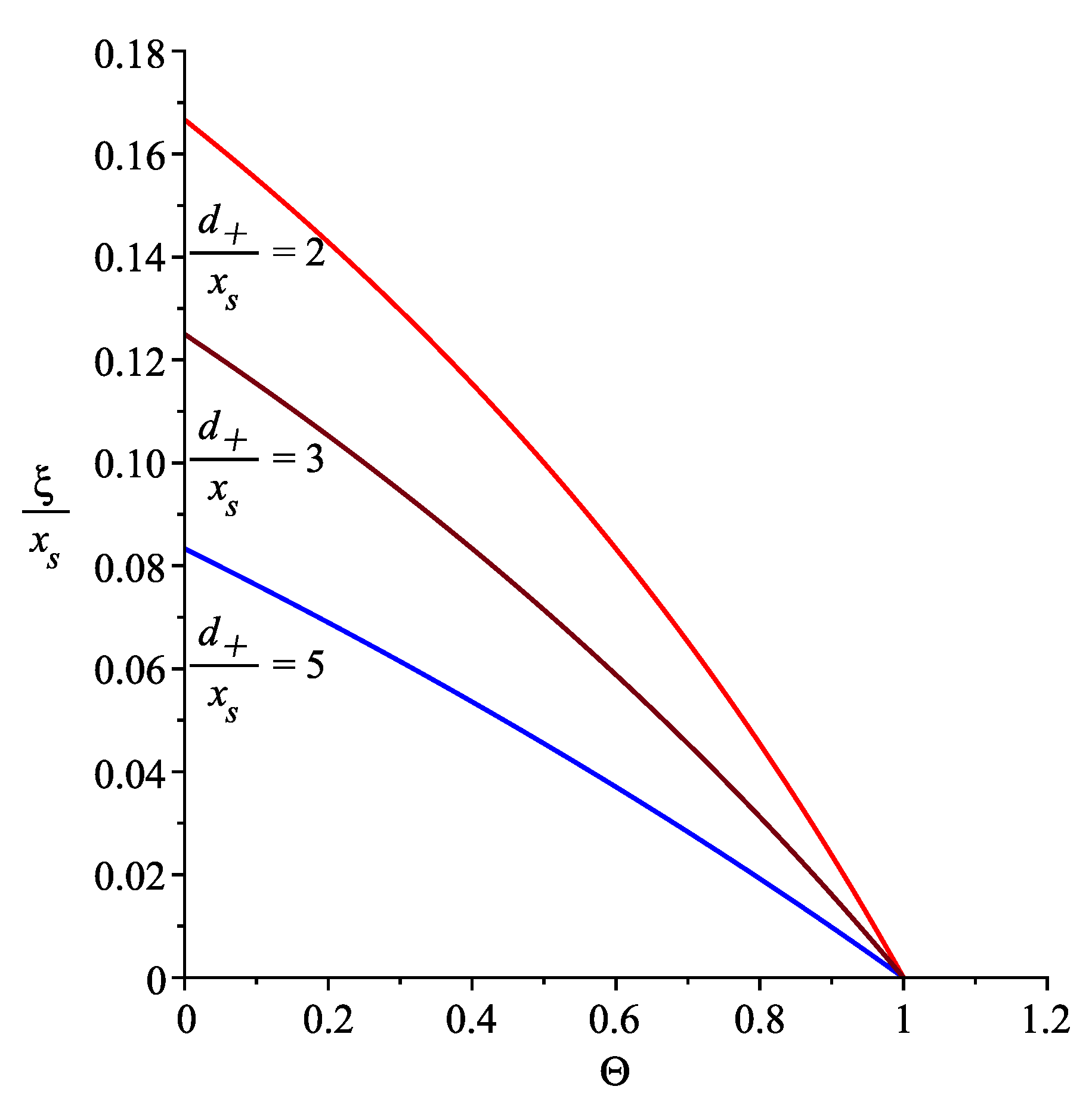
Figure 4.
The critical value for . Here we take , . When , the perturbation decays. When , morphologically unstable step flow occurs.
Figure 4.
The critical value for . Here we take , . When , the perturbation decays. When , morphologically unstable step flow occurs.
© 2019 by the author. Licensee MDPI, Basel, Switzerland. This article is an open access article distributed under the terms and conditions of the Creative Commons Attribution (CC BY) license (http://creativecommons.org/licenses/by/4.0/).
Share and Cite
MDPI and ACS Style
Chen, Y. Revisiting the Meandering Instability During Step-Flow Epitaxy. Appl. Sci. 2019, 9, 4840. https://doi.org/10.3390/app9224840
AMA Style
Chen Y. Revisiting the Meandering Instability During Step-Flow Epitaxy. Applied Sciences. 2019; 9(22):4840. https://doi.org/10.3390/app9224840
Chicago/Turabian StyleChen, Yue. 2019. "Revisiting the Meandering Instability During Step-Flow Epitaxy" Applied Sciences 9, no. 22: 4840. https://doi.org/10.3390/app9224840
Note that from the first issue of 2016, this journal uses article numbers instead of page numbers. See further details here.