Flexible-Link Multibody System Eigenvalue Analysis Parameterized with Respect to Rigid-Body Motion

Abstract

The dynamics of flexible multibody systems (FMBSs) is governed by ordinary differential equations or differential-algebraic equations, depending on the modeling approach chosen. In both the cases, the resulting models are highly nonlinear. Thus, they are not directly suitable for the application of the modal analysis and the development of modal models, which are very useful for several advanced engineering techniques (e.g., motion planning, control, and stability analysis of flexible multibody systems). To define and solve an eigenvalue problem for FMBSs, the system dynamics has to be linearized about a selected configuration. However, as modal parameters vary nonlinearly with the system configuration, they should be recomputed for each change of the operating point. This procedure is computationally demanding. Additionally, it does not provide any numerical or analytical correlation between the eigenpairs computed in the different operating points. This paper discusses a parametric modal analysis approach for FMBSs, which allows to derive an analytical polynomial expression for the eigenpairs as function of the system configuration, by solving a single eigenvalue problem and using only matrix operations. The availability of a similar modal model, which explicitly depends on the system configuration, can be very helpful for, e.g., model-based motion planning and control strategies towards to zero residual vibration employing the system modal characteristics. Moreover, it allows for an easy sensitivity analysis of modal characteristics to parameter uncertainties. After the theoretical development, the method is applied and validated on a flexible multibody system, specifically using the Equivalent Rigid Link System dynamic formulation. Finally, numerical results are presented and discussed.

1. Introduction

The dynamic behavior of a mechanical system can be easily studied by means of modal analysis, which provides the system modal parameters or characteristics (i.e., natural frequencies, mode shapes, and damping ratios). The knowledge of the modal characteristics is a fundamental requirement for the implementation of several advanced model-based engineering techniques, such as motion planning [1], control design [2,3], stability analysis [4,5], model reduction [6,7,8,9,10], model updating [11,12,13], and structural modification [14,15,16].

Modal analysis relies on the solution of an eigenvalue problem, which seeks the eigenvalues and eigenvectors associated to a linear system of equations. However, the adoption of such an analysis may provide a useful insight also for the study of mechanical systems whose dynamics is not governed by linear time-invariant equations. A significant class of mechanical systems that falls in this folder is the one of the flexible-link multibody systems (FMBSs). Such systems are robots or mechanisms that can deflect due to external loads or internal body forces, whose motion is described by means of kineto-elastodynamic models, hereafter referred to as dynamic models [17]. Several contributions can be found in the literature on the modeling of such systems as well as survey papers [18,19] and books [20,21]. The system elastic behavior is represented by continuous ordinary and partial differential equations. Such equations, so as to be simplified and solved, are discretized by means of lumped parameters, assumed modes, or finite element methods [19]. The common approach for modeling FMBSs consists in the use of the finite element method to discretize the flexible links and to represent their elastic deformations and in superposing such deformations to a known rigid body motion. Based on the set of coordinates chosen to model the rigid body motion, i.e., a minimum set of independent coordinates (representing the system degrees of freedom) or a redundant set of coordinates (including both the independent and dependent coordinates), the equations of motion are formulated as a set of ordinary differential equations (ODEs) or a coupled set of differential and algebraic equations (DAEs) to be solved simultaneously [20], respectively. In both the aforementioned cases, due to the large displacements to which FMBSs are subjected, their dynamic models are highly nonlinear and depend on the system configuration. Therefore, the related mass, stiffness, and damping matrices are in general nonconstant, as well as the resulting modal parameters.

A common practice used in the literature to apply the modal analysis to FLMBSs consists of linearizing the nonlinear dynamic model about a selected configuration so that the modal parameters can be computed. In particular, if the system model is formulated by means of ODEs, the eigenvalue analysis can be straightforwardly applied to the linearized system equations [12,22]. Conversely, if the system model is formulated by means of DAEs, two different strategies are possible for computing the eingensolutions: (a) transform the motion equations from DAEs to ODEs, linearize the resulting model, and then compute the eigenpairs [5,23,24]; (b) perform a direct eigenanalysis, i.e., the eigenanalysis for the system of equations resulting from the direct linearization of the DAEs [25,26]. The main difference between the eigensolutions obtained from linearized ODEs or DAEs is that the linearized ODEs allow to obtain the exact problem spectrum, while the linearized DAEs are affected by the linearization method and introduce spurious eigenvalues in the spectrum [27]. Due to such an evidence, this paper will focus on FMBSs modeled by means of a minimum set of ODEs.

Although the adoption of linearized models, on the one hand, allows the computation of the eigenpairs of FMBSs, on the other hand, it does not take directly into account the variability of the modal parameters due to the system configuration change. This last point is typically addressed by discretizing a given system motion/task in a certain number of operative points about which the nonlinear model is linearized and a new eigenvalue problem solved [5,6]. Following such an approach, several eigenvalue problems are to be solved, which is typically a computational expensive operation; additionally, unless interpolation techniques are used, the eigenpairs computed at different operating points are not related among them.

An approach that could help in overcoming such an issue has been proposed by Wittmuess et al. [28]. In such a paper, a method to get a parametric representation of the eigenvalues and eigenvectors of an undamped second-order mechanical system, whose model is analytically known, has been presented. In [29], Wittmuess et al. extended the method to proportionally damped systems. In this approach, the parametric representation of the eigenpairs is inferred from an iterative Taylor series expansion of the eigenvalue problem associated to the linearized system matrices about a parametric operating point. A first extension and application of the approach proposed by Wittmuess et al. to FMBSs characterized by small deformation and negligible damping and velocity-dependent terms has been proposed by the authors in [30,31]. In particular, in [31], the authors performed a preliminary investigation on the method capability to approximate the modal content over a wide range of the FMBS parameters, including not only the rigid motion coordinates, but also the payload handled by a two-degree-of-freedom (dof) planar robot carrying out a pick-and-place trajectory.

As promising results have been obtained in these preliminary studies, this paper aims at providing a comprehensive dissertation on the extension of such a method to FMBSs characterized by small deformations and non negligible damping and velocity-dependent terms. Indeed, the knowledge of an analytical relationship between the system motion condition and the natural frequencies, damping factors and modal shapes of, at least, the main vibrational modes, can be fruitfully exploited for, e.g., the development and implementation of more efficient model-based motion planning and control strategies towards to vibration minimization or the set-up of optimization problems based on the system modal characteristics. Additionally, a similar analytical expression allows for an easy sensitivity analysis of the system model to parameter uncertainties.

The paper is set out as follows. Starting from a nonlinear dynamic model formulated by means of a minimum set of ODEs, Section 2 derives the linearized dynamic model of a FMBS about a dynamic equilibrium configuration and discusses the eigenvalue problem for systems having nonsymmetric matrices, as it is the case of the linearized models of FMBSs. Section 3 outlines the method to derive the polynomial expressions for the eigenpairs of a FMBS in its generalized coordinates. In Section 4, the effectiveness of the method is proved by applying it to a flexible planar robot following a predefined trajectory. Finally, Section 5 gives concluding remarks.

2. Modeling of Flexible-Link Multibody Systems

2.1. Motion Equations

The total motion of a FMBS undergoing large rigid body motion and small elastic deformations can be modeled as an elastic motion, due to the link flexibility superposed onto a rigid body motion. Different strategies exist to model both the elastic and the rigid motions. The widespread approach to model link flexibility is by means of finite element model. Such a model is then embedded into a floating frame [20], in a corotational frame [32], or in a moving reference configuration [33], which represents the rigid motion. Depending on the selected model strategy and the type of coordinates used (i.e., relative, absolute, natural, minimal, or nodal coordinates) the motion equations result in a nonlinear set of DAEs or ODEs. Despite the large use of the DAE formulation, in this paper dynamic models formulated by means of ODEs will be adopted, as we are interested in the system modal parameters. Indeed, models employing ODEs lead to the exact system spectrum, unlike DAE formulation that may lead to approximate eigenvalues or introduce spurious ones [27].

The motion equations of a FMBS represented by means of a minimum set of second-order ODEs expressed in terms of the system degrees of freedom (i.e., independent coordinates) take the following matrix form,

$$\mathbf{M}({\mathbf{q}}_r)\ddot{\mathbf{q}}+\mathbf{C}({\mathbf{q}}_r,\dot{{\mathbf{q}}_r})\dot{\mathbf{q}}+\mathbf{K}({\mathbf{q}}_r)\mathbf{q}=\mathbf{f}({\mathbf{q}}_r,\mathbf{u})$$

(1)

where $\mathbf{q}={\left\{\begin{array}{cc}{\mathbf{q}}_f^{\mathrm{T}}& {\mathbf{q}}_r^{\mathrm{T}}\end{array}\right\}}^{\mathrm{T}}$ is the vector of the independent coordinates, including the vector ${\mathbf{q}}_f\in {\mathbb{R}}^{n_f}$ of the elastic coordinates of the flexible links and the vector ${\mathbf{q}}_r\in {\mathbb{R}}^{n_r}$ of the rigid body variables. The number of rigid coordinates, $n_r$, is equal to number of rigid body motions of the system, whereas the number of the elastic coordinates, $n_f$, depends on the number of finite elements employed to discretize the flexible links; their sum gives the total number of the system dofs, $n_{dof}=n_f+n_r$. In Equation (1), $\mathbf{M}$ is the symmetric, positive definite mass matrix; $\mathbf{C}$ is the matrix containing the damping, centrifugal, and Coriolis terms; $\mathbf{K}$ is the system stiffness matrix, which is semi-positive definite as rigid-body motion is allowed. According to the model formulation employed, the $\mathbf{K}$ matrix can depend or not on the rigid body coordinates ${\mathbf{q}}_r$. Indeed, e.g., if the floating frame of reference formulation [20] is employed, $\mathbf{K}$ is constant, whereas in the case of the Equivalent Rigid Link System (ERLS) formulation [34], it depends nonlinearly on ${\mathbf{q}}_r$. The term on the right-hand side of Equation (1) represents the vector of the gravity, friction, and generalized external forces, it depends on the system coordinates, ${\mathbf{q}}_r$, and on the external inputs, $\mathbf{u}$.

2.2. Linearization of the Equations of Motion

Due to the strong coupling between the gross rigid body motion and the fine motion (vibration) of the flexible links, the system motion equations are highly nonlinear differential equations in the coordinates and velocities.

To compute the modal characteristics of the system, the motion equations are to be linearized. Let us rewrite Equation (1) as follows.

$$\mathsf{\Gamma }(\mathit{P})=\mathsf{\Gamma }(\mathbf{q},\dot{\mathbf{q}},\ddot{\mathbf{q}},\mathbf{u})=\mathbf{M}\ddot{\mathbf{q}}+\mathbf{C}\dot{\mathbf{q}}+\mathbf{K}\mathbf{q}-\mathbf{f}$$

(2)

Equation (2) can be linearized about an operating point ${\mathit{P}}_0=({\mathbf{q}}_0,{\dot{\mathbf{q}}}_0,{\ddot{\mathbf{q}}}_0,{\mathbf{u}}_0)$ as follows.

$$\mathsf{\Gamma }({\mathit{P}}_0+\delta \mathit{P})\simeq {\left.\frac{\partial \mathsf{\Gamma }}{\partial \mathbf{q}}\right|}_{\mathit{P}={\mathit{P}}_0}\delta \mathbf{q}+{\left.\frac{\partial \mathsf{\Gamma }}{\partial \dot{\mathbf{q}}}\right|}_{\mathit{P}={\mathit{P}}_0}\delta \dot{\mathbf{q}}+{\left.\frac{\partial \mathsf{\Gamma }}{\partial \ddot{\mathbf{q}}}\right|}_{\mathit{P}={\mathit{P}}_0}\delta \ddot{\mathbf{q}}+{\left.\frac{\partial \mathsf{\Gamma }}{\partial \mathbf{u}}\right|}_{\mathit{P}={\mathit{P}}_0}\delta \mathbf{u}$$

(3)

where

$$\begin{array}{ccc}\hfill \frac{\partial \mathsf{\Gamma }}{\partial \mathbf{q}}& =\overline{\mathbf{K}}=& \frac{\partial \mathbf{M}}{\partial \mathbf{q}}\otimes \ddot{\mathbf{q}}+\frac{\partial \mathbf{C}}{\partial \mathbf{q}}\otimes \dot{\mathbf{q}}+\frac{\partial \mathbf{K}}{\partial \mathbf{q}}\otimes \mathbf{q}+\mathbf{K}+\frac{\partial \mathbf{f}}{\partial \mathbf{q}}\hfill \end{array}$$

(4)

$$\begin{array}{ccc}\hfill \frac{\partial \mathsf{\Gamma }}{\partial \dot{\mathbf{q}}}& =\overline{\mathbf{C}}=& \frac{\partial \mathbf{C}}{\partial \dot{\mathbf{q}}}\otimes \dot{\mathbf{q}}+\mathbf{C}\hfill \end{array}$$

(5)

$$\begin{array}{ccc}\hfill \frac{\partial \mathsf{\Gamma }}{\partial \ddot{\mathbf{q}}}& =\overline{\mathbf{M}}=& \mathbf{M}\hfill \end{array}$$

(6)

$$\begin{array}{ccc}\hfill \frac{\partial \mathsf{\Gamma }}{\partial \mathbf{u}}& =-\overline{\mathbf{F}}=& -\frac{\partial \mathbf{f}}{\partial \mathbf{u}}\hfill \end{array}$$

(7)

In Equations (4) and (5), the symbol ⊗ indicates the inner product between the partial derivative of a matrix $\mathbf{A}\in {\mathbb{R}}^{n_{dof}\times n_{dof}}$ with respect to vector $\mathbf{s}\in {\mathbb{R}}^{n_{dof}}$ by vector $\mathbf{b}\in {\mathbb{R}}^{n_{dof}}$:

$${\displaystyle \frac{\partial \mathbf{A}}{\partial \mathbf{s}}}\otimes \mathbf{b}=\left[\begin{array}{ccc}{\displaystyle \frac{\partial \mathbf{A}}{\partial s_1}}\mathbf{b}& \cdots & {\displaystyle \frac{\partial \mathbf{A}}{\partial s_{n_{dof}}}}\mathbf{b}\end{array}\right]$$

(8)

Equations (4)–(7) represent the most general formulation of the linearized system matrices, i.e., when the operating point is chosen as a dynamic equilibrium state of the system. As it is typically the case, whenever the system model is linearized about a static equilibrium position, i.e., ${\mathit{P}}_0=({\mathbf{q}}_0,\mathbf{0},\mathbf{0},{\mathbf{u}}_0)$, some of the terms in the linearized stiffness $\overline{\mathbf{K}}$ and damping $\overline{\mathbf{C}}$ matrices vanish. Then, it holds that

$$\begin{array}{ccc}\hfill \frac{\partial \mathsf{\Gamma }}{\partial \mathbf{q}}& =\overline{\mathbf{K}}=& \frac{\partial \mathbf{K}}{\partial \mathbf{q}}\otimes \mathbf{q}+\mathbf{K}+\frac{\partial \mathbf{f}}{\partial \mathbf{q}}\hfill \end{array}$$

(9)

$$\begin{array}{ccc}\hfill \frac{\partial \mathsf{\Gamma }}{\partial \dot{\mathbf{q}}}& =\overline{\mathbf{C}}=& \mathbf{C}\hfill \end{array}$$

(10)

Finally, the system motion equations linearized about an operating point can be written as

$$\overline{\mathbf{M}}\delta \ddot{\mathbf{q}}+\overline{\mathbf{C}}\delta \dot{\mathbf{q}}+\overline{\mathbf{K}}\delta \mathbf{q}=\overline{\mathbf{F}}\delta \mathbf{u}$$

(11)

2.3. Modal Analysis for Systems with Nonsymmetric Matrices

The linearized damping matrix $\overline{\mathbf{C}}$ in Equation (11) is, in general, neither proportional to the mass and stiffness matrices nor symmetric (due to the velocity-dependent terms); therefore, the eigenvalue problem associated to the model (11) takes the form of a quadratic eigenvalue problem:

$$\begin{array}{ccc}\hfill \left({\lambda }^2\overline{\mathbf{M}}+\lambda \overline{\mathbf{C}}+\overline{\mathbf{K}}\right)\mathit{\varphi }& =& \mathbf{0}\hfill \end{array}$$

(12)

$$\begin{array}{ccc}\hfill {\mathit{\psi }}^{*}\left({\lambda }^2\overline{\mathbf{M}}+\lambda \overline{\mathbf{C}}+\overline{\mathbf{K}}\right)& =& \mathbf{0}\hfill \end{array}$$

(13)

where $\lambda$ is a system eigenvalue, and $\mathit{\varphi }\in {\mathbb{R}}^{n_{dof}}$ and $\mathit{\psi }\in {\mathbb{R}}^{n_{dof}}$ are the corresponding right and left eigenvectors, respectively. In Equation (13), symbol * denotes the conjugate transpose, as $\lambda$, $\mathit{\varphi }$, and $\mathit{\psi }$ may be complex valued. The quadratic eigenvalue problem in Equations (12) and (13) has $2n_{dof}$ eigenvalues, which are symmetric with respect to the real axis of the complex plane, being the system matrices real [35]. This means that the system eigenvalues can be either real or complex, but in the last case, they occur in complex conjugate pairs as well as the corresponding eigenvectors: if ${\lambda }_1={\lambda }_r+i{\lambda }_i$ is a system eigenvalue, then ${\lambda }_2={\lambda }_r-i{\lambda }_i$ is a system eigenvalue too, and the corresponding eigenvectors are ${\mathit{\varphi }}_1={\mathit{\varphi }}_r+i{\mathit{\varphi }}_i$ and ${\mathit{\varphi }}_2={\mathit{\varphi }}_r-i{\mathit{\varphi }}_i$, respectively.

Although the quadratic eigenvalue problem in Equations (12) and (13) could be directly solved, it is usually transformed in a generalized eigenvalue problem

$$\begin{array}{ccc}\hfill \mathbf{A}\mathbf{w}& =& \lambda \mathbf{B}\mathbf{w}\hfill \end{array}$$

(14)

$$\begin{array}{ccc}\hfill {\mathbf{z}}^{*}\mathbf{A}& =& \lambda {\mathbf{z}}^{*}\mathbf{B}\hfill \end{array}$$

(15)

by reducing the $n_{dof}$-dimensional set of second-order homogeneous differential equations in Equation (11) to a $2n_{dof}$-dimensional first-order set of equations:

$$\underset{\mathbf{B}}{\underbrace{\left[\begin{array}{cc}\overline{\mathbf{C}}& \overline{\mathbf{M}}\\ \mathbf{N}& \mathbf{0}\end{array}\right]}}\underset{\dot{\mathbf{y}}}{\underbrace{\left\{\begin{array}{c}\delta \dot{\mathbf{q}}\\ \delta \ddot{\mathbf{q}}\end{array}\right\}}}-\underset{\mathbf{A}}{\underbrace{\left[\begin{array}{cc}-\overline{\mathbf{K}}& \mathbf{0}\\ \mathbf{0}& \mathbf{N}\end{array}\right]}}\underset{\mathbf{y}}{\underbrace{\left\{\begin{array}{c}\delta \mathbf{q}\\ \delta \dot{\mathbf{q}}\end{array}\right\}}}=\left[\begin{array}{c}\mathbf{0}\\ \mathbf{0}\end{array}\right]$$

(16)

where $\mathbf{N}\in {\mathtt{R}}^{n_{dof}\times n_{dof}}$ can be any nonsingular matrix; here it is considered $\mathbf{N}=\overline{\mathbf{M}}$. The quadratic (Equations (12) and (13)) and the generalized (Equations (14) and (15)) eigenvalue problems have the same $2n_{dof}$ eigenvalues, whereas the corresponding eigenvectors are correlated by the following relations,

$$\begin{array}{cc}\mathbf{w}=\left\{\begin{array}{c}\mathit{\varphi }\\ \lambda \mathit{\varphi }\end{array}\right\}& \mathbf{z}=\left\{\begin{array}{c}\mathit{\psi }\\ {\lambda }^{*}\mathit{\psi }\end{array}\right\}\end{array}$$

(17)

If all the system eigenvalues are distinct and the left and the right eigenvectors are normalized so that ${\mathbf{w}}_i^{*}\mathbf{B}{\mathbf{z}}_i=1$, the following biorthonormality relations hold,

$$\begin{array}{cc}{\mathbf{z}}_i^{*}\mathbf{A}{\mathbf{w}}_j=\left\{\begin{array}{cc}{\lambda }_i\hfill & \mathrm{if}i=j\hfill \\ 0\hfill & \mathrm{if}i\ne j\hfill \end{array}\right.;& {\mathbf{z}}_i^{*}\mathbf{B}{\mathbf{w}}_j=1=\left\{\begin{array}{cc}1\hfill & \mathrm{if}i=j\hfill \\ 0\hfill & \mathrm{if}i\ne j\hfill \end{array}\right.\end{array}$$

(18)

3. Polynomial Representation of the Eigenpairs of Flexible-Link Multibody Systems

3.1. Taylor Series for Multivariate Function

Let $\mathbf{E}$ be a matrix depending nonlinearly on a set of p parameters collected in the vector $\mathbf{x}={\left\{\begin{array}{ccc}{x}_1& \cdots & x_p\end{array}\right\}}^{\mathrm{T}}\in {\mathbb{R}}^p$, if the parameter dependency is analytically known, it is possible to approximate the multivariate function $\mathbf{E}(\mathbf{x})$ with a polynomial by means of a Taylor series truncated at order t:

$$\mathbf{E}(\mathbf{x})\approx \sum _{{\sigma }_1=0}^t\cdots \sum _{{\sigma }_p=0}^t{\displaystyle \frac{1}{{\sigma }_1!\cdots {\sigma }_p!}}{\displaystyle \frac{{\partial }^{{\sigma }_1+\cdots +{\sigma }_p}\mathbf{E}({\mathbf{x}}_0)}{\partial x_1^{{\sigma }_1}\cdots \partial x_p^{{\sigma }_p}}}·\delta x_1^{{\sigma }_1}\cdots \delta x_p^{{\sigma }_p}=\sum _{\left|\sigma \right|=0}^t\underset{:={\mathbf{E}}^{(\sigma )}}{\underbrace{\frac{{\partial }^{\sigma }\mathbf{E}({\mathbf{x}}_{\mathbf{0}})}{\sigma !}}}\delta {\mathbf{x}}^{\sigma }$$

(19)

where ${\mathbf{x}}_0={\left\{\begin{array}{ccc}{x}_{1,0}& \cdots & x_{p,0}\end{array}\right\}}^{\mathrm{T}}\in {\mathbb{R}}^p$ is the expansion point, and $\delta x_i=x_i-x_{i,0}$ with $i=1,\cdots ,p$. The last term on the right-hand side of Equation (19) has been obtained by using a multi-index formulation. In particular, $\sigma$ is the multi-index, i.e., a tuple of non-negative integers in a number equal to the one of system parameters: $\sigma =({\sigma }_1,{\sigma }_2\cdots ,{\sigma }_p)$ with ${\sigma }_i\in {\mathbb{N}}^{+},i=1,\cdots ,p$. In Equation (19) and in the remaining of the paper, the following definitions for a multi-index are adopted [36]:

(1)

norm: $\left|\sigma \right|={\sigma }_1+{\sigma }_2+\cdots +{\sigma }_p$

(2)

factorial: $\sigma !={\sigma }_1!{\sigma }_2!\cdots {\sigma }_p!$

(3)

power: ${\mathbf{x}}^{\sigma }=x_1^{{\sigma }_1}{x}_2^{{\sigma }_2}\cdots x_p^{{\sigma }_p}$

(4)

partial derivative: ${\partial }^{\sigma }\mathbf{E}=\frac{{\partial }^{\left|\sigma \right|}\mathbf{E}}{\partial x_1^{{\sigma }_1}\partial x_2^{{\sigma }_2}\cdots \partial x_p^{{\sigma }_p}}$

(5)

number of ordered combinations of p positive integers whose sum is equal to $\left|\sigma \right|$:

$n_{p,\sigma }={\displaystyle \frac{(p+|\sigma |-1)!}{(|\sigma |)!(p-1)!}}$

(6)

identity: two multi-indices $\sigma =({\sigma }_1,{\sigma }_2\cdots ,{\sigma }_p)$ ans $\varsigma =({\varsigma }_1,{\varsigma }_2\cdots ,{\varsigma }_p)$ are identical, i.e., $\sigma =\varsigma$, if and only if ${\sigma }_1={\varsigma }_1$, ${\sigma }_2={\varsigma }_2$, ⋯, ${\sigma }_p={\varsigma }_p$.

3.2. Eigensolution Expansion

The dynamic model of a FMBS depends nonlinearly on the values assumed by the rigid motion coordinates and their derivatives. Therefore, the solution of the eigenvalue problem obtained by means of a linearized model has only a local validity, i.e., it holds for the expansion point $\mathit{P}={\mathit{P}}_0$. The validity of such a solution can be extended by deriving a polynomial representation of the eigenpairs in the system rigid motion coordinates and velocities. To this end, the Taylor series for multivariate functions (see Section 3.1) and the eigenvalue problem formulation of Equation (12) are here exploited.

Let $\mathbf{x}\in {\mathbb{R}}^{p\ge 2n_r}$ be the vector of model parameters including the rigid motion coordinates ${\mathbf{q}}_r$; their velocities $\dot{{\mathbf{q}}_r}$; and, possibly, the parameters which the system model can depend on, such as payload mass, stiffness varying with the operative conditions, design parameters, and so on. Let us approximate, by means of Taylor series (see Equation (19)), the linearized system matrices, which are functions of $\mathbf{x}$, about the operative point ${\mathbf{x}}_0$:

$$\overline{\mathbf{M}}(\mathbf{x})\approx \sum _{\left|\sigma \right|=0}^t{\overline{\mathbf{M}}}^{(\sigma )}\delta {\mathbf{x}}^{\sigma },\overline{\mathbf{C}}(\mathbf{x})\approx \sum _{\left|\sigma \right|=0}^t{\overline{\mathbf{C}}}^{(\sigma )}\delta {\mathbf{x}}^{\sigma },\overline{\mathbf{K}}(\mathbf{x})\approx \sum _{\left|\sigma \right|=0}^t{\overline{\mathbf{K}}}^{(\sigma )}\delta {\mathbf{x}}^{\sigma }$$

(20)

Now, let us assume that also the eigenpairs can be approximated by means of a Taylor expansion:

$${\mathit{\varphi }}_i(\mathbf{x})\approx \sum _{\left|\sigma \right|=0}^t{\mathit{\varphi }}_i^{(\sigma )}\delta {\mathbf{x}}^{\sigma },{\lambda }_i(\mathbf{x})\approx \sum _{\left|\sigma \right|=0}^t{\lambda }_i^{(\sigma )}\delta {\mathbf{x}}^{\sigma },i=1,\cdots ,2n_{dof}$$

(21)

Note that having assumed to analytically know the system matrices, the Taylor series in Equation (20) are known expressions; conversely, the derivatives of the eigensolutions (${\lambda }_i^{(\sigma )}$, ${\mathit{\varphi }}_i^{(\sigma )}$) with respect to $\mathbf{x}$ in Equation (21) are unknown quantities and must be determined. To this end, let us rewrite the eigenvalue problem of Equation (12) as a Taylor series expansion truncated to the t-th order through Equations (20) and (21):

$$\begin{array}{c}\hfill \sum _{\left|\alpha \right|=0}^t{\lambda }_i^{({\alpha }_1)}{\lambda }_i^{({\alpha }_2)}{\overline{\mathbf{M}}}^{({\alpha }_3)}{\mathit{\varphi }}_i^{({\alpha }_4)}\delta {\mathbf{x}}^{{\alpha }_1+{\alpha }_2+{\alpha }_3+{\alpha }_4}+\sum _{\left|\beta \right|=0}^t{\lambda }_i^{({\beta }_1)}{\overline{\mathbf{C}}}^{({\beta }_2)}{\mathit{\varphi }}_i^{({\beta }_3)}\delta {\mathbf{x}}^{{\beta }_1+{\beta }_2+{\beta }_3}+\sum _{\left|\gamma \right|=0}^t{\overline{\mathbf{K}}}^{({\gamma }_1)}{\mathit{\varphi }}_i^{({\gamma }_2)}\delta {\mathbf{x}}^{{\gamma }_1+{\gamma }_2}=\mathbf{0}\\ \hfill i=1,\cdots ,2n_{dof}\end{array}$$

(22)

where $\alpha =({\alpha }_1,{\alpha }_2,{\alpha }_3,{\alpha }_4)$, $\beta =({\beta }_1,{\beta }_2,{\beta }_3)$ and $\gamma =({\gamma }_1,{\gamma }_2)$ are three multi-indices. The components of such multi-indices set the order of each factor of the three addends in Equation (22), so that their whole order is equal to $\left|\alpha \right|=\left|\beta \right|=\left|\gamma \right|$. Note that the entries of $\alpha$, $\beta$ and $\gamma$ are multi-indices too. They play the same role of the multi-index $\sigma$ in Equation (19), i.e., they are the multi-indices related to the system parameters $\mathbf{x}$, and include p non-negative integer entries:

$$\begin{array}{c}\hfill {\alpha }_a=({\alpha }_{a_1},{\alpha }_{a_2}\cdots {\alpha }_{a_p}),a=1,\cdots ,4\\ \hfill {\beta }_b=({\beta }_{b_1},{\beta }_{b_2}\cdots {\beta }_{b_p}),b=1,\cdots ,3\\ \hfill {\gamma }_c=({\gamma }_{c_1},{\gamma }_{c_2}\cdots {\gamma }_{c_p}),c=1,\cdots ,2\end{array}$$

(23)

If the terms in Equation (22) are now ordered by powers of $\delta \mathbf{x}$, by defining

$$\begin{array}{c}\hfill \tau =({\tau }_1,\cdots ,{\tau }_p)=\\ \hfill ({\alpha }_{1_1}+{\alpha }_{2_1}+{\alpha }_{3_1}+{\alpha }_{4_1},\cdots ,{\alpha }_{1_p}+{\alpha }_{2_p}+{\alpha }_{3_p}+{\alpha }_{4_p})=\\ \hfill ({\beta }_{1_1}+{\beta }_{2_1}+{\beta }_{3_1},\cdots ,{\beta }_{1_p}+{\beta }_{2_p}+{\beta }_{3_p})=\\ \hfill ({\gamma }_{1_1}+{\gamma }_{2_1},\cdots ,{\gamma }_{1_p}+{\gamma }_{2_p})=\\ \hfill \left|\tau \right|=\left|\alpha \right|=\left|\beta \right|=\left|\gamma \right|\end{array}$$

(24)

Equation (22) can be rearranged as

$$\begin{array}{c}\hfill \left(\sum _{\begin{array}{c}{}_{\left|\alpha \right|=0}\\ {}_{{\alpha }_1+{\alpha }_2+{\alpha }_3+{\alpha }_4=\tau }\end{array}}^t{\lambda }_i^{({\alpha }_1)}{\lambda }_i^{({\alpha }_2)}{\overline{\mathbf{M}}}^{({\alpha }_3)}{\mathit{\varphi }}_i^{({\alpha }_4)}+\sum _{\begin{array}{c}{}_{\left|\beta \right|=0}\\ {}_{{\beta }_1+{\beta }_2+{\beta }_3=\tau }\end{array}}^t{\lambda }_i^{({\beta }_1)}{\overline{\mathbf{C}}}^{({\beta }_2)}{\mathit{\varphi }}_i^{({\beta }_3)}\sum _{\begin{array}{c}{}_{\left|\gamma \right|=0}\\ {}_{{\gamma }_1+{\gamma }_2=\tau }\end{array}}^t{\overline{\mathbf{K}}}^{({\gamma }_1)}{\mathit{\varphi }}_i^{({\gamma }_2)}\right)\delta {\mathbf{x}}^{\tau }=\mathbf{0}\\ \hfill i=1,\cdots ,2n_{dof}\end{array}$$

(25)

It results in a sum of $n_{p,\tau }$ terms for each value of $\tau$ (see Section 3.1) made by two coefficients each, i.e., the term between brackets and $\delta {\mathbf{x}}^{\tau }$. Equation (25) has to hold for all $\delta \mathbf{x}\in {\mathbb{R}}^p$, meaning that for a given $\left|\tau \right|$, all the $n_{p,\tau }$ terms between brackets resulting from Equation (25) have to be equal to zero:

$$\begin{array}{c}\hfill \sum _{\begin{array}{c}{}_{\left|\alpha \right|}=0\\ {}_{{\alpha }_1+{\alpha }_2+{\alpha }_3+{\alpha }_4=\tau }\end{array}}^t{\lambda }_i^{({\alpha }_1)}{\lambda }_i^{({\alpha }_2)}{\overline{\mathbf{M}}}^{({\alpha }_3)}{\mathit{\varphi }}_i^{({\alpha }_4)}+\sum _{\begin{array}{c}{}_{\left|\beta \right|=0}\\ {}_{{\beta }_1+{\beta }_2+{\beta }_3=\tau }\end{array}}^t{\lambda }_i^{({\beta }_1)}{\overline{\mathbf{C}}}^{({\beta }_2)}{\mathit{\varphi }}_i^{({\beta }_3)}\sum _{\begin{array}{c}{}_{\left|\gamma \right|=0}\\ {}_{{\gamma }_1+{\gamma }_2=\tau }\end{array}}^t{\overline{\mathbf{K}}}^{({\gamma }_1)}{\mathit{\varphi }}_i^{({\gamma }_2)}=\mathbf{0}\\ \hfill i=1,\cdots ,2n_{dof}\end{array}$$

(26)

Equation (26) contains the eigenvalue ${\lambda }_i^{(order)}$ and eigenvector ${\mathit{\varphi }}_i^{(order)}$ derivatives from $order$ 0 to t. Let us rearrange such an equation so that the highest eigenpair derivatives are outside the sums:

$$\begin{array}{c}\hfill 2{\lambda }_i^{(t)}{\overline{\mathbf{M}}}^{(0)}{\mathit{\varphi }}_i^{(0)}+{\lambda }_i^{(0)}{\lambda }_i^{(0)}{\overline{\mathbf{M}}}^{(0)}{\mathit{\varphi }}_i^{(t)}+{\lambda }_i^{(t)}{\overline{\mathbf{C}}}^{(0)}{\mathit{\varphi }}_i^{(0)}+{\lambda }_i^{(0)}{\overline{\mathbf{C}}}^{(0)}{\mathit{\varphi }}_i^{(t)}+{\overline{\mathbf{K}}}^{(0)}{\mathit{\varphi }}_i^{(t)}=\\ \hfill =-\underset{{\mathbf{r}}_{\tau ,i}}{\underbrace{\left(\sum _{\begin{array}{c}{}_{\left|\alpha \right|=1}\\ {}_{{\alpha }_1\ne \left|\alpha \right|}\\ {}_{{\alpha }_2\ne \left|\alpha \right|}\\ {}_{{\alpha }_4\ne \left|\alpha \right|}\\ {}_{{\alpha }_1+{\alpha }_2+{\alpha }_3+{\alpha }_4=\tau }\end{array}}^t{\lambda }_i^{({\alpha }_1)}{\lambda }_i^{({\alpha }_2)}{\overline{\mathbf{M}}}^{({\alpha }_3)}{\mathit{\varphi }}_i^{({\alpha }_4)}+\sum _{\begin{array}{c}{}_{\left|\beta \right|=1}\\ {}_{{\beta }_1\ne \left|\beta \right|}\\ {}_{{\beta }_3\ne \left|\beta \right|}\\ {}_{{\beta }_1+{\beta }_2+{\beta }_3=\tau }\end{array}}^t{\lambda }_i^{({\beta }_1)}{\overline{\mathbf{C}}}^{({\beta }_2)}{\mathit{\varphi }}_i^{({\beta }_3)}+\sum _{\begin{array}{c}{}_{\left|\gamma \right|=1}\\ {}_{{\gamma }_2\ne \left|\gamma \right|}\\ {}_{{\gamma }_1+{\gamma }_2=\tau }\end{array}}^t{\overline{\mathbf{K}}}^{({\gamma }_1)}{\mathit{\varphi }}_i^{({\gamma }_2)}\right)}}\\ \hfill i=1,\cdots ,2n_{dof}\end{array}$$

(27)

By solving Equation (27) for the highest derivatives of the eigenpairs it holds that

$$\begin{array}{c}\hfill \left\{\begin{array}{c}{\mathit{\varphi }}_i^{(t)}\\ {\lambda }_i^{(t)}\end{array}\right\}=-{\underset{{\mathbf{S}}_i}{\underbrace{\left[\begin{array}{cc}{\lambda }_i^{(0)}{\lambda }_i^{(0)}{\overline{\mathbf{M}}}^{(0)}+{\lambda }_i^{(0)}{\overline{\mathbf{C}}}^{(0)}+{\overline{\mathbf{K}}}^{(0)}& \left(2{\lambda }_i^{(0)}{\overline{\mathbf{M}}}^{(0)}+{\overline{\mathbf{C}}}^{(0)}\right){\mathit{\varphi }}_i^{(0)}\end{array}\right]}}}^{†}{\mathbf{r}}_{\tau ,i}\\ \hfill i=1,\cdots ,2n_{dof}\end{array}$$

(28)

where ${\mathbf{S}}_i$ is a rectangular matrix with $n_{dof}$ rows and $n_{dof}+1$ columns. Symbol “$†$” indicates the pseudo-inverse matrix. Note that on the right-hand side of Equation (28) only the eigenpair derivatives up to order $t-1$ appear. Therefore, by proceeding iteratively from the first order (that requires the only knowledge of the eigenpairs computed at the expansion point ${\lambda }_i^{(0)},{\mathit{\varphi }}_i^{(0)}$) up to the desired Taylor order, it is possible to compute all the coefficients of the Taylor series expansion in Equation (22). In such a way, the eigenvectors and eigenvalues of a FMBS are expressed as polynomial functions of the system rigid-body motion and of other possible variables of interest.

Although the method has been derived for the right eigenvectors ($\mathit{\varphi }$), its extension to the left ($\mathit{\psi }$) ones is trivial: the same procedure has to be repeated by substituting the linearized system matrices with their transposes, i.e., the starting eigenvalue problem is the following one,

$$\begin{array}{ccc}\hfill \left({\lambda }^{*}{\lambda }^{*}{\overline{\mathbf{M}}}^{\mathrm{T}}+{\lambda }^{*}{\overline{\mathbf{C}}}^{\mathrm{T}}+{\overline{\mathbf{K}}}^{\mathrm{T}}\right)\mathit{\psi }& =& \mathbf{0}\hfill \end{array}$$

(29)

Note that the derivatives of each eigenpair (${\lambda }_i$, ${\mathit{\varphi }}_i$) are independent from the others $2n_{dof}-1$ pairs; therefore, the problem can be solved for just the eigenpairs of interest, as well as if the eigenpairs are all complex conjugate, it is enough to solve the problem for $n_{dof}$ eigenpairs. The order t at which to truncate the Taylor series must be chosen as a trade-off between accuracy and complexity of the approximated eigensolutions. Indeed, a higher truncation order better approximates the real solutions, but the number of addends of the polynomial functions representing the eigensolutions rapidly increases with it, compromising the computational benefits of the method. An evidence of this is provided in Table 1. It shows the number of addends of the approximated functions expanded up to a certain order t and parameterized on the rigid-body motion of systems having $n_r$ rigid dofs. The parameterization about dynamic equilibrium configurations is computationally more demanding with respect to the one made about static equilibrium configurations, as the first uses twice the number of parameters. Therefore, a computationally efficient approximation of the eigenpairs about dynamic equilibrium configurations can be obtained only for systems with few rigid dofs. Conversely, if, as it is common in practice, the eigenpairs are computed about static equilibrium configurations, they can be efficiently approximated with the proposed method also if they depend on several rigid dofs. Regardless the computational efficiency and hence the possibility to employ the approximated eigenpairs in real-time applications, the method provides a function that puts in correlation the modal parameters with the system configurations; these could be used in offline methods such as optimization techniques.

Table 1. Number of addends of the polynomial functions approximating the eigensolutions.

	Static Equilibrium					Dynamic Equilibrium
	$(\mathbf{x}={\mathbf{q}}_{\mathit{r}})$					$({\mathbf{x}}^{\mathbf{T}}=\left\{{\mathbf{q}}_{\mathit{r}}^{\mathbf{T}}{\dot{\mathbf{q}}}_{\mathit{r}}^{\mathbf{T}}\right\})$
${\mathit{n}}_{\mathit{r}}$	$\mathit{t}=\mathbf{1}$	$\mathit{t}=\mathbf{2}$	$\mathit{t}=\mathbf{3}$	$\mathit{t}=\mathbf{4}$	$\mathit{t}=\mathbf{5}$	$\mathit{t}=\mathbf{1}$	$\mathit{t}=\mathbf{2}$	$\mathit{t}=\mathbf{3}$	$\mathit{t}=\mathbf{4}$	$\mathit{t}=\mathbf{5}$
1	2	3	4	5	6	3	6	10	15	21
2	3	6	10	15	21	5	15	35	70	126
3	4	10	20	35	56	7	28	84	210	462
4	5	15	35	70	126	9	45	165	495	1287
5	6	21	56	126	252	11	66	286	1001	3003
6	7	28	84	210	462	13	91	455	1820	6188

4. Results

The effectiveness of the method in approximating the variability of the eigenpairs of FMBS due to system configuration change has been validated by means of the test case shown in Figure 1. It is an open-chain, planar mechanism with two flexible links and two revolute joints, and therefore two rigid dofs. The system has been modeled by means of the ERLS formulation [34], which leads to a dynamic model consisting of a minimum set of nonlinear ODEs (the interested reader can find the analytical nonlinear model of the studied system in the Appendix A.1). The link flexibility has been modeled through finite elements, in particular, uniform two-node and six-dof beam elements (see Figure 1) have been employed with the properties shown in Table 2. The system dynamic model has 23 dofs, of which two are the rigid motion coordinates and 21 are elastic dofs. The two rigid motion coordinates have been chosen as the absolute angular position of the shoulder and the elbow joints, respectively. They have been denoted $q_1$ and $q_2$ in Figure 1.

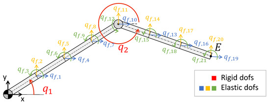
Figure 1. Finite element model of the studied 2-degree-of-freedom (dof) planar manipulator.

Table 2. Finite element model parameters.

Property	Symbol	Value
Length first link	$L_1$	$0.6$ m
Length second link	$L_2$	$0.45$ m
Bending moment of inertia	J	$3.97·{10}^{-8}$${\mathrm{m}}^4$
Circular cross-sectional area	A	$7.06·{10}^{-4}$${\mathrm{m}}^2$
Mass density	$\rho$	2700 $\mathrm{kg}/{\mathrm{m}}^3$
Linear mass density	${\rho }_l$	1.906 $\mathrm{kg}/\mathrm{m}$
Young’s modulus	E	$69·{10}^9$$\mathrm{Pa}$
Mass proportional damping coefficients	$\alpha$	$8.7·{10}^{-1}$ m/s
Stiffness proportional damping coefficients	$\beta$	$4.5·{10}^{-6}$ m·s

To test the correctness of the method in approximating the eigenpairs under motion condition, the system is forced to follow a given trajectory. In particular, the end-effector (point E in Figure 1) moves along a horizontal linear path of 0.3 m in 0.5 s. The corresponding trajectory in the joint coordinates is shown in Figure 2.

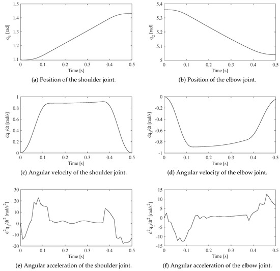
Figure 2. Joint trajectory.

To apply the method under investigation, the system dynamic model has been linearized about a dynamic equilibrium configuration: ${\mathit{P}}_0=({\mathbf{q}}_0=\mathbf{q}(T/2),{\dot{\mathbf{q}}}_0=\dot{\mathbf{q}}(T/2),{\ddot{\mathbf{q}}}_0=\ddot{\mathbf{q}}(T/2),{\mathbf{u}}_0=\mathbf{u}(T/2))$, where T is the time period of the trajectory, the numerical values of the dynamic equilibrium configuration are stated in Appendix A.2. Then, the linearized system has been parameterized on the positions and velocities of the rigid motion coordinates, i.e., $\mathbf{x}={\left\{\begin{array}{cccc}{q}_1& q_2& {\dot{q}}_1& {\dot{q}}_2\end{array}\right\}}^{\mathrm{T}}$. Starting from the solution of the eigenvalue problem computed at the expansion point $\mathbf{x}={\mathbf{x}}_0={\left\{\begin{array}{cccc}{q}_1(T/2)& q_2(T/2)& {\dot{q}}_1(T/2)& {\dot{q}}_2(T/2)\end{array}\right\}}^{\mathrm{T}}$, the eigenpair derivatives up to the fourth Taylor series expansion have been computed by means of Equation (28). Finally, fourth-grade polynomials, representing the eigenvalues and eigenvectors as function of the angular positions and velocities of the shoulder and the elbow joints, have been obtained.

The approximated eigenpairs have been compared with the exact ones, which are computed linearizing the model at each sample time ($\Delta t=0.01$ s) and solving the corresponding eigenvalue problem. In particular, for comparison, the following indices have been employed,

• relative percentage error on the undamped natural frequency, ${ϵ}_f$:

  $${ϵ}_f={\displaystyle \frac{|f-\tilde{f}|}{f}}·100$$

  (30)
  Let $\lambda ={\lambda }_r+i{\lambda }_i$ be a system eigenvalue, it holds:

  $$\omega =\sqrt{{\lambda }_r^2+{\lambda }_i^2};f={\displaystyle \frac{\omega }{2\pi }}$$

  (31)
• relative percentage error on the damping factor, ${ϵ}_{\xi }$:

  $${ϵ}_{\xi }={\displaystyle \frac{|\xi -\tilde{\xi }|}{\xi }}·100;\xi =-{\displaystyle \frac{{\lambda }_r}{\omega }}$$

  (32)
• modal assurance criterion (MAC):

  $$MAC={\displaystyle \frac{{\left|{\mathit{\varphi }}^{*}\tilde{\mathit{\varphi }}\right|}^2}{\left({\tilde{\mathit{\varphi }}}^{*}\tilde{\mathit{\varphi }}\right)\left({\mathit{\varphi }}^{*}\mathit{\varphi }\right)}}$$

  (33)

In Equations (30), (32) and (33), the over-set tilde denotes the approximated quantities. The target value for the comparison of the adopted indices is 1 for the $MAC$ and 0 for ${ϵ}_f$ and ${ϵ}_{\xi }$.

The comparison indices for the first three elastic pairs of complex conjugate eigenvalues and eigenvectors are shown in Figure 3, Figure 4 and Figure 5. The same figures also show the trend of the undamped eigenfrequencies and of the damping ratio along the trajectory, to provide an evidence of the variability of the modal parameters due to system configuration change. All the three figures show a good agreement between the exact and the approximated modal parameters along almost the entire trajectory. The biggest discrepancies (but still bounded) occur on the tails of the trajectory (at the beginning and the end), where the expansion parameters differ significantly from the values they assumed at the expansion point. Overall, the results appear very satisfying for all the three comparison metrics adopted.

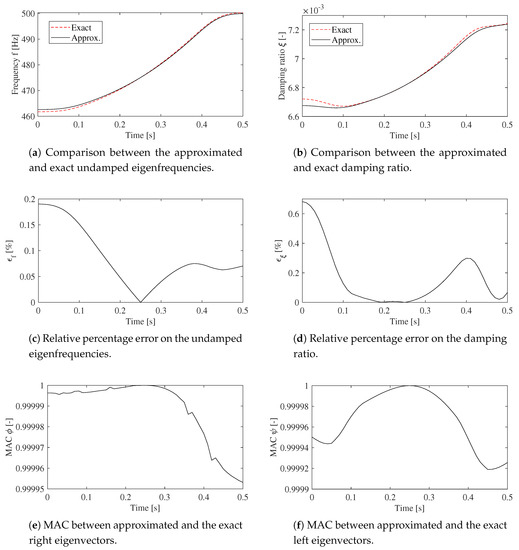
Figure 3. Second vibration mode along the planned trajectory.

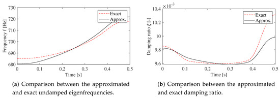
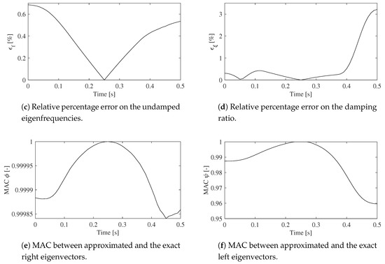
Figure 4. Third vibration mode along the planned trajectory.

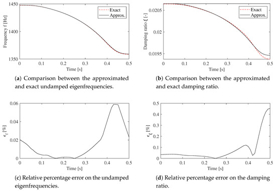
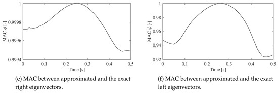
Figure 5. Fourth vibration mode along the planned trajectory.

Finally, note that, although the system has been parameterized around a dynamic equilibrium configuration, the computational time has been drastically reduced. Indeed, the solution of the eigenvalue problem in the 51 operating points in which the trajectory has been discretized requires approximately 0.135 s with a Matlab implementation on a machine with one processor of the type Intel Core i5-6200U CPU at 2.4 GHz with 8 gigabyte of RAM. Conversely, the computation of the approximations of the analyzed eigenpairs in the same points takes on average 0.008 s, leading to a reduction of the computation time of 94%.

5. Conclusions

This paper has outlined the entire procedure to get an analytical polynomial expression of the eigenpairs of a flexible-link multibody system (FMBS) as function of its configuration, in terms of rigid-body motion coordinates and velocities. The method is suitable for FMBSs characterized by small deformations, whose dynamic model is analytically known and formulated by means of a minimum set of ordinary differential equations. Starting from a dynamic model linearized about a static or dynamic equilibrium configuration, the eigenvalue problem in such a configuration is computed. By iteratively expanding the eigenvalue problem in a Taylor series with respect to the rigid motion coordinates, their velocities, and, possibly, the parameters which the system model can depend on (e.g., payload mass), the eigenpair derivatives at the expansion points are inferred. These terms represent the coefficients of the polynomial functions describing the approximated eigenpairs.

The correctness of the method in approximating the system eigenpairs under motion condition (while reducing the computational time), has been numerically proved with satisfactory results by employing a two-dof flexible planar manipulator forced to follow a given trajectory. An experimental validation of the method both in static and dynamic conditions will be addressed in future works by means of an impact analysis and an operational modal analysis, respectively.

The availability of a polynomial function for the eigenpairs explicitly depending on the system configuration can result very helpful for model-based techniques that need an accurate knowledge of the system modal characteristics, such as motion planning and control strategies towards to zero residual vibration.

The method allows to reach a desired accuracy in the eigenpair approximation by selecting the proper expansion order of the Taylor series. However, the selection of a high expansion order could compromise the computational benefits, as the number of addends of the polynomial functions that approximate the eigenpairs rapidly increases with the expansion order. Further research will focus on the development of an index that allows a priori estimation of the proper order of the truncated Taylor series to reach a desired accuracy on the approximated eigensolutions while preserving the computational efficiency.

Appendix A.1. Nonlinear Dynamic Model

The nonlinear dynamic model of the studied planar flexible-link mechanism, obtained through the equivalent rigid-link mechanism formulation, takes the form of Equation (1). The coordinate vector contains the following 21 elastic coordinates and 2 rigid coordinates, whose physical meaning can be inferred from Figure 1.

$$\mathbf{q}=\left\{\begin{array}{c}{q}_{f,1}\\ q_{f,2}\\ q_{f,13}\\ q_{f,4}\\ q_{f,5}\\ q_{f,6}\\ q_{f,7}\\ q_{f,8}\\ q_{f,9}\\ q_{f,10}\\ q_{f,11}\\ q_{f,12}\\ q_{f,13}\\ q_{f,14}\\ q_{f,15}\\ q_{f,16}\\ q_{f,17}\\ q_{f,18}\\ q_{f,19}\\ q_{f,20}\\ q_{f,21}\\ q_1\\ q_2\end{array}\right\}$$

(A1)

The force vector (see Equation (A2)) includes the effects of the gravity forces and the two torques, $u_1$ and $u_2$, acting on the shoulder and elbow joints, respectively.

The stiffness, mass, and damping matrices for this system are shown in Equations (A3)–(A5), respectively. The symbols used in these equations are those defined in Table 2.

$${\mathbf{f}}^{\mathrm{T}}=\left\{\begin{array}{ccccccccccccccccccccccc}0& -{\displaystyle \frac{{\rho }_l{L}_{1}g}{4}}& 0& 0& -{\displaystyle \frac{{\rho }_l{L}_{1}g}{4}}& 0& 0& -{\displaystyle \frac{{\rho }_l{L}_{1}g}{4}}& 0& 0& -{\displaystyle \frac{{\rho }_l(3L_1+4L_2)g}{24}}& -u_2+{\displaystyle \frac{{\rho }_l{L}_1^{2}gcos(q_1)}{192}}& 0& -{\displaystyle \frac{{\rho }_l{L}_{2}g}{3}}& 0& 0& -{\displaystyle \frac{{\rho }_l{L}_{2}g}{3}}& 0& 0& -{\displaystyle \frac{{\rho }_l{L}_{2}g}{6}}& {\displaystyle \frac{{\rho }_l{L}_2^{2}gcos(q_2)}{108}}& u_1-u_2-{\displaystyle \frac{{\rho }_l{L}_1(L_1+2L_2)gcos(q_1)}{2}}& u_2-{\displaystyle \frac{{\rho }_l{L}_2^{2}gcos(q_2)}{2}}\end{array}\right\}$$

(A2)

$$\begin{array}{ccc}\hfill \mathbf{K}& =& \left[\begin{array}{cc}{\mathbf{K}}_{11}& \mathbf{0}\\ \mathbf{0}& \mathbf{0}\end{array}\right]\hfill \\ \hfill {\mathbf{K}}_{11}& =& \left[\begin{array}{ccccccccccccccccccccc}2k_2& -2k_5& 0& k_3& k_5& -k_6& 0& 0& 0& 0& 0& 0& 0& 0& 0& 0& 0& 0& 0& 0& 0\\ & 2k_1& 0& k_5& k_4& k_7& 0& 0& 0& 0& 0& 0& 0& 0& 0& 0& 0& 0& 0& 0& 0\\ & & 2k_8& k_6& -k_7& k_8& 0& 0& 0& 0& 0& 0& 0& 0& 0& 0& 0& 0& 0& 0& 0\\ & & & 2k_2& -2k_5& 0& k_3& k_5& -k_6& 0& 0& 0& 0& 0& 0& 0& 0& 0& 0& 0& 0\\ & & & & 2k_1& 0& k_5& k_4& k_7& 0& 0& 0& 0& 0& 0& 0& 0& 0& 0& 0& 0\\ & & & & & 2k_8& k_6& -k_7& k_8& 0& 0& 0& 0& 0& 0& 0& 0& 0& 0& 0& 0\\ & & & & & & 2k_2& -2k_5& 0& k_3& k_5& -k_6& 0& 0& 0& 0& 0& 0& 0& 0& 0\\ & & & & & & & 2k_1& 0& k_5& k_4& k_7& 0& 0& 0& 0& 0& 0& 0& 0& 0\\ & & & & & & & & 2k_8& k_6& -k_7& k_8& 0& 0& 0& 0& 0& 0& 0& 0& 0\\ & & & & & & & & & k_2+k_{10}& -k_5-k_{13}& k_6& k_{11}& k_{13}& -k_{14}& 0& 0& 0& 0& 0& 0\\ & & & & & & & & & & k_1+k_9& -k_7& k_{13}& k_{12}& k_{15}& 0& 0& 0& 0& 0& 0\\ & & & & & & & & & & & 4k_8& 0& 0& 0& 0& 0& 0& 0& 0& 0\\ & & & & & & & & & & & & 2k_{10}& -2k_{13}& 0& k_{11}& k_{13}& -k_{14}& 0& 0& 0\\ & & & & & & & & & & & & & 2k_9& 0& k_{13}& k_{12}& k_{15}& 0& 0& 0\\ & & & & & & & & & & & & & & 2k_{16}& k_{14}& -k_{15}& k_{16}& 0& 0& 0\\ & & & & & & & & & & & & & & & 2k_{10}& -2k_{13}& 0& k_{11}& k_{13}& -k_{14}\\ & & & & & & & & & & & & & & & & 2k_9& 0& k_{13}& k_{12}& k_{15}\\ & & & & & & & & & & & & & & & & & 2k_{16}& k_{14}& -k_{15}& k_{16}\\ & & & sym.& & & & & & & & & & & & & & & k_{10}& -k_{13}& k_{14}\\ & & & & & & & & & & & & & & & & & & & k_9& -k_{15}\\ & & & & & & & & & & & & & & & & & & & & 4k_{16}\end{array}\right]\hfill \\ \hfill & \hfill & \begin{array}{cccc}{k}_1={\displaystyle \frac{4AEsin{(q_1)}^2}{L_1}}-{\displaystyle \frac{768EJ(sin{(q_1)}^2-1)}{L_1^3}}\hfill & k_2={\displaystyle \frac{4AEcos{(q_1)}^2}{L_1}}-{\displaystyle \frac{768EJ(cos{(q_1)}^2-1)}{L_1^3}}\hfill & k_3={\displaystyle \frac{4AE(sin{(q_1)}^2-1)}{L_1}}-{\displaystyle \frac{768EJsin{(q_1)}^2}{L_1^3}}\hfill & k_4={\displaystyle \frac{4AE(cos{(q_1)}^2-1)}{L_1}}-{\displaystyle \frac{768EJcos{(q_1)}^2}{L_1^3}}\hfill \\ k_5={\displaystyle \frac{2Esin(2q_1)(-A{L}_1^2+192J)}{L_1^3}}\hfill & k_6={\displaystyle \frac{96EJsin(q_1)}{L_1^2}}\hfill & k_7={\displaystyle \frac{96EJcos(q_1)}{L_1^2}}\hfill & k_8={\displaystyle \frac{8EJ}{L_1}}\hfill \\ k_9={\displaystyle \frac{3AEsin{(q_2)}^2}{L_2}}-{\displaystyle \frac{324EJ(sin{(q_2)}^2-1)}{L_2^3}}\hfill & k_{10}={\displaystyle \frac{3AEcos{(q_2)}^2}{L_2}}-{\displaystyle \frac{324EJ(cos{(q_2)}^2-1)}{L_2^3}}\hfill & k_{11}={\displaystyle \frac{3AE(sin{(q_2)}^2-1)}{L_2}}-{\displaystyle \frac{324EJsin{(q_2)}^2}{L_2^3}}\hfill & k_{12}={\displaystyle \frac{3AE(cos{(q_2)}^2-1)}{L_2}}-{\displaystyle \frac{324EJcos{(q_2)}^2}{L_2^3}}\hfill \\ k_{13}={\displaystyle \frac{3Esin(2q_2)(-A{L}_2^2+108J)}{2L_2^3}}\hfill & k_{14}={\displaystyle \frac{54EJsin(q_2)}{L_2^2}}\hfill & k_{15}={\displaystyle \frac{54EJcos(q_2)}{L_2^2}}\hfill & k_{16}={\displaystyle \frac{6EJ}{L_2}}\hfill \end{array}\hfill \end{array}$$

(A3)

$$\begin{array}{ccc}\hfill \mathbf{M}& =& \left[\begin{array}{cc}{\mathbf{M}}_{11}& {\mathbf{M}}_{21}^{\mathrm{T}}\\ {\mathbf{M}}_{21}& {\mathbf{M}}_{22}\end{array}\right]\hfill \\ \hfill {\mathbf{M}}_{11}& =& \left[\begin{array}{ccccccccccccccccccccc}{m}_1& -m_5& 0& -m_3& {\displaystyle \frac{m_5}{2}}& {\displaystyle \frac{13m_6}{840}}& 0& 0& 0& 0& 0& 0& 0& 0& 0& 0& 0& 0& 0& 0& 0\\ & m_2& 0& {\displaystyle \frac{m_5}{2}}& -m_4& -{\displaystyle \frac{13m_7}{840}}& 0& 0& 0& 0& 0& 0& 0& 0& 0& 0& 0& 0& 0& 0& 0\\ & & {\displaystyle \frac{2m_8}{7}}& -{\displaystyle \frac{13m_6}{840}}& {\displaystyle \frac{13m_7}{840}}& -{\displaystyle \frac{3m_8}{28}}& 0& 0& 0& 0& 0& 0& 0& 0& 0& 0& 0& 0& 0& 0& 0\\ & & & m_1& -m_5& 0& -m_3& {\displaystyle \frac{m_5}{2}}& {\displaystyle \frac{13m_6}{840}}& 0& 0& 0& 0& 0& 0& 0& 0& 0& 0& 0& 0\\ & & & & m_2& 0& {\displaystyle \frac{m_5}{2}}& -m_4& -{\displaystyle \frac{13m_7}{840}}& 0& 0& 0& 0& 0& 0& 0& 0& 0& 0& 0& 0\\ & & & & & {\displaystyle \frac{2m_8}{7}}& -{\displaystyle \frac{13m_6}{84}}0& {\displaystyle \frac{13m_7}{840}}& -{\displaystyle \frac{3m_8}{28}}& 0& 0& 0& 0& 0& 0& 0& 0& 0& 0& 0& 0\\ & & & & & & m_1& -m_5& 0& -m_3& {\displaystyle \frac{m_5}{2}}& {\displaystyle \frac{13m_6}{840}}& 0& 0& 0& 0& 0& 0& 0& 0& 0\\ & & & & & & & m_2& 0& {\displaystyle \frac{m_5}{2}}& -m_4& -{\displaystyle \frac{13m_7}{840}}& 0& 0& 0& 0& 0& 0& 0& 0& 0\\ & & & & & & & & {\displaystyle \frac{2m_8}{7}}& -{\displaystyle \frac{13m_6}{840}}& {\displaystyle \frac{13m_7}{840}}& -{\displaystyle \frac{3m_8}{28}}& 0& 0& 0& 0& 0& 0& 0& 0& 0\\ & & & & & & & & & {\displaystyle \frac{m_1+m_9}{2}}& -{\displaystyle \frac{m_5}{2}}-{\displaystyle \frac{m_{13}}{2}}& {\displaystyle \frac{11m_6}{420}}& -m_{11}& {\displaystyle \frac{m_{13}}{2}}& {\displaystyle \frac{13m_{14}}{420}}& 0& 0& 0& 0& 0& 0\\ & & & & & & & & & & {\displaystyle \frac{m_2+m_{10}}{2}}& -{\displaystyle \frac{11m_7}{420}}& {\displaystyle \frac{m_{13}}{2}}& -m_{12}& -{\displaystyle \frac{13m_{15}}{420}}& 0& 0& 0& 0& 0& 0\\ & & & & & & & & & & & {\displaystyle \frac{m_8}{7}}& 0& 0& 0& 0& 0& 0& 0& 0& 0\\ & & & & & & & & & & & & m_9& -m_{13}& 0& -m_{11}& {\displaystyle \frac{m_{13}}{2}}& {\displaystyle \frac{13m_{14}}{420}}& 0& 0& 0\\ & & & & & & & & & & & & & m_{10}& 0& {\displaystyle \frac{m_{13}}{2}}& -m_{12}& -{\displaystyle \frac{13m_{15}}{420}}& 0& 0& 0\\ & & & & & & & & & & & & & & {\displaystyle \frac{2m_{16}}{945}}& -{\displaystyle \frac{13m_{14}}{420}}& {\displaystyle \frac{13m_{15}}{420}}& -{\displaystyle \frac{m_{16}}{1260}}& 0& 0& 0\\ & & & & & & & & & & & & & & & m_9& -m_{13}& 0& -m_{11}& {\displaystyle \frac{m_{13}}{2}}& {\displaystyle \frac{13m_{14}}{420}}\\ & & & & & & & & & & & & & & & & m_{10}& 0& {\displaystyle \frac{m_{13}}{2}}& -m_{12}& -{\displaystyle \frac{13m_{15}}{420}}\\ & & & & & & & & & & & & & & & & & {\displaystyle \frac{2m_{16}}{945}}& -{\displaystyle \frac{13m_{14}}{420}}& {\displaystyle \frac{13m_{15}}{420}}& -{\displaystyle \frac{m_{16}}{1260}}\\ & & & sym.& & & & & & & & & & & & & & & {\displaystyle \frac{m_9}{2}}& -{\displaystyle \frac{m_{13}}{2}}& {\displaystyle \frac{11m_{14}}{210}}\\ & & & & & & & & & & & & & & & & & & & {\displaystyle \frac{m_{10}}{2}}& -{\displaystyle \frac{11m_{15}}{210}}\\ & & & & & & & & & & & & & & & & & & & & {\displaystyle \frac{m_{16}}{945}}\end{array}\right]\hfill \\ \hfill {\mathbf{M}}_{21}& =& \left[\begin{array}{ccccccccccccccccccccc}-{\displaystyle \frac{m_6}{2}}& {\displaystyle \frac{m_7}{2}}& m_8& -m_6& m_7& m_8& -{\displaystyle \frac{3m_6}{2}}& {\displaystyle \frac{3m_7}{2}}& m_8& -{\displaystyle \frac{37m_6+20m_{18}}{40}}& {\displaystyle \frac{37m_7+20m_{19}}{40}}& -{\displaystyle \frac{9m_8}{2}}& -m_{18}& m_{19}& 0& -m_{18}& m_{19}& 0& -{\displaystyle \frac{m_{18}}{2}}& {\displaystyle \frac{m_{19}}{2}}& -{\displaystyle \frac{m_{17}}{54}}\\ 0& 0& 0& 0& 0& 0& 0& 0& 0& -{\displaystyle \frac{3m_{14}}{20}}& {\displaystyle \frac{3m_{15}}{20}}& 0& -m_{14}& m_{15}& {\displaystyle \frac{m_{16}}{135}}& -2m_{14}& 2m15& {\displaystyle \frac{m_{16}}{135}}& -{\displaystyle \frac{27m_{14}}{20}}& {\displaystyle \frac{27m_{15}}{20}}& -{\displaystyle \frac{13m_{16}}{540}}\end{array}\right]\hfill \\ \hfill {\mathbf{M}}_{22}& =& \left[\begin{array}{cc}{m}_{20}& m_{17}\\ m_{17}& m_{16}\end{array}\right]\hfill \\ \hfill & \hfill & \begin{array}{cccccccc}{m}_1={\rho }_l{\displaystyle \frac{L_1(4sin{(q_1)}^2+35)}{210}};\hfill & m_2={\rho }_l{\displaystyle \frac{L_1(4cos{(q_1)}^2+35)}{210}};\hfill & m_3={\rho }_l{\displaystyle \frac{L_1(8sin{(q_1)}^2-35)}{840}};\hfill & m_4={\rho }_l{\displaystyle \frac{L_1(8cos{(q_1)}^2-35)}{840}};\hfill & m_5={\rho }_l{\displaystyle \frac{L_{1}sin(2q_1)}{105}};\hfill & m_6={\rho }_l{\displaystyle \frac{L_1^{2}sin(q_1)}{8}};\hfill & m_7={\rho }_l{\displaystyle \frac{L_1^{2}cos(q_1)}{8}};\hfill & m_8={\rho }_l{\displaystyle \frac{L_1^3}{960}};\hfill \\ m_9={\rho }_l{\displaystyle \frac{2L_2(4sin{(q_2)}^2+35)}{315}};\hfill & m_{10}={\rho }_l{\displaystyle \frac{2L_2(4cos{(q_2)}^2+35)}{315}};\hfill & m_{11}={\rho }_l{\displaystyle \frac{L_2(8sin{(q_2)}^2-35)}{630}};\hfill & m_{12}={\rho }_l{\displaystyle \frac{L_2(8cos{(q_2)}^2-35)}{630}};\hfill & m_{13}={\rho }_l{\displaystyle \frac{4L_{2}sin(2q_2)}{315}};\hfill & m_{14}={\rho }_l{\displaystyle \frac{L_2^{2}sin(q_2)}{9}};\hfill & m_{15}={\rho }_l{\displaystyle \frac{L_2^{2}cos(q_2)}{9}};\hfill & m_{16}={\rho }_l{\displaystyle \frac{2L_2^3}{3}};\hfill \\ m_{17}={\rho }_l{\displaystyle \frac{L_1{L}_2^{2}cos(q_1-q_2)}{2}};\hfill & m_{18}={\rho }_l{\displaystyle \frac{L_1{L}_{2}sin(q_1)}{3}};\hfill & m_{19}={\rho }_l{\displaystyle \frac{L_1{L}_{2}cos(q_1)}{3}};\hfill & m_{20}={\rho }_l{\displaystyle \frac{L_1^2(L_1+3L_2)}{3}}\hfill \end{array}\hfill \end{array}$$

(A4)

$$\begin{array}{ccc}\hfill \mathbf{C}& =& \left[\begin{array}{cc}{\mathbf{C}}_{11}+\alpha {\mathbf{M}}_{11}+\beta {\mathbf{K}}_{11}& {\mathbf{C}}_{12}\\ {\mathbf{C}}_{21}+\alpha {\mathbf{M}}_{21}& {\mathbf{C}}_{22}\end{array}\right]\hfill \\ \hfill {\mathbf{C}}_{11}& =& \left[\begin{array}{ccccccccccccccccccccc}2c_1& c_2& 0& -c_1& -{\displaystyle \frac{c_2}{2}}& {\displaystyle \frac{c_5}{30}}& 0& 0& 0& 0& 0& 0& 0& 0& 0& 0& 0& 0& 0& 0& 0\\ -c_3& -2c_1& 0& {\displaystyle \frac{c_3}{2}}& c_1& {\displaystyle \frac{c_4}{30}}& 0& 0& 0& 0& 0& 0& 0& 0& 0& 0& 0& 0& 0& 0& 0\\ 0& 0& 0& {\displaystyle \frac{c_5}{420}}& {\displaystyle \frac{c_4}{420}}& 0& 0& 0& 0& 0& 0& 0& 0& 0& 0& 0& 0& 0& 0& 0& 0\\ -c_1& -{\displaystyle \frac{c_2}{2}}& -{\displaystyle \frac{c_5}{30}}& 2c_1& c_2& 0& -c_1& -{\displaystyle \frac{c_2}{2}}& {\displaystyle \frac{c_5}{30}}& 0& 0& 0& 0& 0& 0& 0& 0& 0& 0& 0& 0\\ {\displaystyle \frac{c_3}{2}}& c_1& -{\displaystyle \frac{c_4}{30}}& -c_3& -2c_1& 0& {\displaystyle \frac{c_3}{2}}& c_1& {\displaystyle \frac{c_4}{30}}& 0& 0& 0& 0& 0& 0& 0& 0& 0& 0& 0& 0\\ -{\displaystyle \frac{c_5}{420}}& -{\displaystyle \frac{c_4}{420}}& 0& 0& 0& 0& {\displaystyle \frac{c_5}{420}}& {\displaystyle \frac{c_4}{420}}& 0& 0& 0& 0& 0& 0& 0& 0& 0& 0& 0& 0& 0\\ 0& 0& 0& -c_1& -{\displaystyle \frac{c_2}{2}}& -{\displaystyle \frac{c_5}{30}}& 2c_1& c_2& 0& -c_1& -{\displaystyle \frac{c_2}{2}}& {\displaystyle \frac{c_5}{30}}& 0& 0& 0& 0& 0& 0& 0& 0& 0\\ 0& 0& 0& {\displaystyle \frac{c_3}{2}}& c_1& -{\displaystyle \frac{c_4}{30}}& -c_3& -2c_1& 0& {\displaystyle \frac{c_3}{2}}& c_1& {\displaystyle \frac{c_4}{30}}& 0& 0& 0& 0& 0& 0& 0& 0& 0\\ 0& 0& 0& -{\displaystyle \frac{c_5}{420}}& -{\displaystyle \frac{c_4}{420}}& 0& 0& 0& 0& {\displaystyle \frac{c_5}{420}}& {\displaystyle \frac{c_4}{420}}& 0& 0& 0& 0& 0& 0& 0& 0& 0& 0\\ 0& 0& 0& 0& 0& 0& -c_1& -{\displaystyle \frac{c_2}{2}}& -{\displaystyle \frac{c_5}{30}}& c_1+c_6& -{\displaystyle \frac{c_2+c_7}{2}}& {\displaystyle \frac{c_5}{20}}& -c_6& -{\displaystyle \frac{c_7}{2}}& {\displaystyle \frac{c_{10}}{15}}& 0& 0& 0& 0& 0& 0\\ 0& 0& 0& 0& 0& 0& {\displaystyle \frac{c_3}{2}}& c_1& -{\displaystyle \frac{c_4}{30}}& {\displaystyle \frac{c_3+c_8}{2}}& -c_1-c_6& {\displaystyle \frac{c_4}{20}}& {\displaystyle \frac{c_8}{2}}& c_6& {\displaystyle \frac{c_9}{15}}& 0& 0& 0& 0& 0& 0\\ 0& 0& 0& 0& 0& 0& -{\displaystyle \frac{c_5}{420}}& -{\displaystyle \frac{c_4}{420}}& 0& {\displaystyle \frac{c_5}{420}}& {\displaystyle \frac{c_4}{420}}& 0& 0& 0& 0& 0& 0& 0& 0& 0& 0\\ 0& 0& 0& 0& 0& 0& 0& 0& 0& -c_6& -{\displaystyle \frac{c_7}{2}}& 0& 2c_6& c_7& 0& -c_6& -{\displaystyle \frac{c_7}{2}}& {\displaystyle \frac{c_{10}}{15}}& 0& 0& 0\\ 0& 0& 0& 0& 0& 0& 0& 0& 0& {\displaystyle \frac{c_8}{2}}& c_6& 0& -c_8& -2c_6& 0& {\displaystyle \frac{c_8}{2}}& c_6& {\displaystyle \frac{c_9}{15}}& 0& 0& 0\\ 0& 0& 0& 0& 0& 0& 0& 0& 0& -{\displaystyle \frac{c_{10}}{210}}& -{\displaystyle \frac{c_9}{210}}& 0& 0& 0& 0& {\displaystyle \frac{c_{10}}{210}}& {\displaystyle \frac{c_9}{210}}& 0& 0& 0& 0\\ 0& 0& 0& 0& 0& 0& 0& 0& 0& 0& 0& 0& -c_6& -{\displaystyle \frac{c_7}{2}}& -{\displaystyle \frac{c_{10}}{15}}& 2c_6& c_7& 0& -c_6& -{\displaystyle \frac{c_7}{2}}& {\displaystyle \frac{c_{10}}{15}}\\ 0& 0& 0& 0& 0& 0& 0& 0& 0& 0& 0& 0& {\displaystyle \frac{c_8}{2}}& c_6& -{\displaystyle \frac{c_9}{15}}& -c_8& -2c_6& 0& {\displaystyle \frac{c_8}{2}}& c_6& {\displaystyle \frac{c_9}{15}}\\ 0& 0& 0& 0& 0& 0& 0& 0& 0& 0& 0& 0& -{\displaystyle \frac{c_{10}}{210}}& -{\displaystyle \frac{c_9}{210}}& 0& 0& 0& 0& {\displaystyle \frac{c_{10}}{210}}& {\displaystyle \frac{c_9}{210}}& 0\\ 0& 0& 0& 0& 0& 0& 0& 0& 0& 0& 0& 0& 0& 0& 0& -c_6& -{\displaystyle \frac{c_7}{2}}& -{\displaystyle \frac{c_{10}}{15}}& c_6& {\displaystyle \frac{c_7}{2}}& {\displaystyle \frac{c_{10}}{10}}\\ 0& 0& 0& 0& 0& 0& 0& 0& 0& 0& 0& 0& 0& 0& 0& {\displaystyle \frac{c_8}{2}}& c_6& -{\displaystyle \frac{c_9}{15}}& -{\displaystyle \frac{c_8}{2}}& -c_6& {\displaystyle \frac{c_9}{10}}\\ 0& 0& 0& 0& 0& 0& 0& 0& 0& 0& 0& 0& 0& 0& 0& -{\displaystyle \frac{c_{10}}{210}}& -{\displaystyle \frac{c_9}{210}}& 0& {\displaystyle \frac{c_{10}}{210}}& {\displaystyle \frac{c_9}{210}}& 0\end{array}\right];{\mathbf{C}}_{12}=\left[\begin{array}{cc}-{\displaystyle \frac{c_5}{2}}& 0\\ -{\displaystyle \frac{c_4}{2}}& 0\\ 0& 0\\ -c_5& 0\\ -c_4& 0\\ 0& 0\\ -{\displaystyle \frac{3c_5}{2}}& 0\\ -{\displaystyle \frac{3c_4}{2}}& 0\\ 0& 0\\ -{\displaystyle \frac{11c_5+6c_{12}}{12}}& -{\displaystyle \frac{c_{10}}{6}}\\ -{\displaystyle \frac{11c_4+6c_{11}}{12}}& -{\displaystyle \frac{c_9}{6}}\\ 0& 0\\ -c_{12}& -c_{10}\\ -c_{11}& -c_9\\ 0& 0\\ -c_{12}& -2c_{10}\\ -c_{11}& -2c_9\\ 0& 0\\ -{\displaystyle \frac{c_{12}}{2}}& -{\displaystyle \frac{4c_{10}}{3}}\\ -{\displaystyle \frac{c_{11}}{2}}& -{\displaystyle \frac{4c_9}{3}}\\ {\displaystyle \frac{c_{13}{\dot{q}}_1}{54}}& 0\end{array}\right]\hfill \\ \hfill {\mathbf{C}}_{21}& =& \left[\begin{array}{ccccccccccccccccccccc}0& 0& 0& 0& 0& 0& 0& 0& 0& -{\displaystyle \frac{c_5}{60}}& -{\displaystyle \frac{c_4}{60}}& 0& 0& 0& 0& 0& 0& 0& 0& 0& {\displaystyle \frac{c_{13}{\dot{q}}_2}{27}}\\ \\ 0& 0& 0& 0& 0& 0& 0& 0& 0& {\displaystyle \frac{c_{10}}{30}}& {\displaystyle \frac{c_9}{30}}& 0& 0& 0& 0& 0& 0& 0& -{\displaystyle \frac{c_{10}}{30}}& -{\displaystyle \frac{c_9}{30}}& 0\end{array}\right]\hfill \\ \hfill {\mathbf{C}}_{22}& =& \left[\begin{array}{cc}0& c_{13}{\dot{q}}_2\\ c_{13}{\dot{q}}_1& 0\end{array}\right]\hfill \\ \hfill & \hfill & \begin{array}{ccccc}{c}_1={\rho }_l{\displaystyle \frac{L_{1}sin(2p1)}{105}}{\dot{q}}_1& c_2={\rho }_l{\displaystyle \frac{L_1(16sin{(p1)}^2-7)}{420}}{\dot{q}}_1& c_3={\rho }_l{\displaystyle \frac{L_1(16cos{(p1)}^2-7)}{420}}{\dot{q}}_1& c_4={\rho }_l{\displaystyle \frac{L_1^{2}sin(p1)}{8}}{\dot{q}}_1& c_5={\rho }_l{\displaystyle \frac{L_1^{2}cos(p1)}{8}}{\dot{q}}_1\\ c_6={\rho }_l{\displaystyle \frac{4L_{2}sin(2p2)}{315}}{\dot{q}}_2& c_7={\rho }_l{\displaystyle \frac{L_2(16sin{(p2)}^2-7)}{315}}{\dot{q}}_2& c_8={\rho }_l{\displaystyle \frac{L_2(16cos{(p2)}^2-7)}{315}}{\dot{q}}_2& c_9={\rho }_l{\displaystyle \frac{L_2^{2}sin(p2)}{9}}{\dot{q}}_2& c_{10}={\rho }_l{\displaystyle \frac{L_2^{2}cos(p2)}{9}}{\dot{q}}_2\\ c_{11}={\rho }_l{\displaystyle \frac{L_1{L}_{2}sin(p1)}{3}}{\dot{q}}_1& c_{12}={\rho }_l{\displaystyle \frac{L_1{L}_{2}cos(p1)}{3}}{\dot{q}}_1& c_{13}={\rho }_l{\displaystyle \frac{L_1{L}_2^{2}sin(p1-p2)}{2}}\end{array}\hfill \end{array}$$

(A5)

Appendix A.2. Dynamic Equilibrium Configuration

For numerically validating the method, the system dynamic model has been linearized about the following operating point ${\mathbf{P}}_0=({\mathbf{q}}_0,{\dot{\mathbf{q}}}_0,{\ddot{\mathbf{q}}}_0,{\mathbf{u}}_0)$.

$$\begin{array}{ccc}\hfill {\mathbf{q}}_0=\left\{\begin{array}{cc}\hfill 1.2417·{10}^{-5}& \mathrm{m}\hfill \\ \hfill -0.4033·{10}^{-5}& \mathrm{m}\hfill \\ \hfill -16.6300·{10}^{-5}& \mathrm{rad}\hfill \\ \hfill 4.5427·{10}^{-5}& \mathrm{m}\hfill \\ \hfill -1.4656·{10}^{-5}& \mathrm{m}\hfill \\ \hfill -28.9446·{10}^{-5}& \mathrm{rad}\hfill \\ \hfill 9.3360·{10}^{-5}& \mathrm{m}\hfill \\ \hfill -3.0052·{10}^{-5}& \mathrm{m}\hfill \\ \hfill -37.6365·{10}^{-5}& \mathrm{rad}\hfill \\ \hfill 15.1539·{10}^{-5}& \mathrm{m}\hfill \\ \hfill -4.8723·{10}^{-5}& \mathrm{m}\hfill \\ \hfill -43.4043·{10}^{-5}& \mathrm{rad}\hfill \\ \hfill 14.9137·{10}^{-5}& \mathrm{m}\hfill \\ \hfill -4.9993·{10}^{-5}& \mathrm{m}\hfill \\ \hfill -3.2050·{10}^{-5}& \mathrm{rad}\hfill \\ \hfill 14.3918·{10}^{-5}& \mathrm{m}\hfill \\ \hfill -5.2719·{10}^{-5}& \mathrm{m}\hfill \\ \hfill -4.3918·{10}^{-5}& \mathrm{rad}\hfill \\ \hfill 13.7905·{10}^{-5}& \mathrm{m}\hfill \\ \hfill -5.5850·{10}^{-5}& \mathrm{m}\hfill \\ \hfill -4.5621·{10}^{-5}& \mathrm{rad}\hfill \\ \hfill 1.2607& \mathrm{rad}\hfill \\ \hfill 5.1918& \mathrm{rad}\hfill \end{array}\right\};& {\dot{\mathbf{q}}}_0=\left\{\begin{array}{cc}\hfill -9.3747·{10}^{-6}& \mathrm{m}/\mathrm{s}\hfill \\ \hfill 1.5069·{10}^{-5}& \mathrm{m}/\mathrm{s}\hfill \\ \hfill 5.5555·{10}^{-5}& \mathrm{rad}/\mathrm{s}\hfill \\ \hfill 2.5101·{10}^{-5}& \mathrm{m}/\mathrm{s}\hfill \\ \hfill 3.6332·{10}^{-5}& \mathrm{m}/\mathrm{s}\hfill \\ \hfill -4.6108·{10}^{-4}& \mathrm{rad}/\mathrm{s}\hfill \\ \hfill 1.4781·{10}^{-4}& \mathrm{m}/\mathrm{s}\hfill \\ \hfill 4.3995·{10}^{-5}& \mathrm{m}/\mathrm{s}\hfill \\ \hfill -1.0286·{10}^{-3}& \mathrm{rad}/\mathrm{s}\hfill \\ \hfill 3.3005·{10}^{-4}& \mathrm{m}/\mathrm{s}\hfill \\ \hfill 4.2655·{10}^{-5}& \mathrm{m}/\mathrm{s}\hfill \\ \hfill -1.2084·{10}^{-3}& \mathrm{rad}/\mathrm{s}\hfill \\ \hfill 3.3079·{10}^{-4}& \mathrm{m}/\mathrm{s}\hfill \\ \hfill 4.5467·{10}^{-5}& \mathrm{m}/\mathrm{s}\hfill \\ \hfill 1.4025·{10}^{-5}& \mathrm{rad}/\mathrm{s}\hfill \\ \hfill 3.2937·{10}^{-4}& \mathrm{m}/\mathrm{s}\hfill \\ \hfill 5.0324·{10}^{-5}& \mathrm{m}/\mathrm{s}\hfill \\ \hfill 1.5411·{10}^{-7}& \mathrm{rad}/\mathrm{s}\hfill \\ \hfill 3.2637·{10}^{-4}& \mathrm{m}/\mathrm{s}\hfill \\ \hfill 5.5323·{10}^{-5}& \mathrm{m}/\mathrm{s}\hfill \\ \hfill -3.2010·{10}^{-6}& \mathrm{rad}/\mathrm{s}\hfill \\ \hfill 0.8915& \mathrm{rad}/\mathrm{s}\hfill \\ \hfill -0.8640& \mathrm{rad}/\mathrm{s}\hfill \end{array}\right\};& {\ddot{\mathbf{q}}}_0=\left\{\begin{array}{cc}\hfill 0.1512& \mathrm{m}/{\mathrm{s}}^2\hfill \\ \hfill -0.0482& \mathrm{m}/{\mathrm{s}}^2\hfill \\ \hfill -0.4931& \mathrm{rad}/{\mathrm{s}}^2\hfill \\ \hfill 0.2510& \mathrm{m}/{\mathrm{s}}^2\hfill \\ \hfill -0.0800& \mathrm{m}/{\mathrm{s}}^2\hfill \\ \hfill -0.4289& \mathrm{rad}/{\mathrm{s}}^2\hfill \\ \hfill 0.2923& \mathrm{m}/{\mathrm{s}}^2\hfill \\ \hfill -0.0927& \mathrm{m}/{\mathrm{s}}^2\hfill \\ \hfill -0.1383& \mathrm{rad}/{\mathrm{s}}^2\hfill \\ \hfill 0.2896& \mathrm{m}/{\mathrm{s}}^2\hfill \\ \hfill -0.0923& \mathrm{m}/{\mathrm{s}}^2\hfill \\ \hfill -0.0976& \mathrm{rad}/{\mathrm{s}}^2\hfill \\ \hfill 0.2632& \mathrm{m}/{\mathrm{s}}^2\hfill \\ \hfill -0.1047& \mathrm{m}/{\mathrm{s}}^2\hfill \\ \hfill -0.1846& \mathrm{rad}/{\mathrm{s}}^2\hfill \\ \hfill 0.2207& \mathrm{m}/{\mathrm{s}}^2\hfill \\ \hfill -0.1268& \mathrm{m}/{\mathrm{s}}^2\hfill \\ \hfill -0.3827& \mathrm{rad}/{\mathrm{s}}^2\hfill \\ \hfill 0.1639& \mathrm{m}/{\mathrm{s}}^2\hfill \\ \hfill -0.1564& \mathrm{m}/{\mathrm{s}}^2\hfill \\ \hfill -0.4375& \mathrm{rad}/{\mathrm{s}}^2\hfill \\ \hfill 0.6792& \mathrm{rad}/{\mathrm{s}}^2\hfill \\ \hfill 0.8368& \mathrm{rad}/{\mathrm{s}}^2\hfill \end{array}\right\}\hfill \\ & {\mathbf{u}}_0=\left\{\begin{array}{cc}\hfill 3.4787& Nm\hfill \\ \hfill 0.83091& Nm\hfill \end{array}\right\}& \end{array}$$

(A6)

References

- Boscariol, P.; Richiedei, D. Robust point-to-point trajectory planning for nonlinear underactuated systems: Theory and experimental assessment. Robot. Comput.-Integr. Manuf. 2018, 50, 256–265. [Google Scholar] [CrossRef]
- Damaren, C.J. On the Dynamics and Control of Flexible Multibody Systems with Closed Loops. Int. J. Robot. Res. 2000, 19, 238–253. [Google Scholar] [CrossRef]
- Ouyang, H.; Richiedei, D.; Trevisani, A. Pole assignment for control of flexible link mechanisms. J. Sound Vib. 2013, 332, 2884–2899. [Google Scholar] [CrossRef]
- Cossalter, V.; Doria, A.; Basso, R.; Fabris, D. Experimental analysis of out-of-plane structural vibrations of two-wheeled vehicles. Shock Vib. 2004, 11, 433–443. [Google Scholar] [CrossRef]
- Shabana, A.; Zaher, M.; Recuero, A.; Rathod, C. Study of nonlinear system stability using eigenvalue analysis: Gyroscopic motion. J. Sound Vib. 2011, 330, 6006–6022. [Google Scholar] [CrossRef]
- Brüls, O.; Duysinx, P.; Golinval, J.C. The global modal parameterization for non-linear model-order reduction in flexible multibody dynamics. Int. J. Numer. Methods Eng. 2007, 69, 948–977. [Google Scholar] [CrossRef]
- Ripepi, M.; Masarati, P. Reduced order models using generalized eigenanalysis. Proc. Inst. Mech. Eng. Part K J. Multi-Body Dyn. 2011, 225, 52–65. [Google Scholar] [CrossRef]
- Palomba, I.; Richiedei, D.; Trevisani, A. Energy-Based Optimal Ranking of the Interior Modes for Reduced-Order Models under Periodic Excitation. Shock Vib. 2015, 2015, 348106. [Google Scholar] [CrossRef]
- Palomba, I.; Richiedei, D.; Trevisani, A. A reduction strategy at system level for flexible link multibody systems. Int. J. Mech. Control 2017, 18, 59–68. [Google Scholar]
- Vidoni, R.; Scalera, L.; Gasparetto, A.; Giovagnoni, M. Comparison of model order reduction techniques for flexible multibody dynamics using an equivalent rigid-link system approach. In Proceedings of the 8th ECCOMAS Thematic Conference on Multibody Dynamics, Prague, Czech Republic, 19–22 June 2017; pp. 269–280. [Google Scholar]
- Schulze, A.; Luthe, J.; Zierath, J.; Woernle, C. Investigation of a Model Update Technique for Flexible Multibody Simulation. Comput. Methods Appl. Sci. 2020, 53, 247–254. [Google Scholar] [CrossRef]
- Belotti, R.; Caracciolo, R.; Palomba, I.; Richiedei, D.; Trevisani, A. An Updating Method for Finite Element Models of Flexible-Link Mechanisms Based on an Equivalent Rigid-Link System. Shock Vib. 2018, 2018, 1797506. [Google Scholar] [CrossRef]
- Richiedei, D.; Trevisani, A. Updating of Finite Element Models for Controlled Multibody Flexible Systems Through Modal Analysis. Comput. Methods Appl. Sci. 2020, 53, 264–271. [Google Scholar] [CrossRef]
- Belotti, R.; Richiedei, D.; Trevisani, A. Optimal Design of Vibrating Systems Through Partial Eigenstructure Assignment. J. Mech. Des. Trans. ASME 2016, 138, 071402. [Google Scholar] [CrossRef]
- Wehrle, E.; Concli, F.; Cortese, L.; Vidoni, R. Design optimization of planetary gear trains under dynamic constraints and parameter uncertainty. In Proceedings of the 8th ECCOMAS Thematic Conference on Multibody Dynamics 2017, MBD 2017, Prague, Czech Republic, 19–22 June 2017; pp. 527–538. [Google Scholar]
- Wehrle, E.; Palomba, I.; Vidoni, R. In-operation structural modification of planetary gear sets using design optimization methods. Mech. Mach. Sci. 2019, 66, 395–405. [Google Scholar] [CrossRef]
- Erdman, A.; Sandor, G. Kineto-elastodynamics—A review of the state of the art and trends. Mech. Mach. Theory 1972, 7, 19–33. [Google Scholar] [CrossRef]
- Shabana, A. Flexible Multibody Dynamics: Review of Past and Recent Developments. Multibody Syst. Dyn. 1997, 1, 189–222. [Google Scholar] [CrossRef]
- Dwivedy, S.; Eberhard, P. Dynamic analysis of flexible manipulators, a literature review. Mech. Mach. Theory 2006, 41, 749–777. [Google Scholar] [CrossRef]
- Shabana, A.A. Dynamics of Multibody Systems, 4th ed.; Cambridge University Press: Cambridge, MA, USA, 2013. [Google Scholar] [CrossRef]
- Xie, M. Flexible Multibody System Dynamics: Theory and Applications; CRC Press: New York, NY, USA, 2017; pp. 1–214. [Google Scholar] [CrossRef]
- Palomba, I.; Richiedei, D.; Trevisani, A. Reduced-order observers for nonlinear state estimation in flexible multibody systems. Shock Vib. 2018, 2018, 6538737. [Google Scholar] [CrossRef]
- Choi, D.; Park, J.; Yoo, H. Modal analysis of constrained multibody systems undergoing rotational motion. J. Sound Vib. 2005, 280, 63–76. [Google Scholar] [CrossRef]
- Cossalter, V.; Lot, R.; Maggio, F. The Modal Analysis of a Motorcycle in Straight Running and on a Curve. Meccanica 2004, 39, 1–16. [Google Scholar] [CrossRef]
- Masarati, P. Direct eigenanalysis of constrained system dynamics. Proc. Inst. Mech. Eng. Part K J. Multi-Body Dyn. 2010, 223, 335–342. [Google Scholar] [CrossRef]
- Yang, C.; Cao, D.; Zhao, Z.; Zhang, Z.; Ren, G. A direct eigenanalysis of multibody system in equilibrium. J. Appl. Math. 2012, 2012, 638546. [Google Scholar] [CrossRef]
- González, F.; Masarati, P.; Cuadrado, J.; Naya, M. Assessment of Linearization Approaches for Multibody Dynamics Formulations. J. Comput. Nonlinear Dyn. 2017, 12, 041009. [Google Scholar] [CrossRef]
- Wittmuess, P.; Henke, B.; Tarin, C.; Sawodny, O. Parametric modal analysis of mechanical systems with an application to a ball screw model. In Proceedings of the 2015 IEEE Conference on Control and Applications, CCA2015, Sydney, Australia, 21–23 September 2015; pp. 441–446. [Google Scholar] [CrossRef]
- Wittmuess, P.; Tarin, C.; Sawodny, O. Parametric modal analysis and model order reduction of systems with second order structure and non-vanishing first order term. In Proceedings of the 54th IEEE Conference on Decision and Control, CDC 2015, Osaka, Japan, 15–18 December 2015; pp. 5352–5357. [Google Scholar] [CrossRef]
- Palomba, I.; Vidoni, R.; Wehrle, E. Application of a parametric modal analysis approach to flexible-multibody systems. Mech. Mach. Sci. 2019, 66, 386–394. [Google Scholar] [CrossRef]
- Palomba, I.; Wehrle, E.; Vidoni, R.; Gasparetto, A. Parametric eigenvalue analysis for flexible multibody systems. Mech. Mach. Sci. 2019, 73, 4117–4126. [Google Scholar] [CrossRef]
- Verlinden, O.; Huynh, H.; Kouroussis, G.; Rivière-Lorphèvre, E. Modelling of flexible bodies with minimal coordinates by means of the corotational formulation. Multibody Syst. Dyn. 2018, 42, 495–514. [Google Scholar] [CrossRef]
- Vidoni, R.; Scalera, L.; Gasparetto, A. 3-D erls based dynamic formulation for flexible-link robots: Theoretical and numerical comparison between the finite element method and the component mode synthesis approaches. Int. J. Mech. Control 2018, 19, 39–50. [Google Scholar]
- Vidoni, R.; Gasparetto, A.; Giovagnoni, M. A method for modeling three-dimensional flexible mechanisms based on an equivalent rigid-link system. JVC/J. Vib. Control 2014, 20, 483–500. [Google Scholar] [CrossRef]
- Tisseur, F.; Meerbergen, K. The quadratic eigenvalue problem. SIAM Rev. 2001, 43, 235–286. [Google Scholar] [CrossRef]
- Folland, G. Higher-Order Derivatives and Taylor’s Formula in Several Variables. Available online: https://sites.math.washington.edu/~folland/Math425/taylor2.pdf (accessed on 3 November 2019).
© 2019 by the authors. Licensee MDPI, Basel, Switzerland. This article is an open access article distributed under the terms and conditions of the Creative Commons Attribution (CC BY) license (http://creativecommons.org/licenses/by/4.0/).