Estimating Eddy Dissipation Rate with QAR Flight Big Data

Abstract

Air turbulence (AT) is a typical risk that seriously threatens civil aviation safety. It is typically measured via vertical overload, derived equivalent vertical gust velocity (DEVG), and eddy dissipation rate (EDR), while the last one is the most ideal index. In this study, we combined two traditional methods of EDR estimation and proposed a new procedure to estimated EDR with quick access recorder (QAR) data. It enables us to use the parameters only from QAR data for EDR estimation, which fully reflects the great value of QAR data. We estimated EDR values with QAR data collected by the Civil Aviation Administration of China (CAAC), to present the intensities of air turbulences happened within China from 1 January 2016 to 31 December 2018. This study could also be helpful in evaluating and analyzing causes and early warning of AT risks.

1. Introduction

Air turbulence (AT) is a typical risk that seriously threatens civil aviation safety. It could typically cause sudden airplane shakes, from side to side or up and down, or trembles by itself during the flight [1]. It generally brings about anxieties for airline passengers [2], yet severe turbulences might result in aircrafts thrown up and down sharply and frequently, which makes it difficult for pilots to manipulate the aircraft effectively, and even results in structural damages or casualty accidents in extreme cases. On 11th August, 2015, strong ATs caused injuries to several passengers and crew members. To avoid serious losses, it is rather important to explore the occurrence mechanism, influencing factors, detection, or prediction models for ATs.

AT can be categorized into different types, including convective turbulence, clear air turbulence, low-level thermals, and wake turbulence. It is mainly caused or affected by meteorological factors [3]. Some of them could be observed or anticipated via weather radar onboard, but some cannot be detected intuitively, like clear air turbulence (CAT). A number of studies on AT have been conducted, and several indices have been developed to measure clear AT, like Dutton’s index [4], an objective index by Ellrod and Knapp [5], and a real-time estimation technique of AT severity [6]. For the civil aviation of China, the vertical acceleration (VA), however is generally used for measuring AT [7], empirically identifying them with regarding VA less than 0.3 g (gravity unit) or greater than 1.8 g as an unsafe event due to AT. However, the severity of AT affecting an aircraft could be related to nature of the turbulence, airspeed, mass of the aircraft, and altitude [8]. AT reports simply relying on the VA is, thus, of limited application and aircraft specificity.

In essence, turbulence refers to a fluid motion, which is characterized by nonlinearity, vorticity, diffusivity, and energy dissipation [9]. It could be too complicated to define it precisely [10] but can be broadly regarded as a dissipative flow state with nonlinear fluctuating three-dimensional vorticity [11]. Since the early time of aviation industry, studies on turbulence have been involved in designing geometry parameter of an aircraft via computer simulation techniques [12,13]. Eddy is another useful concept for discussing the mechanism of turbulence [10,14,15], and eddy viscosity is an important property for describing turbulence [16]. In particular, eddy dissipation rate (EDR) could be an ideal measurement for evaluating aircraft vortices due to the ambient atmospheric turbulence [17,18,19]. The World Meteorological Organization (WMO) started to add turbulence monitoring information in the aircraft meteorological data relay (AMDAR) since 2002, where both EDR and derived equivalent vertical gust velocity (DEVG) are reported as measurement indices [8]. Note that VA or DEVG reflects more of turbulent appearances when aircraft going through an atmospheric turbulence zone. Different types of aircrafts, however, may respond distinctively to accelerations due to different configurations, even when they go through areas of the same atmospheric condition. Thus, measuring AT via VA or DEVG could be sensitive to different aircrafts. This characteristic leads to a potentially weak point in studying AT risk with them, particularly in the spatially and temporally perspectives. On the contrary, EDR measures the physical impacts of air flows on AT intensity. It tends to be an ideal measurement for studying AT risks, but experiences difficulty when calculating due to the complicated information required. In particular, EDR is a parameter to determine the amount of energy lost by the viscous forces in the turbulent flow [20]. It is the rate at which the turbulence energy is absorbed by breaking the eddy down into smaller and smaller eddies until it is ultimately converted into heat by viscous forces. It is expressed as the kinetic energy per unit mass per second, with units of velocity squared per second (${\mathrm{m}}^{2/3}{\mathrm{s}}^{-1}$) [21].

EDR represents the transmission rate of the disturbance energy from the larger-scale vortex to the smaller-scale vortex. It characterizes the disturbance state of turbulence in the inertia sub-region and is the key parameter for describing atmospheric turbulence. The larger the EDR is, the stronger the turbulence is [22]. Therefore, EDR is often used to describe the vertical gust spectrum of turbulent air around the aircraft [6]. According to the EDR value, the turbulence intensity is divided into different levels, as shown in

Table 1. Turbulence intensity scaling with respect to eddy dissipation rate (EDR) values.

Turbulence Indicator		$\mathbf{Turbulence}\mathbf{Peak}\mathbf{EDR}\mathbf{(}{\mathit{\epsilon }}^{\frac{\mathbf{1}}{\mathbf{3}}} \mathbf{unit}: {\mathbf{m}}^{\mathbf{2}/\mathbf{3}}{\mathbf{s}}^{\mathbf{-}\mathbf{1}}\mathbf{)}$
		<0.1	0.1–0.2	0.2–0.3	0.3–0.4	0.4–0.5	0.5–0.8	>0.8
Turbulence mean EDR (${\epsilon }^{\frac{\mathbf{1}}{\mathbf{3}}} unit\mathbf{:} m^{\mathbf{2}\mathbf{/}\mathbf{3}}{s}^{\mathbf{-}\mathbf{1}}$)	<0.1	0	1	3	6	10	15	21
	0.1–0.2		2	4	7	11	16	22
	0.2–0.3			5	8	12	17	23
	0.3–0.4				9	13	18	24
	0.4–0.5					14	19	25
	0.5–0.8						20	26
	>0.8							27
Turbulence intensity		steady flight	weak turbulence		moderate turbulence		strong turbulence

.

Quick access recorder (QAR) is an airborne flight data recorder designed to provide quick and easy access to raw flight data [23]. It provides environmental parameters, equipment parameters, and operating parameters of the aircraft during the flight. The data enjoy high time accuracy and strong sequence because of the short sampling interval. Meanwhile, QAR data have the characteristics of being complete, high-precision, real-time, and fine-grained, thus it provides a good data foundation for AT-related research. The Civil Aviation Administration of China (CAAC) has been collecting aircraft QAR data from major domestic airlines since 2016, which laid a good data foundation for this research.

In this paper, we outline a simple method for estimating EDR with QAR data. In Section 2, we introduce the QAR data, three different methods to measure flight turbulence intensity, and present the procedure for estimating EDR with QAR data. The EDR estimating results are given in Section 3 and the conclusion is made in Section 4.

2. Data and Methodology

2.1. QAR Data

Since 1 January 1998, CAAC mandated all aircrafts to install QAR or equivalent equipment. QAR data have been broadly collected and widely used in the field, including flight quality monitoring, flight process visual simulation re-emergence, aircraft maintenance, and accident investigation. It contains thousands of parameters related to a flight process, but we only chose several of them, including dates (Date), time (TIME_R), flight phase (FLIGHT_PHASE), standard air pressure altitude (ALT_STD), corrected sea pressure altitude (ALT_QNH), radio altitude (RALT1), vertical overload (VRTG), longitude (LONP), latitude (LATP), and vertical acceleration (VRTG).

In this study, we used the QAR data provided by China Academy of Civil Aviation Science and Technology ranging from 1 January 2016 to 31 December 2018. QAR data of each flight are recorded in individual data tables. Two types of aircrafts, Airbus and Boeing airplanes, achieved these flights. They are featured with distinctive configurations, even QAR data of different items. Within the raw QAR data, more than 1000 properties related to flight and aircraft are recorded. However, we picked 14 of them for the following calculations. The QAR samples are as presented in

Table 2. Quick access recorder (QAR) samples for EDR estimation.

UTC_MIN_SEC	IAS	VRTG	RALT	PITCH	IVV	ROLL	AOAL	AOAR	MACH	LATP	LONP	WIN_SPD	WIN_DIR
0:20:24	142	1.004	1139	3.9	−921	0	19.3	0	0.285	29.3847	100.034	15	198.3
0:20:25	142	0.984	1133	3.9	−892	0	19.3	0	0.284	29.384	100.0346	16	197.6
0:20:26	142	0.984	1120	3.9	−864	0	19.3	0	0.283	29.3833	100.0346	16	197.6
0:20:27	142	0.977	1112	3.9	−870	−0.35	19	0	0.284	29.3826	100.0346	16	197.6
0:20:28	142	0.949	1102	3.9	−896	−0.35	18.6	0	0.284	29.3819	100.0353	16	197.6
0:20:29	142	0.957	1097	3.9	−917	−0.35	19	0	0.283	29.3812	100.0353	17	199.7
0:20:30	141	0.965	1081	4.2	−919	0	19.3	0	0.282	29.3802	100.0353	17	199.7
0:20:31	140	0.984	1038	4.2	−909	0.35	19.3	0	0.281	29.3795	100.036	17	199.7
0:20:32	140	0.984	1012	4.2	−901	0.35	19.7	0	0.28	29.3788	100.036	17	199.7

, and the attributes are explained in

Table 3. Parameters in the QAR data used for EDR estimation.

Field Name	Interpretation	Unit
IAS	Indicated Airspeed	m/s
VRTG	Vertical acceleration	g
RALT	Radio altitude	feet
PITCH	Control column position	degree
IVV	Instantaneous lifting velocity	feet/min
ROLL	Control wheel position	degree
AOAL	Angle of attack left	degree
AOAR	Angle of attack right	degree
HEIGHT	Height	feet
MACH	Mach Number	-
LATP	Present Positon Latitude	degree
LONP	Present Position Longitude	degree
WIN_SPDR	Wind speed FMC	knot
WIN_DIR	Wind Direction computed	knot

.

2.2. Air Turbulence Measurement

2.2.1. Vertical Overload

In China’s civil aviation industry, vertical overload increment is often used as a basis for diagnosis of air turbulence. Since the overload coefficients of the $x$ direction (longitudinal acceleration of the aircraft) and the $z$ direction (lateral acceleration of the aircraft) are generally small, they are often ignored, and only the overload of the $y$ direction (aircraft vertical acceleration) is considered. The overload increment $\Delta n$ (expressed as a multiple of gravity acceleration g) is expressed as Equation (1):

$$\Delta n=VRTG-1$$

(1)

where $VRTG$ is the vertical acceleration of the flight path point recorded in the QAR data, and is also expressed as a multiple of the gravity acceleration g [24]. When the overload increment $\left|\Delta n\right|>0.2\mathrm{g}$, the point could be regarded as a potential air turbulence point [25].

Table 4. Air turbulence intensity and the corresponding overload increments.

Turbulence Intensity	Overload Increment Range (g)
steady flight	$\left|\Delta n\right|\le 0.2$
weak turbulence	$0.2<\left|\Delta n\right|\le 0.5$
moderate turbulence	$0.5<\left|\Delta n\right|\le 0.8$
strong turbulence	$\left|\Delta n\right|>0.8$

shows how the air turbulence intensity corresponds to an overload increment $\left|\Delta n\right|$.

VA reflects more of the turbulent response of an aircraft passing through the atmospheric turbulence area at different speeds [26]. Different type of aircrafts may have different acceleration responses when they pass through the same atmospheric turbulence zone, so this air turbulence intensity measurement is not suitable for objectively describing the intensity of true atmospheric turbulence [27,28].

2.2.2. DEVG

DEVG focuses on the nature of atmospheric turbulence itself and its impacts on aircraft flying over it. It uses measured aircraft vertical acceleration, aircraft altitude, weight, and other factors to characterize the physical quantities of atmospheric turbulence. It is estimated by vertical acceleration, which takes into account information such as total aircraft weight, flight altitude, airspeed, and air temperature, etc.

In the aircraft meteorological data relay reference manual [28], the World Meteorological Organization (WMO) defined the DEVG estimation method based on the formulations of Truscott [29] and Gill [30], as shown in Equation (2):

$$DEVG=\frac{Am\left|\Delta n\right|}{V}$$

(2)

where $\Delta n$ (unit: $\mathrm{g}$) is the peak value of the aircraft’s vertical acceleration deviating from $1\mathrm{g}$, $m$ (unit: $\mathrm{ton}$) is total weight of the aircraft, $V$ (unit: $\raisebox{1ex}{$\mathrm{m}$}\!\left/ \!\raisebox{-1ex}{$\mathrm{s}$}\right.$) is the air flow rate, and $A$ is a specific parameter mainly dependent on the aircraft type, weakly affected by its weight, altitude, and Mach number. It can be approximated via the following equations, Equations (3) and (4),

$$A=\overline{A}+c_4\left(\overline{A}-c_5\right)\left(\frac{m}{\overline{m}}-1\right),$$

(3)

$$\overline{A}=c_1+\frac{c_2}{c_3+H},$$

(4)

where parameters $c_1$, $c_2$, $c_3$, $c_4$, and $c_5$ refer to specific values could be found in the aircraft meteorological data relay reference manual, referring to “Table 1 Parameters used in the estimation of DEVG” on Page 31 of [28]. Their calculations depend on a specific flight profile, which could be expressed as “take-off at speed $V_1$, accelerate to airspeed $V_c$ by height $h_1$, and maintain the lesser of $V_c$ or Mach $M_c$ to cruise altitude $h_c$. Reverse the procedure in the approaching phase” [28] (Page 28); $\overline{m}$ refers to the reference aircraft weight in tons; $H$ (unit: $\mathrm{thousand}\mathrm{feet}$) is the flight altitude.

DEVG provides another effective measurement of AT, and the relationship between the AT intensity and DEVG range is shown in

Table 5. Air turbulence intensity and the corresponding derived equivalent vertical gust velocity (DEVG).

Turbulence Intensity	$\mathit{D}\mathit{E}\mathit{V}\mathit{G}$
steady flight	$DEVG<2.0\mathrm{m}/\mathrm{s}$
weak turbulence	$2.0\mathrm{m}/\mathrm{s}\le DEVG<4.5\mathrm{m}/\mathrm{s}$
moderate turbulence	$4.5\mathrm{m}/\mathrm{s}\le DEVG<9.0\mathrm{m}/\mathrm{s}$
strong turbulence	$DEVG>9.0\mathrm{m}/\mathrm{s}$

. Although DEVG is roughly related to EDR, it does not represent a true measure of atmospheric turbulence intensity; thus, it is not as widely used in atmospheric turbulence measurement applications as EDR.

2.3. EDR Estimation

Traditionally, EDR can be estimated by the following two alternative methods [31]:

(1) Estimation based on the proportional relationship between the EDR and the RMS (root mean square) vertical acceleration estimated from the aircraft accelerometer data [20]. Since the relationship between them is a function of the response characteristics of the aircraft, it varies with flight altitude, aircraft weight, and airspeed. This method largely relies on detailed and precise airborne data, which are not always easy for its accessibility.

(2) Estimation directly from vertical wind speed [32]. This approach relies less on the information collected on the aircraft. There are two estimation ideas:

• Estimate EDR based on the power spectrum of vertical wind estimates over a discrete frequency range [33].
• Similar to the previous one but using different sampling frequencies and aircraft angle of attack correction [26].

2.3.1. The First Estimation Method

Record the power spectral density of the input vertical gust velocity as ${\varphi }_{wg}\left(\omega \right)$, the vertical acceleration of the aircraft as $\ddot{z}\left(\omega \right)$, input gust as $w_g\left(\omega \right)$, then the power spectral density of the acceleration response can be estimated by analyzing the power spectrum and frequency response linear system of the aircraft’s response to turbulence. As shown in Equation (5):

$${\varphi }_{\ddot{z}}\left(\omega \right)={\left|\frac{\ddot{z}\left(i\omega \right)}{w_g\left(i\omega \right)}\right|}^2{\varphi }_{wg}\left(\omega \right).$$

(5)

The estimation is conducted in the frequency domain, and the above equation is integrated between the frequency segments ${\omega }_1$ and ${\omega }_2$ to obtain the acceleration response energy between the frequency segments ${\widehat{\sigma }}_{\ddot{z}}{}^2$. As shown in Equation (6):

$${\widehat{\sigma }}_{\ddot{z}}{}^2={{\displaystyle \int }}_{{\omega }_1}^{{\omega }_2}{\varphi }_{\ddot{z}}\left(\omega \right)d\omega ={{\displaystyle \int }}_{{\omega }_1}^{{\omega }_2}|\frac{\ddot{z}\left(i\omega \right)}{w_g\left(i\omega \right)}{|}^2{\varphi }_{wg}\left(\omega \right)d\omega .$$

(6)

Introduce band pass filter $H_{bp}\left({\omega }_1,{\omega }_2,\omega \right)$, and Equation (6) can be approximated as Equation (7):

$${\widehat{\sigma }}_{\ddot{z}}{}^2\approx {{\displaystyle \int }}_0^{\infty }|H_{bp}\left({\omega }_1,{\omega }_2,\omega \right){|}^2{\left|\frac{\ddot{z}\left(i\omega \right)}{w_g\left(i\omega \right)}\right|}^2{\varphi }_{wg}\left(\omega \right)d\omega .$$

(7)

For the flight conditions of commercial transport aircraft, the frequency band in which the vertical acceleration response of most rigid-body aircraft occurs corresponds to the inertia sub-range of atmospheric turbulence. Therefore, according to Von K$\acute{a}$rm$\acute{a}$n’s energy spectrum theory [6], Equation (8) can be derived:

$${\widehat{\varphi }}_{wg}\left(\omega \right)=0.7V^{\frac{2}{3}}{\epsilon }^{\frac{2}{3}}{\omega }^{-\frac{5}{3}}$$

(8)

where $V$ is true airspeed of the aircraft through the atmospheric turbulence, and ${\epsilon }^{1/3}$ is the EDR. Substituting Equation (8) into Equation (7), Equation (9) is derived:

$${\widehat{\sigma }}_{\ddot{z}}{}^2=0.7V^{\frac{2}{3}}{\epsilon }^{\frac{2}{3}}{{\displaystyle \int }}_0^{\infty }{\left|H_{bp}\left({\omega }_1,{\omega }_2,\omega \right)\right|}^2{\left|\frac{\ddot{z}\left(i\omega \right)}{w_g\left(i\omega \right)}\right|}^2{\omega }^{-\frac{5}{3}}d\omega .$$

(9)

Seen from Equation (9), the EDR value can be estimated when the aircraft response function and the acceleration response energy are known.

The estimation of the aircraft response function can be obtained by constructing an equation of motion for the aircraft. However, parameters such as the wing and tail reference surface area, which are needed in the solution process, are not provided by QAR data.

Estimating the acceleration response energy requires the following two steps:

• Inverse Fourier transform of bandpass filter function, as show in Equation (10):

  $$h_{bp}\left(t\right)=\frac{1}{2\pi }{{\displaystyle \int }}_{-\infty }^{\infty }{H}_{bp}\left({\omega }_1,{\omega }_2,\omega \right)e^{i\omega t}d\omega .$$

  (10)
• Use the Parseval theorem (assuming local stationary) and then use the convolution theorem to get its approximation, as show in Equation (11):

  $${\widehat{\sigma }}_{\ddot{z}}{}^2\left(t\right)\approx \frac{1}{2T}{{\displaystyle \int }}_{t-T}^{t+T}{\left[{{\displaystyle \int }}_0^{{\tau }_1}{h}_{bp}\left(t_1,t_2,{\tau }_2\right)\ddot{z}\left({\tau }_1-{\tau }_2\right)d{\tau }_2\right]}^{2}d{\tau }_1.$$

  (11)

2.3.2. The Second Estimation Method

As the second method, the EDR estimation formula is shown in Equation (12):

$${\widehat{\epsilon }}^{\frac{1}{3}}={\left(\frac{{\gamma }^2}{k_h-k_l+1}{\displaystyle \sum }_{k=k_l}^{k_h}\frac{{\widehat{S}}_k^w}{S_k^{model}}\right)}^{\frac{1}{2}}$$

(12)

where ${\widehat{\epsilon }}^{1/3}$ is the EDR to be estimated,$\gamma$ is the correction factor, $k_h$ and $k_l$ are the coefficients k corresponding to the high frequency and low frequency, respectively, of the selected frequency interval, and ${\widehat{S}}_k^w$ and $S_k^{model}$ are the measured energy spectrum functions and theoretical energy spectrum functions of turbulent flow, respectively.

The specific estimation steps are as follows:

(1) Estimate the true airspeed (TAS) by indicating airspeed and flight altitude.

(2) Estimate the angle of attack (AOA). Firstly, the average angle of attack is estimated according to the left and right angles of attack of the aircraft. Then, the average angle of attack is corrected according to the correction value estimated by the length of the sensor arm, the pitch rate, and the true airspeed. Finally, the angle of attack based on the body axis is estimated by the angle transformation [34]. In this process, parameters such as the left and right angles of attack of the aircraft and the length of the sensor arm are not provided by the QAR data.

(3) Estimate vertical wind, $w$ based on the body axis, as shown in Equation (13):

$$w=-TAS\left(\cos \theta \sin {\alpha }_b\cos \varnothing -\cos {\alpha }_b\sin \theta \right)-IVV$$

(13)

where $\theta$ is the pitch angle, $\varnothing$ is the roll angle, ${\alpha }_b$ is the aircraft angle of attack estimated in Step (2), and IVV is the inertial vertical speed of the aircraft.

(4) Estimate the vertical wind of the trend wind and windowing function. The vertical wind is transformed based on the estimated matrix.

(5) The vertical wind obtained in Step (4) is subjected to discrete Fourier transform to obtain the turbulent measured energy spectrum, and the theoretical energy spectrum of the turbulent flow is obtained by looking up the “Table 1 Parameters used in the estimation of DEVG” on Page 31 of [28].

In summary, both estimation methods involve parameters that are not provided in the QAR data. It is impossible to estimate the EDR by directly applying the two methods. Therefore, this paper provides a method to approximate the EDR estimation by concerning both methods.

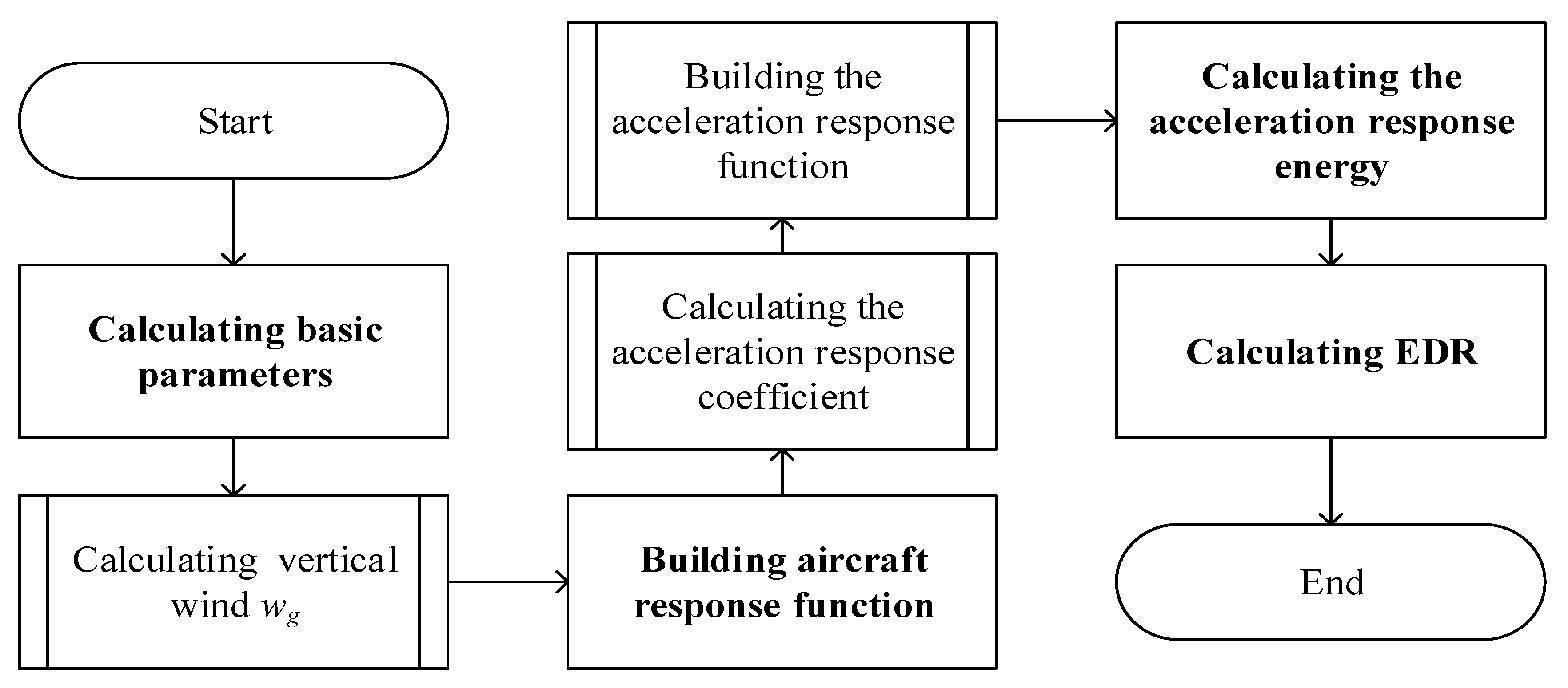
2.3.3. Estimating EDR with QAR Data

As shown in Figure 1, the key to estimate EDR with QAR data is to utilize the QAR records for all the parameter calculations. In this study, we designed a procedure for this calculation, and it is shown in Figure 1 as the following steps:

• Estimate the basic parameter vertical wind $w_g$.
• Build the aircraft response function.
• Estimate the acceleration response energy.
• Estimate EDR.

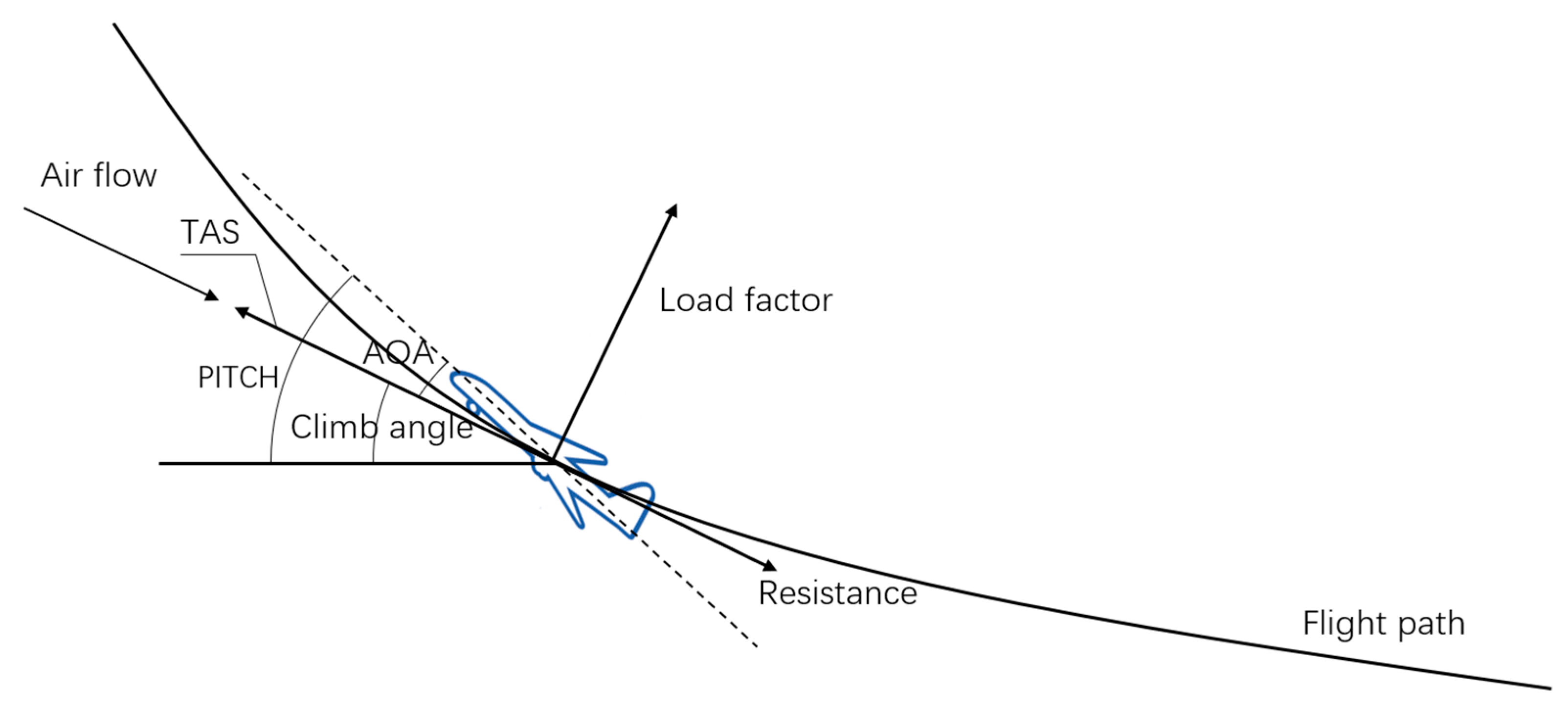
(1) Estimate Basic Parameters

In order to obtain EDR value, the first basic parameter, vertical wind $w_g$, must be estimated. Vertical wind can be estimated from the above parameters, as shown in Equation (14):

$$w_g=-TAS\ast \left(\cos \theta \sin AOA\cos \varphi -\cos AOA\sin \theta \right)-IVV$$

(14)

where $\theta$ is the pitch angle PITCH of the QAR data and $\varnothing$ is the roll angle ROLL of the QAR data. AOA (angle of attack, unit: Radians) refers to the angle between the velocity vector and the aircraft’s string, PITCH (unit: Radians) is the airplane’s pitch angle, IVV (unit: m/s) is the instantaneous hoisting rate, and TAS (unit: m/s) is the true airspeed. Figure 2 exemplifies these attitude angles geometrically.

As shown in Figure 2, the angles of attack recorded by QAR cannot be used directly. They need to be converted into an angle of attack based on the body axis before being used in the calculation of vertical wind. The conversion method can be expressed as follows:

$$AOA=a_0+a_1\left[\frac{(AO{A}_L+AO{A}_R)}{2}+\frac{L\dot{\theta }}{TAS}\right]$$

(15)

where $AO{A}_L$ is the left angle of attack and $AO{A}_R$ is the right angle recorded in QAR. $L$ is the length of the sensor arm, taking half of the fuselage length. $\dot{\theta }$ is the pitch rate. Constants $a_0$ and $a_1$ are estimated using a linear least squares fit of $\theta =a_0+a_1\frac{(AO{A}_L+AO{A}_R)}{2}$ in the preprocessing step, i.e., $a_0=3.19957$, $a_1=0.602594$.

(2) Build the Aircraft Response Function

(1) Estimate the acceleration response coefficient

The Fourier transform is performed on the vertical acceleration VRTG and the vertical wind $w_g$ in the time T (takes 10 s, and recording frequency is 8 Hz), and converts it from the time domain to the frequency domain to obtain $\ddot{z}\left(i\omega \right)$ and $w_g\left(i\omega \right)$ of the nine recorded points in the current estimation window. Taking the value of $\frac{\ddot{z}\left(i\omega \right)}{w_g\left(i\omega \right)}$ constitutes a new sequence of points. Since the equation form of $\frac{\ddot{z}\left(i\omega \right)}{w_g\left(i\omega \right)}$ is unknown and indeterminate, we fit it here via a polynomial curve fitting method. Results show that the cubic polynomial fitting performs the best in terms of both accuracy and efficiency, in comparison to the linear, quadratic, and fourth-order polynomial fitting methods. It can be expressed as Equation (16):

$$\frac{\ddot{z}\left(i\omega \right)}{w_g\left(i\omega \right)}\approx c_0+c_1·\omega +c_2·{\omega }^2+c_3·{\omega }^3.$$

(16)

(2) Build the acceleration response function

The integral of the acceleration response function $I\left(\omega \right)$ can be written as Equation (17):

$$I\left(\omega \right)={{\displaystyle \int }}_{{\omega }_1}^{{\omega }_2}{\left|\frac{\ddot{z}\left(i\omega \right)}{w_g\left(i\omega \right)}\right|}^2{\omega }^{-\frac{5}{3}}d\omega ={{\displaystyle \int }}_{{\omega }_1}^{{\omega }_2}{\left(c_0+c_1·\omega +c_2·{\omega }^2+c_3·{\omega }^3\right)}^2{\omega }^{-\frac{5}{3}}d\omega .$$

(17)

Usually, take ${\omega }_1=0.1\mathrm{HZ},{\omega }_2=0.8\mathrm{HZ}$ to shield high-frequency and low-frequency noise.

(3) Estimate the Acceleration Response Energy

First of all, perform an inverse Fourier transform on the band pass filter function $h_{bp}\left(t\right)$, as shown in Equation (18):

$$h_{bp}\left(t\right)=\frac{1}{2\pi }{{\displaystyle \int }}_{-\infty }^{\infty }{H}_{bp}\left({\omega }_1,{\omega }_2,\omega \right)e^{i\omega t}d\omega .$$

(18)

Then, according to the Parseval theorem (assuming local stationarity), an approximation of the acceleration response energy ${\widehat{\sigma }}_{\ddot{z}}$ can be obtained by convolution, as shown in Equation (19):

$${\widehat{\sigma }}_{\ddot{z}}{}^2\left(t\right)\approx \frac{1}{2T}{{\displaystyle \int }}_{t-T}^{t+T}{\left[{{\displaystyle \int }}_0^{{\tau }_1}{h}_{bp}\left({\tau }_2\right)VRTG\left({\tau }_1-{\tau }_2\right)d{\tau }_2\right]}^{2}d{\tau }_1$$

(19)

where T takes 10 s, and $VRTG\left(t\right)$ is a curve equation obtained by fitting the VRTG value of the recorded points in 2T.

(4) Estimate EDR

Finally, EDR ${\epsilon }^{\frac{1}{3}}$ can be estimated via the Equation (20) [32]:

$${\epsilon }^{\frac{1}{3}}=\sqrt{\frac{{\widehat{\sigma }}_{\ddot{z}}{}^2}{0.7TA{S}^{2/3}I\left(\omega \right)}}.$$

(20)

In this way, EDR could be estimated with the QAR data, where all the parameters are calculated accordingly. In the next section, this procedure will be exemplified with QAR data collected from 1 January 2016 to 31 December 2018.

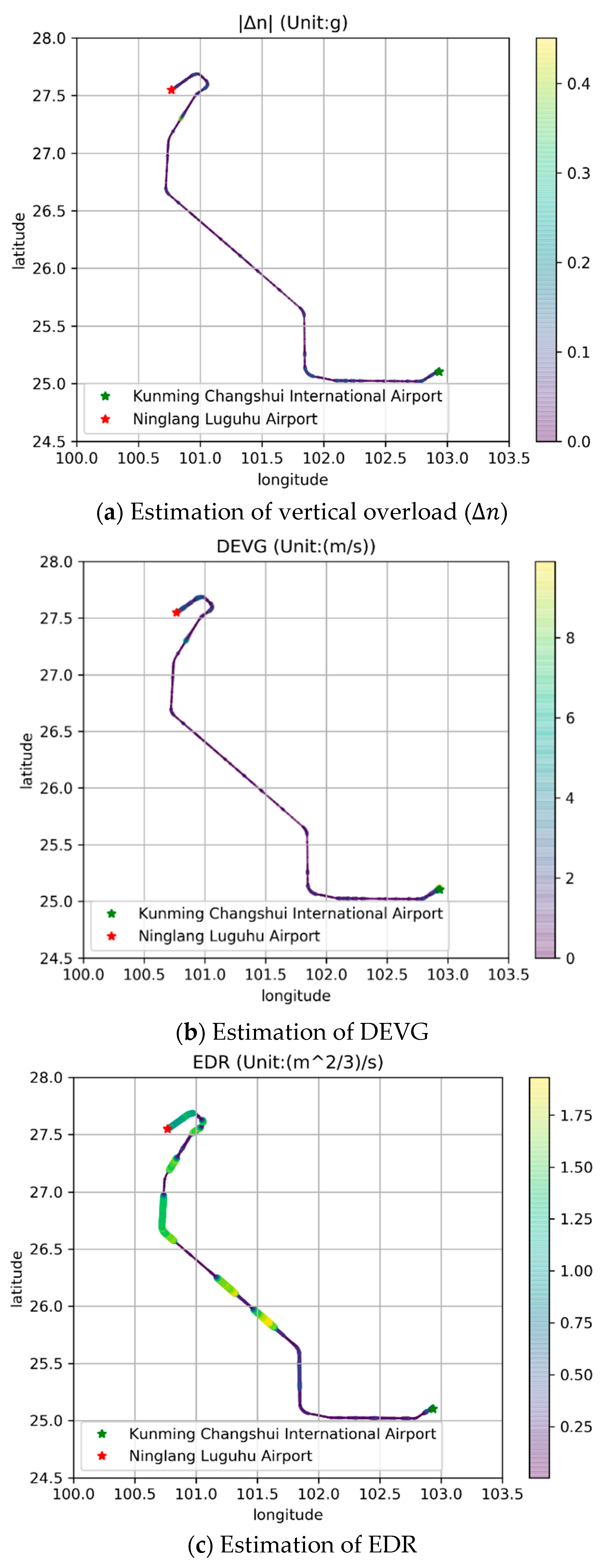
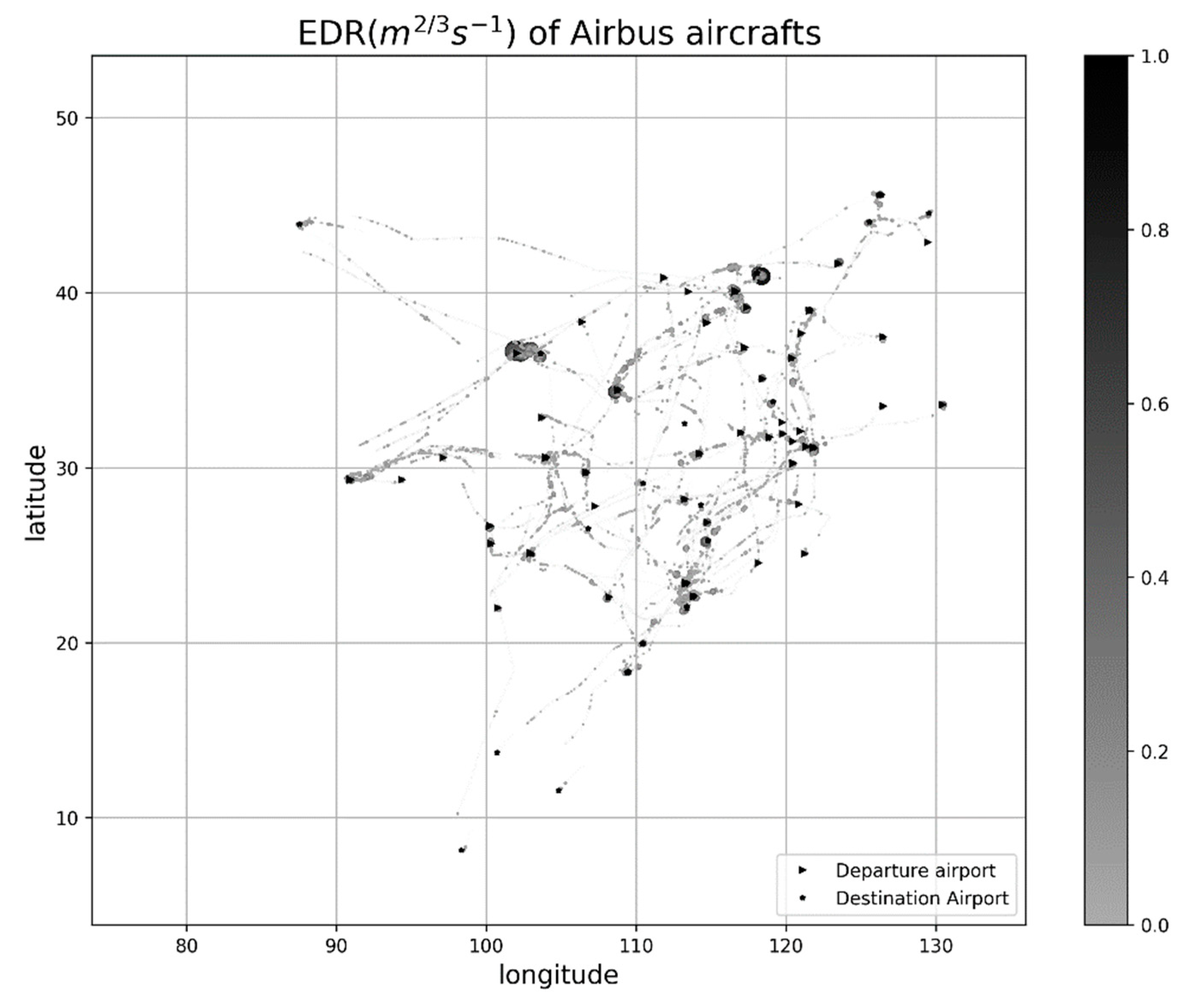
3. Results and Discussion

According to the estimation method described in Section 2, we achieved the vertical overload ($\left|\Delta n\right|$), DEVG and EDR estimations via the Python programming language. First of all, we picked up the QAR data from a flight from Kunming Changshui International Airport to Ninglang Lake Airport on 6 October 2016. Results of the vertical overload ($\left|\Delta n\right|$), DEVG and EDR estimations are as shown in Figure 3a–c. Results show that the estimated $\left|\Delta n\right|$ and DEVG are of similar patterns due to their linearly correlated calculations, while EDR estimations provide a very different perspective on AT risks. The former two indicators report physical bumps happening during the flight, and pointy and discrete AT events can be detected in Figure 3a,b. These results, however, could vary for a different aircraft, even under all the same atmospheric conditions outside. The EDR estimates in Figure 3c present segmented and continuous patterns, which conform with the general perceptions of atmospheric flow. Moreover, the segments of large EDR values match with the bumps presented in Figure 3a,b. All in all, EDR provides a more scientific indicator for evaluating AT risks during a flight than the former two indicators.

EDR provides a measurement of AT risk from outside atmospheric conditions. It is meaningful to visualize the EDR estimates from historical QAR data for exploring AT risks. We thus visualized the EDR estimates with the QAR data collected from 1 January 2016 to 31 December 2018. Note that EDR for the Airbus and Boeing aircrafts are estimated individually due different parameter settings, and we present them in Figure 4 and Figure 5, respectively. The black arrow indicates the approximate location of the departure airport and the black asterisk indicates the approximate location of the destination airport. In this study, we only utilized QAR data of the aircraft flying phrase in the air; the location of departure airports and destination airports is estimated based on the coordinates within the in-air trajectory. For each airline, the darker and bigger the point is, the greater the turbulent strength is anticipated. As seen from Figure 4, the severity of AT for Airbus aircrafts in the northwest region and areas around Beijing is apparently higher than in other areas. In Figure 5, the occurrence of AT for Boeing aircrafts in the southeastern coastal areas is more frequent than in the other areas, and the severity of AT is slightly higher than in other areas. The results provide a good overview on the spatial patterns of AT intensities; particularly, clusters appearing in both Figure 4 and Figure 5 may indicate areas of high AT risks. These hotspots could be related to potential factors for further analysis, for example meteorological, environmental, and terrain factors. This forms a good topic for future studies, particularly fundamental for early-warning studies. Moreover, note that these EDR results are calculated with QAR data collected within three years. The temporal dimension could be incorporated to explore their spatio-temporal patterns, which could provide richer information for specific applications, like flight route planning.

4. Conclusions

On the one hand, AT is a typical risk in the civil aviation industry, and EDR is an ideal physical indicator for measuring its intensity. On the other hand, the collection of QAR data by CAAC provides a super data source for studying such topics, including aviation safety and flight operations quality assurance (FOQA). However, there is no straightforward strategy to calculate EDR with QAR data. Two traditional methods of EDR estimation both involve parameters that could be not provided by the QAR data. In this study, we proposed a practical step-wise procedure to bridge them up, effectively and efficiently. We compared EDR estimations with the corresponding vertical overload and DEVG, and results show that EDR provides a reasonable indicator for evaluating AT risks during a flight. Moreover, with the trillions of pieces of QAR records collected from 1 January 2016 to 31 December 2018, the EDR values for the Airbus and Boeing aircrafts are calculated within an acceptable time cost and visualized spatially. It is interesting for overviewing the spatial patterns, of which hotspots or clusters possibly indicate high risks of AT.

Furthermore, this study also makes a good foundation for a number of further studies in the field of aviation safety and FOQA, such as: (i) Analyzing spatio-temporal patterns of AT risks across China via incorporating the temporal dimension [35]; (ii) exploring potential affecting factors on AT risks, for example meteorological, environmental, and terrain factors via spatial statistics techniques, like geographically weighted regression [36,37]. These future studies will be meaningful for applications in flight route planning, early risk warning, and FOQA.

References

1. Potter, E. Five Myths about Air Turbulence. USA Today. Available online: https://www.usatoday.com/story/travel/flights/2014/07/10/5-myths-about-air-turbulence/12301043/ (accessed on 10 July 2014).
2. Lallanilla, M. Air Turbulence: How Dangerous Is It? Live Science. Available online: https://www.livescience.com/43448-air-turbulence-dangerous-injuries.html (accessed on 18 February 2014).
3. Fultz, A.J.; Ashley, W.S. Fatal weather-related general aviation accidents in the united states. Phys. Geogr. 2016, 37, 291–312. [Google Scholar] [CrossRef]
4. Dutton, J.A.; Panofsky, H.A. Clear air turbulence: A mystery may be unfolding. Science 1970, 167, 937. [Google Scholar] [CrossRef] [PubMed]
5. Ellrod, G.; Knapp, D. An Objective Clear-Air Turbulence Forecasting Technique: Verification and Operational Use. Weather Forecast. 1992, 7, 150–165. [Google Scholar] [CrossRef]
6. Cornman, L.B.; Morse, C.S.; Cunning, G. Real-time estimation of atmospheric turbulence severity from in-situ aircraft measurements. J. Aircr. 1995, 32, 171–177. [Google Scholar] [CrossRef]
7. Wu, Y.; Zhou, L.; Liu, K.; Huang, C.; Shu, Z. AMDAR based statistical analysis on the features of cross-ocean airplane turbulence over china’s surrounding sea areas. J. Meteorol. Sci. 2014, 34, 17–24. [Google Scholar]
8. WMO. Aircraft Meteorological Data Relay (AMDAR) Reference Manual; World Meteorological Organization: Geneva, Switzerland, 2003. [Google Scholar]
9. Markatos, N.C. The mathematical modelling of turbulent flows. Appl. Math. Model. 1986, 10, 190–220. [Google Scholar] [CrossRef]
10. Argyropoulos, C.D.; Markatos, N.C. Recent advances on the numerical modelling of turbulent flows. Appl. Math. Model. 2015, 39, 693–732. [Google Scholar] [CrossRef]
11. Kundu, P.K.; Cohen, I.M.; Dowling, D.R. Fluid Mechanics, 5th ed.; Elsevier: London, UK, 2012. [Google Scholar]
12. Spalding, D.B. A general purpose computer program for multi-dimensional one- and two-phase flow. Math. Comput. Simul. 1981, 23, 267–276. [Google Scholar] [CrossRef]
13. Spalart, P.R. Detached-Eddy Simulation. Annu. Rev. Fluid Mech. 2008, 41, 181–202. [Google Scholar] [CrossRef]
14. Launder, B.E.; Spalding, D.B. Mathematical Models of Turbulence; Academic Press: London, UK, 1972. [Google Scholar]
15. Bradshaw, P. An Introduction to Turbulence and its Measurements; Pergamon: Oxford, UK, 1971. [Google Scholar]
16. Launder, B.E. Heat and mass transport. In Topics in Applied Physics; Bradshaw, P., Ed.; Springer: Berlin, Germany, 1978; Volume 12, pp. 231–287. [Google Scholar]
17. Sarpkaya, T.; Robins, R.E.; Delisi, D.P. Wake-Vortex Eddy-Dissipation Model Predictions Compared with Observations. J. Aircr. 2001, 38, 687–692. [Google Scholar] [CrossRef]
18. Chan, P.W. Generation of an Eddy Dissipation Rate Map at the Hong Kong International Airport Based on Doppler Lidar Data. J. Atmos. Ocean. Technol. 2010, 28, 37–49. [Google Scholar] [CrossRef]
19. Proctor, F.; Hamilton, D. Evaluation of Fast-Time Wake Vortex Prediction Models. In Proceedings of the 47th AIAA Aerospace Sciences Meeting including the New Horizons Forum and Aerospace Exposition, Orlando, FL, USA, 5–8 January 2009; American Institute of Aeronautics and Astronautics: Reston, VA, USA, 2009. [Google Scholar] [CrossRef]
20. MacCready, P.B. Standardization of gustiness values from aircraft. J. Appl. Meteorol. 1964, 3, 439–449. [Google Scholar] [CrossRef]
21. Sharman, R.D.; Pearson, J.M. Prediction of energy dissipation rates for aviation turbulence. Part i: Forecasting nonconvective turbulence. J. Appl. Meteorol. Climatol. 2016, 56, 317–337. [Google Scholar] [CrossRef]
22. Zhou, Y.; Wei, M.; Cheng, Z.; Ning, Y.; Qi, L. The wind and temperature information of AMDAR data applying to the analysis of severe weather nowcasting of airport. In Proceedings of the IEEE Third International Conference on Information Science and Technology, Yangzhou, China, 23–25 March 2013. [Google Scholar]
23. Sun, H.; Jiao, Y.; Han, J.; Wang, C. A novel temporal-spatial analysis system for QAR big data. In Proceedings of the IEEE 17th International Conference on Communication Technology (ICCT), Chengdu, China, 27–30 October 2017; pp. 1238–1241. [Google Scholar]
24. Sun, J.; Lenschow, D.H.; Burns, S.P.; Banta, R.M.; Newsom, R.K.; Coulter, R.; Frasier, S.; Ince, T.; Nappo, C.; Balsley, B.B.; et al. Atmospheric disturbances that generate intermittent turbulence in nocturnal boundary layers. Bound. Layer Meteorol. 2004, 110, 255–279. [Google Scholar] [CrossRef]
25. Sherman, D.J. The Australian Implementation of AMDAR/ACARS and the Use of Derived Equivalent Gust Velocity as a Turbulence Indicator; Department of Defence, Defence Science and Technology Organisation, Aeronautical Research Laboratories Melbourne: Melbourne, Australia, 1985.
26. Haverdings, H.; Chan, P.W. Quick access recorder data analysis software for windshear and turbulence studies. J. Aircr. 2010, 47, 1443–1447. [Google Scholar] [CrossRef]
27. Yuan, J. Application research on aircraft air bump level classification standard. Sci. Technol. 2017, 7, 246. [Google Scholar]
28. SWMO. Aircraft Meteorological Data Relay (AMDAR) Reference Manual; SWMO, Ed.; SWMO: Geneva, Switzerland, 2003. [Google Scholar]
29. Truscott, B. EUMETNET AMDAR AAA AMDAR SOFTWARE Developments—Technical Specification; Doc. Ref.; Met Office: Exeter, UK, 2000.
30. Gill, P.G. Objective verification of world area forecast centre clear air turbulence forecasts. Meteorol. Appl. 2014, 21, 3–11. [Google Scholar] [CrossRef]
31. Kim, S.-H.; Chun, H.-Y.; Chan, P.W. Comparison of turbulence indicators obtained from in situ flight data. J. Appl. Meteorol. Climatol. 2017, 56, 1609–1623. [Google Scholar] [CrossRef]
32. Sharman, R.D.; Cornman, L.B.; Meymaris, G.; Pearson, J.; Farrar, T. Description and derived climatologies of automated in situ eddy-dissipation-rate reports of atmospheric turbulence. J. Appl. Meteorol. Climatol. 2014, 53, 1416–1432. [Google Scholar] [CrossRef]
33. Cornman, L.; Meymaris, G.; Limber, M. An update on the FAA aviation weather research programs in situ turbulence measurement and reporting system. In Proceedings of the 11th Conference on Aviation, Range, and Aerospace Meteorology, Hyannis, MA, USA, 5 October 2004. [Google Scholar]
34. Bach, R.E.; Wingrove, R.C. Applications of state estimation in aircraft flight-data analysis. J. Aircr. 1985, 22, 547–554. [Google Scholar] [CrossRef]
35. Wu, M.; Sun, H.; Wang, C.; Lu, B. Detecting and Analysing Spatial-Temporal Aggregation of Flight Turbulence with the QAR Big Data. In Proceedings of the 2018 26th International Conference on Geoinformatics, Kunming, China, 28–30 June 2018; pp. 1–6. [Google Scholar]
36. Brunsdon, C.; Fotheringham, A.S.; Charlton, M.E. Geographically Weighted Regression: A Method for Exploring Spatial Nonstationarity. Geogr. Anal. 1996, 28, 281–298. [Google Scholar] [CrossRef]
37. Lu, B.; Harris, P.; Charlton, M.; Brunsdon, C. The GWmodel R package: Further topics for exploring spatial heterogeneity using geographically weighted models. Geo-Spat. Inf. Sci. 2014, 17, 85–101. [Google Scholar] [CrossRef]
Figure 1. Procedure of estimating EDR with QAR data.
Applsci 09 05192 g001
Figure 2. Attitude angles of an aircraft.
Applsci 09 05192 g002
Figure 3. Comparisons of vertical overload ( Δ n ), DEVG, and EDR.
Applsci 09 05192 g003
Figure 4. EDR estimation result of Airbus aircrafts.
Applsci 09 05192 g004
Figure 5. EDR estimation result of Boeing aircrafts.
Applsci 09 05192 g005