Primitive Shape Fitting in Point Clouds Using the Bees Algorithm

Abstract

In this study the problem of fitting shape primitives to point cloud scenes was tackled as a parameter optimisation procedure, and solved using the popular bees algorithm. Tested on three sets of clean and differently blurred point cloud models, the bees algorithm obtained performances comparable to those obtained using the state-of-the-art random sample consensus (RANSAC) method, and superior to those obtained by an evolutionary algorithm. Shape fitting times were compatible with real-time application. The main advantage of the bees algorithm over standard methods is that it doesn’t rely on ad hoc assumptions about the nature of the point cloud model like RANSAC approximation tolerance.

1. Introduction

Point clouds (PCs) are widely used in machine vision and robotics to represent 3D scenes and objects sensed through laser scanning devices. Understanding PC models, and extracting concise and meaningful high-level descriptions such as the shape and properties of objects, is necessary for many industrial applications like robotic grasping and pick-and place [1,2]. This ability is naturally acquired by humans and animals, but difficult to reliably automate [3], particularly in real-time applications where time and hardware limitations require very efficient procedures.

This paper is concerned with the identification of the shape of objects in 3D PCs for robot manipulation. In many industrial applications, man-made artefacts can be associated with good approximation to a set of geometrical primitive shapes like spheres, boxes, and cylinders. The problem becomes then to fit these primitive shapes to clusters of points in PC models (the primitive fitting problem). Since PCs are composed of a very large number of points, the efficiency of the identification algorithms is of primary importance. At the same time, for the sake of generality, problem-specific assumptions should be limited.

The primitive fitting problem is well known in the literature, and many of the solutions are based on two popular and very successful algorithms: the Hough transform (HT) [4] and random sample consensus (RANSAC) [5]. Given a 3D scene, the HT looks for parameterisations of primitive shapes that fit the largest number of data points. To increase the efficiency of the HT, the space of the parameterisations may be quantised, and in that case the granularity of the quantisation becomes an important parameter [6]. RANSAC randomly picks from the PC minimal sets of points that are used to parameterise candidate primitive shapes. RANSAC verifies the candidate shapes against the remaining points in the scene, and picks the instance that fits the largest number of points. An approximation tolerance is usually set to decide whether a point is an inlier or outlier to a given shape. The main limitations of the HT and RANSAC are their computational complexity, and the sensitivity of the results to the algorithm parameterisation (the quantisation of parameters in the HT, the approximation tolerance in RANSAC).

The approach proposed in this paper is to tackle primitive fitting as a parameter optimisation problem. Similarly to the HT approach, the goal of the procedure is to manipulate the parameters of a given type of primitive to maximise its fit to the point data. The fit is measured by a primitive-specific fitness function which is used to guide the optimisation process. The bees algorithm (BA) [7] will be used as the parameter optimisation routine, and the results compared with those achieved using an evolutionary algorithm (EA) [8] and RANSAC.

The main advantage of metaheuristics like swarm (bees algorithm) and evolutionary algorithms over standard primitive fitting techniques is the generality of the approach, which does not require prior scene knowledge (e.g., the noise level to set the approximation tolerance in RANSAC). These metaheuristics can be used to fit any kind of shape, as long as its goodness of fit can be defined via a fitness function. Thank to their intelligent sampling of the solution space, swarm and evolutionary algorithms are also computationally reasonably efficient.

Section 2 presents a critical overview of the primitive fitting literature. Section 3 describes the bees algorithm, and the two control algorithms. Section 4 details the experimental method used, whilst Section 5 presents the experimental results. The results are discussed in Section 6, and Section 7 concludes the paper and outlines suggestions for further work.

2. Literature Review

The HT aims to fit primitive shapes to sets of points in the scene. Primitive fitting is regarded as a search problem in the space of the shape parameters, and sequential search algorithms are typically used to find the instances that include the largest number of points. The HT is widely used in machine vision [9], but is computationally demanding and becomes rapidly inefficient as the number of parameters needed to define the shape increases. As a consequence, the HT has been mainly used to fit elementary shapes such as lines and circles [10]. Only a few implementations of the HT transform were proposed for 3D primitive shape recognition, either based on parameter search heuristics [11], or customising the search to detect one particular instance of shape [12]. Alternative methods to the HT [13] have been developed to fit geometric primitives to point data, often based on robust statistical estimation of the shape parameters.

The RANSAC algorithm randomly picks from the scene minimal sets of points that uniquely define a given type of geometric primitive. Candidate shapes are tested against all points, and the shape that approximates the largest number of points is extracted. The procedure is then sequentially repeated on the remaining data. RANSAC approaches have shown promising results for 3D scenes in terms of accuracy and efficiency [14,15], and were shown able to fit candidate primitives in environments of 90% noise with little error [15]. Advanced subroutines can be applied to pre-emptively terminate bad hypotheses [16]. Much effort has been dedicated to optimise RANSAC sampling (OP-RANSAC) and shape evaluation efficiency (R-RANSAC): OP-RANSAC has shown “substantial speedup for highly contaminated sets” with as much as 96% noise [17], whilst R-RANSAC has been shown to run 2–10 times faster than standard RANSAC [18]. By combing these optimisation strategies, some forms of RANSAC were able to fit primitive shapes to a field of millions of points in less than one minute [15].

The success of RANSAC greatly depends on the trade-off between accuracy and computational complexity, namely, by the number of candidate shapes evaluated. The results obtained using RANSAC are also sensitive to the setting for the tolerance threshold used to judge whether a data point is an inlier or an outlier to a given candidate shape. Some RANSAC implementations do not utilise tolerance threshold and score candidate shapes based on histogram analysis [19]. However, these implementations were usually tested only on PCs of varying levels of background noise (henceforth called noise, Figure 1), instead of the more deceptive case of local error (henceforth called error, Figure 1) which may arise from granularity or low precision of sensors.

Some examples of EA methods for primitive fitting have been proposed. Lutton and Martinez [20], Roth and Levine [21] used a population of many possible shapes. Each individual (candidate solution) in the population represents the minimal set of points that uniquely define the primitive, whilst the fitness function counts the number of points inside a fixed boundary around the primitive. Similarly, Gotardo et al. [22] used an EA for tackling a sub-task of the surface extraction problem. In this case the population of candidate solutions is composed uniquely of planes, and each individual represents the minimum set of points (three) needed to define a plane, sampled in a sub-region of the cloud. The optimisation strategy of the above EA approaches is clearly based on the RANSAC procedure, and still needs a careful setting of the approximation tolerance. Ugolotti et al. [23] tested one instance of swarm algorithm [24] and one instance of evolutionary algorithm [25] for object fitting. Each candidate solution encoded the six parameters defining a rigid transformation (rotation+translation) of a template $PC$ shape. The fitness function evaluated the difference between the rotated and translated template and the target shape. The main drawback of this approach is the computational complexity, which required the implementation on Graphics Processing Unit (GPU).

3. Primitive Fitting Methods

In this paper primitive fitting is tackled as an optimisation problem, and solved using a biologically inspired technique: the bees algorithm. The results obtained using the bees algorithm will be compared to those obtained using a standard RANSAC procedure, and another popular metaheuristics, namely an EA. This section describes the three algorithms in detail. These algorithms will be tasked to recognise instances of three types of shape primitives in PCs: spheres, boxes, and cylinders.

The choice of which shape types to consider was made based on a trade-off between representativeness and conciseness. The shape types used in this study present a good mix of curved and straight surfaces and are known [26] to be an accurate abstraction of many manufactured objects.

The bees algorithm and EA encode a primitive using the same representation scheme, and use the same fitness evaluation function to assess how a candidate solution fits the data points. Therefore, it can be said that they operate in the same fitness landscape. The bees algorithm and EA also share the same local search operator. They differ the kind of metaheuristics they employ, which determines the way the results of the local search (the heuristics) are used.

In the following of the section, the representation scheme, fitness function, and local search heuristics used in the bees algorithm and EA will be presented first. The bees algorithm, the EA, and finally the RANSAC implementation used in this study will be then described.

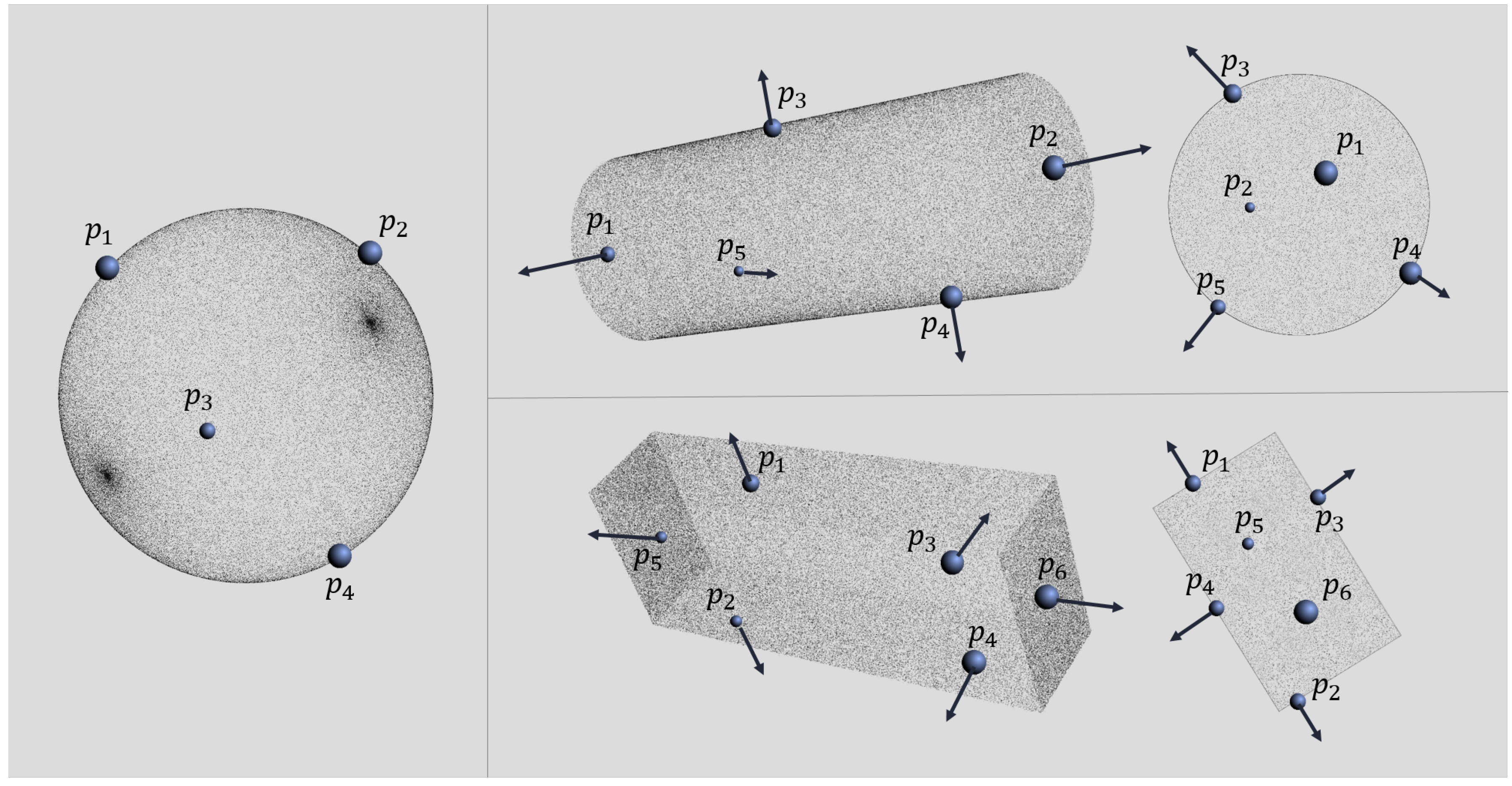
3.1. Representation Scheme

A primitive in a 3D scene is unequivocally described by a finite set of parameters that determine its position (the geometric centre, or centroid, henceforth simply referred to as centre), rotation and other geometrical properties. A solution I is thus naturally encoded as a vector of real values representing the primitive parameters. The size of the vector is shape-specific:

Sphere 

Four parameters: three to locate the centre, and one to represent the radius;

Box 

Ten parameters: three to locate the centre, four to describe the orientation (rotations are described using quaternions), and three parameters to encode the width, depth, and height;

Cylinder 

Nine parameters: three to locate the centre, four to describe the orientation, and two parameters to encode the radius and height;

For the sake of clarity, henceforth a distinction will be made between pose parameters which include the position and, when applicable, the orientation, and the size parameters, namely: the radius of the sphere; the width, depth, and height of the box; and the radius and height of the cylinder.

3.2. Fitness Function

The term ‘fitness function’ is adopted from the EA terminology, and is widely used in the wider metaheuristics literature. In the proposed application, the fitness function quantifies the goodness of fit of a primitive shape I to a given point cloud $\mathcal{PC}=\{p_1,\cdots ,p_N\}$ of N elements. The evaluation criterion for the goodness of fit takes into account two factors: the distance $\delta (p_i,I)$ between each of the individual points $p_i\in \mathcal{PC}$ and the surface of the primitive I; and the concordance $NC(p_i,I)$ of the normals, calculated at each point $p_i\in \mathcal{PC}$, and its projection $\pi (p_i,I)$ on the closest surface of the primitive:

$$\mathcal{F}(I,\mathcal{PC})=\frac{1}{N}\sum _{i=1}^N\frac{NC(p_i,I)}{1+{\frac{\delta (p_i,I)}{{\delta }_{max}}}^2}$$

(1)

where the normalisation factor ${\delta }_{max}$ is the distance between the centroid and the outmost element of the PC. Given a point $p_i\in \mathcal{PC}$, the projection $\pi (p_i,I)$ is the closest part of the candidate primitive surface to the point $p_i$. The computation of $\pi (p_i,I)$ is easy for primitive shapes, and it can be computed very efficiently. The calculation of $NC(p_i,I)$ necessitates of a method to calculate the normals to the elements of a PC. If the normals are not known, the reader is referred to the literature [27,28] for a suitable extraction method. The function in Equation (1) is the same for each type of primitive, whilst the concordance of normals $NC(p_i,I)$ and distance $\delta (p_i,I)$ are type-specific.

For a given sphere S, the distance $\delta (p_i,S)$ between an arbitrary point $p_i$ and $I=S$ is computed as:

$$\delta (p_i,S)=|d(p_i,S_c)-S_r|$$

(2)

where the function $d(A,B)$ measures the Euclidean distance between points A and B, and $S_c$ and $S_r$ are respectively the centre and radius of S. For the box and cylinder, $\delta (p_i,I)$ is computed as the distance between point $p_i\in \mathcal{PC}$ and its projection $\pi (p_i,I)$:

$$\delta (p_i,I)=|d(p_i,\pi (p_i,I))|$$

(3)

The concordance of normals $NC(p_i,I)$ is computed using the cosine similarity between the normal $N\left(p_i\right)$ to point $p_i\in \mathcal{PC}$ and the normal $N\left(\pi (p_i,I)\right)$ of its projection on the candidate primitive surface:

$$NC(p_i,I)=max\left(\frac{N\left(p_i\right)·N\left(\pi (p_i,I)\right)}{\parallel N\left(p_i\right)\parallel \parallel N\left(\pi (p_i,I)\right)\parallel },0\right)$$

(4)

where $·$ denotes the dot product between two vectors. Using Equation (4), only normals that agree in direction contribute to the calculation of the goodness of fit.

From Equation (1), it is easy to see that ${\frac{\delta (p_i,I)}{{\delta }_{max}}}^2$ is minimum and equal to zero when the shape fits perfectly the data. In this case, the denominator of Equation (1) is minimum and equal to 1. The numerator is maximum and equal to 1 when the shape fits perfectly the data, and all the normals agree. Hence, the parameter fitting problem consists of maximising the output of $\mathcal{F}(I,\mathcal{PC})$.

3.3. Local Search Operator

Mutation in the EA and the local search in the BA are performed using the same shape modification operator. Each of the parameters $g_i^I$ describing a candidate primitive shape I may be modified in the following way:

$$g_i^I=g_i^I+0.1(u_i-l_i)\rho$$

(5)

where

$$\rho \sim U(-{\delta }^I,{\delta }^I)$$

(6)

is a random sample drawn with uniform probability in the $[-{\delta }^I,{\delta }^I]$ range, $u_i$ and $l_i$ are respectively the upper and lower bound of the i-th parameter, and $i=\{1,\dots ,n\}$. The number n of parameters is equal to four if I is a sphere, ten if it is a box, and nine if it is a cylinder (Section 3.1). Should one parameter $g_i^I$ be modified to a value outside the $[u_i,l_i]$ interval, it will be placed on the closest extreme.

The shape modification procedure works as follows. The first step is to establish which features (centre, orientation, or size) of the shape are to be modified. If the sought primitive is a sphere, all the features (centre and size) are modified with probability $p^f$. If it is a cylinder or a box, only one feature is changed: either the centre, or the orientation, or the size. The probabilities of changing each of the features is given in the left-hand side of

Table 1. Shape modification probabilities. Probabilities marked with an asterisk are mutually exclusive (e.g., either the centre, or the orientation, or the size of a cylinder is changed).

Feature	${\mathit{p}}^{\mathit{f}}$			${\mathit{g}}_{\mathit{i}}^{\mathit{I}}$	${\mathit{p}}^{\mathit{p}}$
	Sphere	Box	Cylinder		Sphere	Box	Cylinder
Centre	1	0.3 *	0.33 *	X	1	0.7	0.7
				Y	1	0.7	0.7
				Z	1	0.7	0.7
Rotation	-	0.3 *	0.33 *	$w_{1}i$	-	0.7	0.7
				$w_{2}j$	-	0.7	0.7
				$w_{3}k$	-	0.7	0.7
				$w_4$	-	0.7	0.7
Size	1	0.4 *	0.33 *	height	-	0.33 *	0.7
				width	-	0.33 *	-
				depth	-	0.33 *	-
				radius	1	-	0.7

.

Once it has been established which features to change, the second step of the procedure is to determine which parameters (the $g_i^I$) are to be changed. Each parameter $g_i^I$ is modified with a probability $p^p$. For each parameter, the mutation probability is given in the right-hand side of Table 1. For example, if the centre of a box is to be changed, each of its X, Y, and Z coordinates will be changed with probability $p^p=0.7$. If a change of orientation is drawn, the four values describing the orientation are all modified with probability $p^p$. Since orientation is expressed in the form of a unit quaternion, the modified quaternion vector is then normalised.

Preliminary tests have shown that in many cases the optimisation process tended first to fit some surfaces of the candidate primitive to the PC (e.g., the four lateral faces of a box), and then to adjust the remaining ones (e.g., the top and bottom faces). This often led the algorithm to become stuck in shape configurations (i.e., local fitness optima) that could not be further optimised with one single modification event. For example, a box of width $\lambda$ that fits a box-shaped PC of width $\lambda +\delta$ perfectly on five faces, is short on the sixth face. One single change of width would very unlikely fit the sixth face to the data, and at the same time would certainly destroy the alignment of the opposite face to the data (if the width modification is applied symmetrically respect to the centre). To avoid this problem the modification procedure keeps one face of the shape fixed. For example, the height of a box or cylinder may be changed keeping the bottom or top face fixed, and modifying the height.

The differences in the way the shape modification procedure is applied to the different shapes reflect the different levels of disruptiveness the procedure has on said shapes.

3.4. The Bees Algorithm

The bees algorithm (BA) is a popular intelligent optimisation technique that found wide application in optimisation problems [29]. Inspired by the honeybees foraging behaviour, it performs multiple simultaneous local searches at different sites of the solution space. The bees algorithm considers candidate solutions as food sources, and employs artificial bees to evaluate their quality (fitness) and exploit the most promising regions of the search space.

The algorithm begins sending $ns$ artificial scout bees to randomly sampled locations (candidate solutions) in the search space. The scout bees evaluate the quality of the food sources where they landed using Equation (1). Each visited solution becomes the centre of a neighbourhood delimited by a hypercube of side $ngh=2{\delta }^I$. The algorithm then enters the main loop, which consists of a number of steps. The first step is called waggle dance, in analogy with the waggle dance behaviour of honey bees where foragers are recruited for harvesting the richest food sources. In this step, the neighbourhoods around the fittest $nb$ solutions visited by the scouts are selected for local search.

The second step is where the simultaneous exploitative searches are performed, that is the neighbourhoods are harvested (local search). Namely, $nre$ forager bees are sent to exploit the neighbourhood of the very best $ne\le nb$ visited solutions, and $nrb\le nre$ foragers are sent to the remaining $nb-ne$ sites. Each forager lands on a food source in the assigned neighbourhood, and evaluates its quality. The landing site of the foragers is determined using the procedure described in Section 3.3. That is, in the local search step the bees algorithm concurrently samples the neighbourhoods around the most promising solutions. The forager that visited the fittest solution within a neighbourhood becomes the new scout, and the centre of the neighbourhood is moved to that solution.

If no forager finds a solution that is fitter than the centre of the neighbourhood, the scout remains unchanged, and the local search is said to stagnate. In this case, the size of the neighbourhood is reduced (neighbourhood shrinking procedure). After $stlim$ consecutive stagnation cycles the neighbourhood is abandoned and the scout is re-initialised at a new randomly picked location in the search space (site abandonment procedure).

Global explorative search (third step) is performed by the remaining $ns-nb$ scouts, which keep on randomly sampling the solution space looking for new promising regions. At the end of one cycle of the main loop, $nb$ scouts mark the neighbourhoods resulting from local search, and $ns-nb$ scouts mark the neighbourhoods found through global search. The algorithm terminates after a given number of iterations returning the best solution found.

For more details on the bees algorithm and its capabilities, the reader is referred to [7,30,31].

3.5. Evolutionary Algorithm

Evolutionary algorithms (EAs) are global search techniques modelled on the process of natural selection of species as described by Darwin, and on the laws of inheritance of traits postulated by Mendel and Wilson [32,33]. In analogy with biology, in EA terminology the vectors encoding the solutions (Section 3.1) are called chromosomes, and their elements (the parameters) are called genes.

The optimisation process is started randomly initialising a population of p candidate solutions. The algorithm then enters the main loop, which consists of a number of steps. In the first step, the fitness of the population is evaluated using Equation (1). In the second step (selection scheme), the population is ranked in decreasing order of fitness, and sampled with replacement to select $p-1$ seeds (parents). Population sampling is done allocating selection probabilities proportionally to the position in the ranking [8]. In the third step (mutation), the $p-1$ selected parents are used to generate $p-1$ offspring using Equation (5). The mutation procedure employs the parameter modification operator described in Section 3.3. The main difference between the EA and the bees algorithm in the use of the parameter modification operator is that the former encodes the neighbourhood size (${\delta }^I$) in one extra chromosome, and lets it undergo evolution. The EA thus adapts the scope of the local search using the same evolutionary process used to evolve the solutions. The bees algorithm progressively shrinks ${\delta }^I$ via the neighbourhood shrinking procedure.

A new population is formed from the $p-1$ offspring and the fittest individual of the current population, according to the generational replacement with elitism procedure [8].

The EA used in this study iterates $gen$ cycles (generations) of evaluation, selection, and mutation. Genetic crossover [8] is not implemented; for this reason, and the fact that the mutation width ${\delta }^I$ undergoes evolution, the EA is close to the evolutionary programming approach [8].

3.6. RANSAC

As seen in Section 2, a number of RANSAC implementations were proposed in the literature. The main variations over the standard procedure concerned the use of heuristics for faster execution, rather than changes in the search procedure. Often, the precise algorithmic details of these RANSAC variants were not fully reported, and for this reason the standard procedure was implemented in this study [5]. RANSAC is an iterative process, where one new candidate shape is created and scored every cycle. Each iteration comprises of three primary subroutines.

The first RANSAC subroutine creates a minimal subset $P_{ms}$ of points, where $P_{ms}\subset \mathcal{PC}=\{p_1,\cdots ,p_N\}$ and $ms<N$. The subset $P_{ms}$ contains the minimum number of points needed to fully define a candidate shape. Namely, four points are needed to define a sphere, five to define a cylinder and six to define a box (Figure 2).

For the sphere, all four points are randomly sampled at once, and resampled if they are coplanar. For the cylinder and box, one point is picked from the PC at a time, and a set of tests are performed to determine if the newly sampled point is on the same or a different shape face to the points already populating $P_{ms}$ (i.e., all normals must be perpendicular or of opposite direction to each other). The newly sampled point is added if it lies on a different face respect to all points in $P_{ms}$, otherwise is discarded. In the case of the box, the goal of the sampling procedure is to have a point on every face. In the case of the cylinder, the goal is to have three points on the cylindrical outer surface, and one point on each of the end faces.

The second RANSAC subroutine defines a candidate primitive shape from $P_{ms}$. The parameters required to fully define a shape are similar to those defined in Section 3.1, with the sole difference of the use of Euler’s angles (i.e., roll, pitch, yaw) instead of quaternions to define orientation. For spherical primitives, the parameters were found using Schmitt’s technique [34]. For cylinders and boxes, the orientation of the shape is found using the normals to two of the points in $P_{ms}$ (once the orientation of two perpendicular faces is found, the third dimension can be retrieved from the right-hand rule). After the orientation of the candidate shape is found, the size is determined from the whole set of points in $P_{ms}$ (pairs of points in $P_{ms}$ on opposite faces delimit the boundaries of the candidate shape). Finally, the centre is calculated from the reconstructed shape.

The third and final step is to score the candidate primitive shape. The score is calculated as follows:

$$Score\left(I\right)=\sum _{i=1}^{N}min\{dist(p_i,I),ϵ\}$$

(7)

where N is the number of points in the PC, $\delta (p_i,I)$ is the shortest distance between $p_i$ and the surface of the candidate shape I, and $ϵ$ is the approximation tolerance. In the RANSAC implementation used in this paper $ϵ=0.3$. A perfectly fitting shape scores zero.

4. Experimental Method

The performance of the bees algorithm, the EA, and RANSAC was evaluated on three data sets, using a purpose-built error function. This function is different from the goodness of fit function used in the individual algorithms, and this guarantees an unbiased evaluation of the results. For each data set, forty independent runs of each algorithm were performed, and the results statistically analysed. The three data sets are available at the following GitHub repository: https://github.com/lucabaronti/BA-Primitive_Fitting_Dataset.

4.1. Data Sets Used

Each data set comprised of 591 3D models of ${10}^3$ data points each. Each model represented one primitive shape (sphere, box, or cylinder) of different proportions and orientation. Namely, each data set was composed of:

• 181 individual models of spheres. where the radius was varied from 1 to 10 units in steps of 0.05;
• 220 individual models of boxes, where the width, height and depth were varied from 1 to 10 units in steps of 1, and took all possible combinations of these levels (full factorial design). The orientation was randomly determined;
• 190 individual models of cylinders, where the radius was varied from 0.5 to 5 units in increments of 0.25, the height from 1 to 10 units in steps of 1, and radius and height took all possible combinations of these levels (full factorial design). The orientation was randomly determined;

The centre of the shapes was set at the origin. Each PC was created first forming and rotating the primitive shape, and then uniformly sampling ${10}^3$ data points from its surface. The three data sets differed for the amount of noise (error, see Figure 1) in the sampling of the points. Namely:

• Clean set: there is no error, the data points lie exactly on the surface of the primitive shape;
• Error set: the position of each point was randomly perturbed with uniform probability within a 0.1 unit radius;
• Double error: the position of each point was randomly perturbed with uniform probability within a 0.2 unit radius;

In the tests, it is assumed that the type of sought shape is known, and the goal is to find the shape size and orientation. That is, each algorithm is run three times on each data set, each time to fit one specific kind of shape. Each time an algorithm is run on one data set, it is shown only the subset of shapes that needs to be fitted: for example, if the algorithm is required to find the size and orientation of cylinders in the clean data set, only the subset of 190 cylinder models will be used.

4.2. Error Evaluation Function

The best scoring solution F found by an algorithm in a $PC$ (i.e., the found shape) is compared with the real shape I, namely the reference shape used to generate said $PC$.

A fair evaluation of the solutions needs to take into account several issues. First, it involves the comparison of parameters of mixed units (angle degrees for orientation, linear units for size and position), and thus standard metrics (e.g., Euclidean distance) would not be appropriate. Second, differences in the centre or orientation have a larger impact on the matching of the two shapes (and hence on robotic manipulation) than a comparable offset in the size parameters. Finally, the data sets include shapes with differences in size up to one order of magnitude, and the evaluation function should be invariant to size.

The error evaluation function considers the match and alignment of the three segments corresponding to the height, width, and depth of the F and I shapes. Each of the three segments is placed along one of the principal axes of symmetry of the shape (Figure 3). In the case of the box, the lengths of the three segments correspond to the three size parameters of the solution, in case of the cylinder the length of one segment corresponds to the height and the other two to the diameter of the circular section, in case of the sphere they are all equal to the diameter. If the principal axes are not unique (e.g., the three axes of the sphere), they are aligned with the Cartesian axes of the reference frame.

The error is measured from the overlap between the projection of each segment of F onto the three segments of I. In case of perfect matching and alignment, each segment of F (e.g., the height of a box) will project exactly onto the corresponding segment of I, and on a point (i.e., zero overlapping) onto the other two segments (the width and depth) of I. In case of misalignment or incorrect dimensions of F, the projection of one segment (e.g., the height of a box) will not cover exactly the corresponding segment (the height) of I (Figure 4a), and will be non-zero on the other two segments (the width and depth).

Given a solution F, let us denote as $F^1,F^2$ and $F^3$ its three segments (the width, depth, and height respectively), sorted in decreasing order of length, and as ${\widehat{F}}_j^i$ the projection of the $i^{th}$ segment of F on the $j^{th}$ Cartesian axis, where $j=1$ denotes the X axis, $j=2$ denotes the Y axis, and $j=3$ denotes the Z axis. Likewise, for the three axes of I. Finally, let us denote henceforth as $|A|$ the length of a given segment A.

To simplify the calculations, a rigid transformation is applied to express F and I in a new Cartesian frame that corresponds to the three principal axes of I. Note that now $|{\widehat{I}}_i^i|=|I^i|$ and $|{\widehat{I}}_k^i|=0$$\forall k\ne i$ The error $Err(F,I)$ in the alignment and match of F to I is calculated as follows:

$$Err(F,I)=\underset{i=\{1,2,3\}}{min}\left\{\underset{\begin{array}{c}k=\{1,2,3\}\\ k\ne i\end{array}}{min}\left\{M(F^i,I^i)-E(F^i,I^k)\right\}\right\}$$

(8)

$M(F^i,I^i)$ denotes the matching and alignment of $F^i$ with the corresponding segment $I^i$, and is calculated as the length of the intersection ${\widehat{F}}_i^i\cap {\widehat{I}}_i^i$ (green sub-segment in Figure 4a), minus the sum of the lengths of the non-intersecting parts of ${\widehat{F}}_i^i$ and ${\widehat{I}}_i^i$ (red sub-segments in Figure 4a).

$$M(F^i,I^i)=\frac{|{\widehat{F}}_i^i\cap {\widehat{I}}_i^i|-\left[|{\widehat{F}}_i^i|-|{\widehat{F}}_i^i\cap {\widehat{I}}_i^i|\right]-\left[|{\widehat{I}}_i^i|-|{\widehat{F}}_i^i\cap {\widehat{I}}_i^i|\right]}{|{\widehat{I}}_i^i|}$$

(9)

Note that if the found shape F matches perfectly I, $|{\widehat{F}}_i^i\cap {\widehat{I}}_i^i|=|{\widehat{I}}_i^i|$ ($F^i$ is aligned with $I^i$), all the other terms are equal to zero, and $M(F^i,I^i)=1$. In case of total mismatch, $|{\widehat{F}}_i^i\cap {\widehat{I}}_i^i|=0$ and $M(F^i,I^i)=-\frac{|{\widehat{F}}_i^i|+|{\widehat{I}}_i^i|}{|{\widehat{I}}_i^i|}<-1$.

$E(F^i,I^k)$ denotes the mismatch and misalignment of $F^i$, and is measured as the length of the intersection of its projection with the non-corresponding axes $I^k$ of I. That is:

$$E(F^i,I^k)=\underset{\begin{array}{c}k=\{1,2,3\}\\ k\ne i\end{array}}{max}\left\{\frac{|{\widehat{F}}_k^i\cap {\widehat{I}}_k^k|}{|{\widehat{I}}_k^k|}\right\}$$

(10)

Note that if the found shape F corresponds perfectly to I, $|{\widehat{F}}_k^i\cap {\widehat{I}}_k^k|=0$ for all $i\ne k$ ($F^i$ is aligned with $I^i$), and $E(F^i,I^k)=0$. In case $F^i$ is perpendicular to $I^i$ (total mismatch), $F^i$ will be aligned with one of the $I^k$ and $E(F^i,I^k)=1$.

Equation (9) is equal to zero in case F corresponds to I ($M(F^i,I^i)=1$ and $E(F^i,I^k)=0$), is greater than zero otherwise, and is maximum in case of total mismatch ($M(F^i,I^i)<-1$ and $E(F^i,I^k)=1$). The maximum and minimum operations are meant to penalise the main mismatches in length and alignment, whilst being more forgiving on minor discrepancies.

4.3. Parameters Used

The parameterization of the two metaheuristics has been optimised via extensive trial and error, and is shown in

Table 2. Parameterization of the bees algorithm and avolutionary algorithm.

Evolutionary algorithm
Parameter	Sphere	Box	Cylinder
# Individuals	10	10	25
# Parents	3	3	8
Mutation Rate ($p^f$)	1	1	1
# Iterations	390	900	672
Sampling Coverage	5%	25%	25%
Bees algorithm
Parameter	Sphere	Box	Cylinder
Scout bees ($ns$)	2	3	4
Elite sites ($ne$)	1	1	1
Best sites ($nb$)	2	3	4
Recruited elite ($nre$)	9	10	10
Recruited best ($nrb$)	4	4	6
Stagnation limit ($stlim$)	20	30	25
Initial patch neighbourhood ($ngh$)	0.15	0.5	1
# Iterations	300	500	600
Sampling Coverage	5%	25%	25%

. It is different for each shape type, but the same across the three data sets (noisy, error, double error, Section 4.1). The two metaheuristics have been parameterized so as they sample the same number of solutions in one complete optimisation trial.

5. Results

The five-number summary [35] of the primitive fitting tests is shown for each algorithm in

Table 3. Five-number summary of the primitive fitting results obtained by the evolutionary algorithm, bees algorithm and RANSAC on the three data sets.

Clean
Shape	Algorithm	Min	First quartile	Median	Third quartile	Max
Sphere	Evolutionary algorithm	1.055 × 10−3	8.898 × 10−3	1.410 × 10−2	2.135 × 10−2	8.831 × 10−2
Sphere	Bees algorithm	1.270 × 10−5	1.594 × 10−4	2.585 × 10−4	4.132 × 10−4	1.625 × 10−3
Sphere	RANSAC	0	0	0	0	0
Box	Evolutionary algorithm	8.170 × 10−3	2.517	2.815	3.514	1.217 × 101
Box	Bees algorithm	7.828 × 10−2	1.903	2.353	2.938	1.246 × 101
Box	RANSAC	1.490 × 10−8	2.500	2.714	3.250	7.00
Cylinder	Evolutionary algorithm	8.893 × 10−2	1.954	4.441	8.938	1.071 × 103
Cylinder	Bees algorithm	2.069 × 10−1	1.824	3.709	7.667	1.052 × 103
Cylinder	RANSAC	1.902	2.481	2.696	3.162	1.115 × 102
Single Error
Shape	Algorithm	Min	First quartile	Median	Third quartile	Max
Sphere	Evolutionary algorithm	1.075 × 10−3	9.255 × 10−3	1.435 × 10−2	2.250 × 10−2	1.013 × 10−1
Sphere	Bees algorithm	1.075 × 10−4	1.022 × 10−3	1.690 × 10−3	2.885 × 10−3	3.689 × 10−2
Sphere	RANSAC	3.061 × 10−4	3.462 × 10−3	5.391 × 10−3	9.289 × 10−3	5.755 × 10−2
Box	Evolutionary algorithm	7.724 × 10−3	2.496	2.802	3.517	1.212 × 101
Box	Bees algorithm	3.498 × 10−2	1.872	2.348	2.938	1.167 × 101
Box	RANSAC	1.175 × 10−2	2.230	2.511	2.955	7.106
Cylinder	Evolutionary algorithm	8.816 × 10−2	1.954	4.478	9.032	1.054 × 103
Cylinder	Bees algorithm	1.141 × 10−1	1.813	3.758	7.711	1.140 × 103
Cylinder	RANSAC	6.959 × 10−2	2.222	2.426	2.779	1.082 × 103
Double Error
Shape	Algorithm	Min	First quartile	Median	Third quartile	Max
Sphere	Evolutionary algorithm	9.426 × 10−4	9.769 × 10−3	1.522 × 10−2	2.319 × 10−2	1.270 × 10−1
Sphere	Bees algorithm	2.037 × 10−4	1.838 × 10−3	3.140 × 10−3	5.610 × 10−3	7.257 × 10−2
Sphere	RANSAC	5.078 × 10−4	6.800 × 10−3	1.066 × 10−2	1.776 × 10−2	1.077 × 10−1
Box	Evolutionary algorithm	1.795 × 10−2	2.482	2.768	3.471	1.210 × 101
Box	Bees algorithm	8.176 × 10−2	1.899	2.351	2.991	1.200 × 101
Box	RANSAC	2.545 × 10−2	2.081	2.425	2.843	7.272
Cylinder	Evolutionary algorithm	8.970 × 10−5	1.984	4.514	9.347	1.095 × 103
Cylinder	Bees algorithm	1.251 × 10−1	1.880	3.884	8.076	1.170 × 103
Cylinder	RANSAC	1.562 × 10−1	2.070	2.339	2.693	8.833 × 102

for the clean, error, and double error data sets. The five-number summary is a popular set of robust descriptive statistics that provide the central tendency (median), spread (first and third quartile), and range (minimum and maximum) of the distribution of the results.

In terms of accuracy (median value), the bees algorithm performed particularly well on spheres and boxes, where it obtained errors that were smaller than or comparable to the errors obtained by the EA and RANSAC. On cylinders, although the performances of the bees algorithm and RANSAC were close, the latter obtained the best results.

In terms of consistency (first and third quartiles), RANSAC and the bees algorithm performed comparably on boxes and spheres, whilst RANSAC was clearly superior in the fitting of cylinders.

Overall, the EA was the least accurate and consistent of the three algorithms on all data sets and shapes. All the three algorithms proved robust to error, as their performances on the clean data set are indistinguishable from those obtained on the error and double error data sets.

6. Discussion

The state-of-the-art RANSAC algorithm is widely used because of its ability to precisely fit shapes to PC models. The performance of RANSAC in terms of accuracy and speed strongly depends on a number of ad hoc assumptions like the tolerance threshold. The results presented in Section 5 proved that the bees algorithm is able to obtain results of quality (accuracy and consistency) comparable to those obtained using RANSAC, without the need for domain-specific assumptions. Compared to another state-of-the-art metaheuristics (EA), the bees algorithm was able to fit primitive shapes to PC scenes with greater accuracy and consistency.

Although the bees algorithm had not been optimised for speed, single shape fitting times were in the order of fractions of a second (on average, a single primitive was fitted to a shape in $\approx 0.6$ s on an Intel i7 2.8GHz processor.), and thus fully compatible with real-time operations. If needed, optimisation and parallelisation would boost the efficiency of the bees algorithm.

The bees algorithm showed also considerable robustness to error, which simulated imprecision in laser scanning devices. Overall, the tests presented in this paper offer a first indication of the capability of the bees algorithm to solve effectively and efficiently the primitive fitting problem, with performances comparable to or better than the state-of-the-art. The strength of the bees algorithm is that it does not need any assumption to be made on the model.

It should also be noted that in the comparison of Section 5 RANSAC was advantaged by the initialisation subroutine. Candidate shapes were in fact initialised with points sampled from the PC, making sure that these points lied on opposite sides of the shape Figure 2. It is arguable that a similar seeding of the candidate solutions could boost the performance of the bees algorithm and the EA.

7. Conclusions

In this paper the ability of the bees algorithm to solve the primitive fitting problem was evaluated. The performance of the bees algorithm was tested on the recognition of three kinds of primitive shapes from artificially generated data sets, and compared to the performance of the state-of-the-art RANSAC algorithm and the EA metaheuristics.

The tests showed that the bees algorithm is more precise and consistent than the EA, and performs with comparable accuracy to and consistently as RANSAC. Although not optimised for speed, the efficiency of the bees algorithm was compatible with real-time applications. Like the other two algorithms, the bees algorithms showed considerable robustness to error in the PC models. This result indicates the suitability of the bees algorithm to handle data from noisy and imprecise sensors.

The main advantage of the bees algorithm over techniques like RANSAC is that it doesn’t need ad hoc assumptions to be made on the models. In particular, RANSAC is sensitive to the choice of the error tolerance threshold, which usually requires careful optimisation for top performance. RANSAC needs also a seeding procedure to generate the candidate shape, which is then scored on its fit to the rest of the PC model. In its present implementation, the bees algorithm does not need any seeding of the candidate solutions.

The tests performed in this work featured only PCs representing single objects. Further tests will be carried out to investigate the ability of the bees algorithm to recognise multiple and possibly different shapes in a scene. One possible scheme would be to carry out parallel searches for different shapes, for example one kind of shape for each neighbourhood. At the end, the best fitting shapes for each region of the scene would be retained. The performance of the bees algorithm on partial shapes needs also to be evaluated, in order to assess its suitability to cluttered environments.

Finally, the current implementation of the bees algorithm is also extendable to other kinds of shapes, as long as a measure of the distance of the points from the candidate shape can be expressed, and the concordance of the normals can be evaluated. Further work should include validation of the proposed algorithm on more shapes and less geometrically regular objects.

References

1. Bjorkman, M.; Bekiroglu, Y.; Hogman, V.; Kragic, D. Enhancing visual perception of shape through tactile glances. In Proceedings of the 2013 IEEE/RSJ International Conference on Intelligent Robots and Systems (IROS), Tokyo, Japan, 3–7 November 2013; pp. 3180–3186. [Google Scholar]
2. Mavrakis, N.; Stolkin, R.; Baronti, L.; Kopicki, M.; Castellani, M. Analysis of the inertia and dynamics of grasped objects, for choosing optimal grasps to enable torque-efficient post-grasp manipulations. In Proceedings of the 2016 IEEE-RAS 16th International Conference on Humanoid Robots (Humanoids), Cancun, Mexico, 15–17 November 2016; pp. 171–178. [Google Scholar]
3. Spiers, A.J.; Liarokapis, M.V.; Calli, B.; Dollar, A.M. Single-grasp object classification and feature extraction with simple robot hands and tactile sensors. IEEE Trans. Haptics 2016, 9, 207–220. [Google Scholar] [CrossRef] [PubMed]
4. Levine, M.D.; Levine, M.D. Vision in Man and Machine; McGraw-Hill: New York, NY, USA, 1985; Volume 574. [Google Scholar]
5. Bolles, R.C.; Fischler, M.A. A RANSAC-Based Approach to Model Fitting and Its Application to Finding Cylinders in Range Data. In Proceedings of the IJCAI, Vancouver, BC, Canada, 24–28 August 1981; Volume 1981, pp. 637–643. [Google Scholar]
6. Mukhopadhyay, P.; Chaudhuri, B.B. A survey of Hough Transform. Pattern Recognit. 2015, 48, 993–1010. [Google Scholar] [CrossRef]
7. Pham, D.T.; Castellani, M. The bees algorithm: modelling foraging behaviour to solve continuous optimization problems. Proc. Inst. Mech. Eng. Part J. Mech. Eng. Sci. 2009, 223, 2919–2938. [Google Scholar] [CrossRef]
8. Fogel, D.B. Evolutionary Computation: Toward a New Philosophy of Machine Intelligence; John Wiley & Sons: Hoboken, NJ, USA, 2006; Volume 1. [Google Scholar]
9. Ballard, D.H. Generalizing the Hough transform to detect arbitrary shapes. Pattern Recognit. 1981, 13, 111–122. [Google Scholar] [CrossRef]
10. Dalitz, C.; Schramke, T.; Jeltsch, M. Iterative hough transform for line detection in 3D point clouds. Image Process. Line 2017, 7, 184–196. [Google Scholar] [CrossRef]
11. Khoshelham, K. Extending generalized hough transform to detect 3d objects in laser range data. In Proceedings of the ISPRS Workshop on Laser Scanning and SilviLaser 2007, Espoo, Finland, 12–14 September 2007. [Google Scholar]
12. Rabbani, T.; Van Den Heuvel, F. Efficient hough transform for automatic detection of cylinders in point clouds. Isprs Wg Iii/3, Iii/4 2005, 3, 60–65. [Google Scholar]
13. Roth, G.; Levine, M.D. Extracting geometric primitives. CVGIP: Image Underst. 1993, 58, 1–22. [Google Scholar] [CrossRef]
14. Sveier, A. Primitive Shape Detection in Point Clouds. Master’s Thesis, Norwegian University of Science and Technology, Trondheim, Norway, 2016. [Google Scholar]
15. Schnabel, R.; Wahl, R.; Klein, R. Efficient RANSAC for point-cloud shape detection. Comput. Graph. Forum 2007, 26, 214–226. [Google Scholar] [CrossRef]
16. Raguram, R.; Frahm, J.M.; Pollefeys, M. A Comparative Analysis of RANSAC Techniques Leading to Adaptive Real-Time Random Sample Consensus. In Computer Vision—ECCV 2008; Forsyth, D., Torr, P., Zisserman, A., Eds.; Springer: Berlin/Heidelberg, Germany, 2008; pp. 500–513. [Google Scholar]
17. Hast, A.; Nysjö, J.; Marchetti, A. Optimal ransac-towards a repeatable algorithm for finding the optimal set. J. WSCG 2013, 21, 21–30. [Google Scholar]
18. Chum, O.; Matas, J. Optimal Randomized RANSAC. IEEE Trans. Pattern Anal. Mach. Intell. 2008, 30, 1472–1482. [Google Scholar] [CrossRef] [PubMed]
19. Liu, J.; Wu, Z.k. An adaptive approach for primitive shape extraction from point clouds. Optik-Int. J. Light Electron Opt. 2014, 125, 2000–2008. [Google Scholar] [CrossRef]
20. Lutton, E.; Martinez, P. A genetic algorithm for the detection of 2D geometric primitives in images. In Proceedings of the 12th IAPR International Conference on Pattern Recognition, 1994. Vol. 1-Conference A: Computer Vision & Image Processing, Jerusalem, Israel, 9–13 October 1994; Volume 1, pp. 526–528. [Google Scholar]
21. Roth, G.; Levine, M.D. Geometric primitive extraction using a genetic algorithm. IEEE Trans. Pattern Anal. Mach. Intell. 1994, 16, 901–905. [Google Scholar] [CrossRef]
22. Gotardo, P.F.; Bellon, O.R.; Silva, L. Range image segmentation by surface extraction using an improved robust estimator. In Proceedings of the IEEE Computer Society Conference on Computer Vision and Pattern Recognition, Madison, WI, USA, 18–20 June 2003; Volume 2, pp. II–33. [Google Scholar]
23. Ugolotti, R.; Micconi, G.; Aleotti, J.; Cagnoni, S. GPU-based point cloud recognition using evolutionary algorithms. In Proceedings of the European Conference on the Applications of Evolutionary Computation, Granada, Spain, 23–25 April 2014; Springer: Berlin/Heidelberg, Germany, 2014; pp. 489–500. [Google Scholar]
24. Eberhart, R.; Kennedy, J. Particle swarm optimization. In Proceedings of the IEEE International Conference on Neural Networks, Perth, Western Australia, 27 November–1 December 1995; Volume 4, pp. 1942–1948. [Google Scholar]
25. Storn, R.; Price, K. Differential evolution—A simple and efficient heuristic for global optimization over continuous spaces. J. Glob. Optim. 1997, 11, 341–359. [Google Scholar] [CrossRef]
26. Somani, N.; Perzylo, A.; Cai, C.; Rickert, M.; Knoll, A. Object detection using boundary representations of primitive shapes. In Proceedings of the 2015 IEEE International Conference on Robotics and Biomimetics (ROBIO), Zhuhai, China, 6–9 December 2015; pp. 108–113. [Google Scholar]
27. Mitra, N.J.; Nguyen, A. Estimating surface normals in noisy point cloud data. In Proceedings of the Nineteenth Annual Symposium on Computational Geometry, San Diego, CA, USA, 8–10 June 2003; ACM: New York, NY, USA, 2003; pp. 322–328. [Google Scholar]
28. Boulch, A.; Marlet, R. Fast and robust normal estimation for point clouds with sharp features. Comput. Graph. Forum 2012, 31, 1765–1774. [Google Scholar] [CrossRef]
29. Pham, D.T.; Baronti, L.; Zhang, B.; Castellani, M. Optimisation of Engineering Systems With the Bees Algorithm. Int. J. Artif. Life Res. (IJALR) 2018, 8, 1–15. [Google Scholar] [CrossRef]
30. Pham, D.T.; Castellani, M. Benchmarking and comparison of nature-inspired population-based continuous optimisation algorithms. Soft Comput. 2014, 18, 871–903. [Google Scholar] [CrossRef]
31. Pham, D.T.; Castellani, M. A comparative study of the Bees Algorithm as a tool for function optimisation. Cogent Eng. 2015, 2, 1091540. [Google Scholar] [CrossRef]
32. Wilson, E.B.; Wilson, E.B. The Cell in Development and Heredity; Technical report; Macmillan: New York, NY, USA, 1928. [Google Scholar]
33. Ayala, F.J.; Kiger, J.A. Modern Genetics; Benjamin and Cummings: Menlo Park, CA, USA, 1984. [Google Scholar]
34. Alston, M. Evolutionary Algorithm vs. RANSAC for Primitive Shape Fitting. Master’s Thesis, University of Birmingham, Birmingham, UK, 2019. [Google Scholar]
35. Hoaglin, D.C.; Mosteller, F.; Tukey, J.W. Understanding Robust and Exploratory Data Analysis; Wiley: Hoboken, NJ, USA, 2000. [Google Scholar]
Figure 1. (Left) clean point cloud, no noise or error. (Middle) point cloud with error, no noise. (Right) point cloud with noise, no error.
Applsci 09 05198 g001
Figure 2. Four non coplanar points are used to define a sphere (see left). Five points are used to define a cylinder, with one on each end face and three on the outer cylindrical surface (see top right). Six points are used to define a box, one point for each side (see bottom right). Note that the cylinder and box require estimated surface normals to the PC to validate the minimal set of points.
Applsci 09 05198 g002
Figure 3. The found shape F is compared to the real shape I projecting its height, depth, and width onto the height, depth, and width of the real shape.
Applsci 09 05198 g003
Figure 4. Projection of the i t h segment of F ( F i ) onto the j t h segment of I ( I j ); that is, the intersection of the projections of F i and I j onto the j t h Cartesian axis. The green part of the segment marks the match (intersection) of the two projections, the red parts the mismatch. In case of perfect match, the green part will be equal to the length of I j , and there will be no red parts. There are six possible cases of partial or no match between the two axes.
Applsci 09 05198 g004