Abstract
This paper presents a single-camera trilateration scheme which estimates the instantaneous 3D pose of a regular forward-looking camera from a single image of landmarks at known positions. Derived on the basis of the classical pinhole camera model and principles of perspective geometry, the proposed algorithm estimates the camera position and orientation successively. It provides a convenient self-localization tool for mobile robots and vehicles equipped with onboard cameras. Performance analysis has been conducted through extensive simulations with representative examples, which provides an insight into how the input errors and the geometric arrangement of the camera and landmarks affect the performance of the proposed algorithm. The effectiveness of the proposed algorithm has been further verified through an experiment.
1. Introduction
This paper introduces a single-camera trilateration scheme that determines the instantaneous 3D pose (position and orientation) of a regular forward-looking camera, which can be moving, based on a single image of landmarks taken by the camera. It provides a convenient self-localization tool for mobile robots and other vehicles with onboard cameras.
Self-localization is a fundamental problem in mobile robotics. This refers to how a mobile robot localizes itself in its environment. Tremendous effort has been made to study this topic. The approach of this paper is inspired by the principle of trilateration which, given the correspondence of external references, is the most adopted external reference-based localization technique for mobile robots.
Trilateration refers to positioning an object based on the measured distances between the object and multiple references at known positions [1,2], i.e., locating an object by solving a system of equations in the form of:
where p0 denotes the unknown position of the object, pi the known position of the ith reference point, and ri the measured distance between p0 and pi. (Even when more than three references are involved in positioning, we still call it “trilateration” instead of “multilateration”, because “multilateration” has been used to name the positioning process based on the difference in the distances from three or more references [3].)
Equation (1) represents the classical ranging-based trilateration problem which depends on measuring the distances between the target object and references. Existing algorithms include: closed-form solutions which have low time complexity, such as the algebraic algorithm proposed by Fang [4] and Ziegert and Mize [5] which refers to the base plane, that by Manolakis [6] which adapts to an arbitrary frame of reference (a few typos in [6] were fixed by Rao [7]), that by Coope [8] which finds the intersection points of n spheres in Pn based on Gaussian elimination, and the line intersection algorithm proposed by Pradhan et al. [9], as well as the geometric solution developed by Thomas and Ros using Cayley–Menger determinants [2], etc.; and numerical methods which provide optimal estimation by minimizing the residue of (1) in some form, such as least-squares estimation [8,10,11], Taylor-series [12], the extended Kalman filtering (EKF) [13,14,15], linear algebraic techniques [8,16], and particle filtering [17,18], etc. Our work in [19] proposed a closed-form algorithm for the non-linear least-squares trilateration formulation that is dominantly addressed with numerical methods, which provides near optimal estimation with low time complexity. Correspondingly, range sensors, which provide direct distance measurements based on the time of flight of the signals, have been dominantly used in trilateration systems, such as those based on ultrasonic [20,21,22,23,24,25,26,27,28,29,30,31,32,33,34], radio frequency (RF) [4,14,15,17,18,35,36,37,38,39,40,41,42,43,44,45], laser [5], and infrared [46] signals, just to name a few. Existing ranging-based trilateration systems mostly adopt a GPS (Global Positioning System)-like configuration with either “fixed transmitters + onboard receiver” or “onboard transmitter + fixed receivers”. They require installing and maintaining relevant signaling devices in the target environment. The accuracy of the time-of-flight measurement depends on the accuracy of synchronization among the transmitters and receivers. Trilateration for moving objects needs to accommodate the time difference among sequentially received ranging signals and the effect of movement. The signal delay caused by obstacles, which is not easy to detect and filter, is a common source of localization inaccuracy. An onboard ranging-based self-trilateration system, which transmits ranging signals and positions itself based on reflected signals, is highly challenging to realize, due to the difficulty in identifying references from only the reflected signals.
Meanwhile, cameras have become major onboard sensors for autonomous mobile robots in various navigation tasks, due to the comprehensive amount of information contained in images. Correspondingly, vision-based trilateration is considered a natural extension of the classical ranging-based trilateration. Stereovision-based trilateration systems have been proposed [47,48,49]. Compared with ranging-based trilateration which depends on signaling between the separate transmitter and receiver, vision-based trilateration determines the ranges to landmarks from onboard-taken camera images, and thus achieves self-trilateration given the correspondence of landmarks. Vision-based trilateration provides a complementary scheme which naturally avoids some aforementioned common issues with ranging-based trilateration, such as synchronization among signaling devices and obstacle-caused signal delay. Because a camera can capture multiple landmarks at the same time, a camera-based trilateration system can thus obtain simultaneous distance measurements from multiple landmarks. One intrinsic challenge for stereovision is to match the landmark projections in the two simultaneous images, in particular when the numbers of observed landmarks are different in the two images, the two cameras view different subsets of landmarks (which are only partly overlapped), or landmarks are projected close to each other on the same image. Mismatching in landmark projections will result in invalid landmark reconstruction, and hence may cause serious errors in localization. This problem can be avoided if trilateration can be achieved using one camera.
Thus, by comparing it with the ranging-based and stereovision-based trilateration schemes, we feel that single-camera trilateration has certain advantages in the category of trilateration techniques for mobile robots and vehicles. However, there has been a lack of systematic discussion on single-camera trilateration so far, with very limited work using single-camera ranging to assist localization, e.g., as a constraint to correct the odometry for 2D robot self-localization [50]. With the intention to fully explore the capability of single-camera trilateration as an independent 3D self-localization scheme, in this paper we propose a general algorithm for single-camera trilateration that can determine the instantaneous 3D pose of a moving camera from a single image of three or more landmarks at known positions, and give a systematic discussion on the formulation and performance analysis of single-camera trilateration. Minimizing the requirements on the hardware system, the proposed algorithm is based on the classical pinhole model of the regular forward-looking camera. When the camera is fixed on a mobile robot, the self-localization of the camera is equivalent to the self-localization of the robot, where the pose of the camera and that of the robot are different by a fixed camera-robot transformation which can be obtained by the robot hand-eye calibration [51,52]; when the camera is movable on the robot, e.g., pan and tilt, the robot pose can be calculated from the camera pose by incorporating the camera-robot transformation. The proposed scheme extends the classical ranging-based trilateration formulation to encompass the geometry of single-camera imaging and defines an integrated trilateration procedure that fits with the nature of single-camera imaging. It also makes the estimation of the camera orientation a natural part of the complete trilateration process, by taking advantage of the geometric information contained in the image.
As the ranging-based trilateration requires the input of the global positions of reference objects, the camera-based trilateration requires the correspondence between observed landmarks and a map of known landmarks. Focusing on discussing the proposed single-camera trilateration algorithm itself in this paper, we refer to the approaches in the literature [53,54,55,56,57] for the solutions of this correspondence problem. Minimally speaking, the proposed single-camera trilateration algorithm is highly applicable to indoor environments with identity-encoded artificial landmarks, such as shape patterns and color patterns, and outdoor environments with salient natural landmarks, such as uniquely-shaped mountain peaks and buildings. It can also be incorporated into a simultaneous localization and mapping (SLAM) process which generates a map of those distinct landmarks while locating the mobile robot with respect to the map.
We initially came up with the concept of single-camera trilateration and carried out some preliminary work based on simulation in [58]. This current paper will present a fully developed single-camera trilateration algorithm with comprehensive performance analysis. Compared with our preliminary work, the work of this current paper made highly significant and extensive further development. The specific contributions on top of our preliminary work include:
- (1)
- The proposed single-camera trilateration algorithm is fully developed with more systematic derivation and well-adopted notations.
- (2)
- The algorithm is developed with high level of completion. In particular, in the preliminary work, the camera orientation estimation algorithm only estimated the directional vector of the camera optical axis; the current work largely enhances the camera orientation estimation by providing a complete estimation of the 3D rotation matrix of the camera frame relative to the environment frame.
- (3)
- A comprehensive performance analysis of the proposed single-camera trilateration algorithm is carried out. In the preliminary work, the performance analysis of the algorithm considered mainly the effect of the landmark position errors in the environment and image; in the current work, a much more extensive performance analysis is carried out with the consideration of not only the effect of the landmark errors but also that of the errors in camera parameters. Moreover, along with the new camera orientation estimation algorithm, the corresponding performance indices are re-defined, and an enhanced performance analysis is carried out. In addition, the performance analysis in the current work is carried out with a much larger number of simulation data.
- (4)
- An experiment is carefully set up and carried out to further verify the effectiveness of the proposed single-camera trilateration algorithm, and check the estimation error under the combined effect of various input errors. Our preliminary work was simulation-based. The experimental work tests the proposed algorithm in the physical environment, which is a significant addition to the simulation-based performance analysis.
2. Single-Camera Trilateration Algorithm
2.1. Notation and Assumptions
The proposed single-camera trilateration algorithm is derived on the basis of the classical pinhole camera model (Figure 1). Here, XgYgZg denotes the global frame of reference attached to the environment in which the camera is moving, and a vector defined in XgYgZg is labeled with a superscript “g”, e.g., gv; XcYcZc denotes the camera frame with the origin at the optical center p0 and Zc axis pointing along the optical axis from p0 towards the image center q0, and a vector defined in XcYcZc is labeled with a superscript “c”, e.g., cv; UV denotes the image frame with the origin at the upper left corner of the image, and a vector defined in UV is labeled with a superscript “m”, e.g., mv; UVW is the corresponding 3D extension of UV. The vectors in XgYgZg, XcYcZc and UVW are 3-dimensional, while those in UV are 2-dimensional. A position defined in XgYgZg or XcYcZc is in the unit of millimeters, while that defined in UV or UVW is in the unit of pixels.
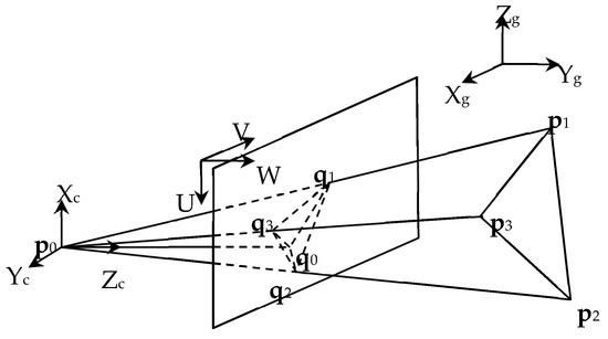
Figure 1.
Pinhole camera model. This figure is adapted from Figure 1 in [58]. (© (2007) IEEE. Reprinted, with permission, from [Liu W.; Zhou Y. Recovering the position and orientation of a mobile robot from a single image of identified landmarks. In Proceedings of 2007 IEEE/RSJ International Conference on Intelligent Robots and Systems, 2007; pp. 1065–1070.]).
In particular, p0 denotes the optical center of the camera, and its positions defined in XgYgZg and XcYcZc are denoted by gp0 and cp0, respectively. q0 denotes the image center (also known as the principal point)—The intersection between the optical axis and image plane (which are perpendicular to each other), and its position defined in UV is denoted by mq0. The distance between p0 and q0 is known as the focal length f. Assuming that there are N landmarks captured by the camera (where N′ ≥ 3 for 3D trilateration according to the principle of trilateration), we denote the reference point of the ith landmark as pi, where i∈{1,2,…,N}, and its positions defined in XgYgZg and XcYcZc are denoted by gpi and cpi, respectively. Moreover, qi denotes the projection of pi on the image plane, and its positions defined in XcYcZc and UV are denoted by cqi and mqi, respectively.
As a necessary input to the proposed single-camera trilateration algorithm, the set of intrinsic parameters of the involved camera can be retrieved from an off-line camera calibration process, a classic topic which has been addressed extensively in computer vision literature such as [59,60,61]. A well-adopted camera calibration toolbox can also be found at [62]. Using the calibration toolbox, we can determine the set of intrinsic camera parameters, including the focal length mf = [fu,fv]T, image center mq0 = [u0,v0]T, and distortion coefficients, as well as their estimation uncertainty. In particular, fu = fDusu, fv = fDv, where f is the physical focal length (mm), Du the pixel size in the U direction (pixel/mm), Dv the pixel size in the V direction, and su the scale factor. It is known that f, Du, Dv and su are in general impossible to calibrate separately [60,61,62]. Therefore, instead of using f, Du, Dv and su separately, we use fu and fv in our algorithm.
The pinhole model is established on the basis of the calibrated camera parameters and corrected image. In the following derivation, we assume that the image distortions have been corrected according to the calibrated distortion coefficients. We also assume that at least three landmarks have been captured, segmented, identified and located at mqi in UV. Relevant image processing techniques can be found in existing literature [59,63,64]. Moreover, we assume that the positions of the involved landmarks in the global frame XgYgZg, gpi, have been retrieved from a map of known landmarks using existing methods [53,54,55,56,57].
The camera position is defined by the position of its optical center p0 in XgYgZg, gp0, and the camera orientation is defined by the rotation matrix of XcYcZc with respect to XgYgZg, gRc. The proposed algorithm will estimate gp0 and gRc, which will be discussed in the following two subsections respectively. The following relationships obtained from the pinhole model will be used in the derivation:
where ui and vi denote the U and V components of mqi respectively.
2.2. Camera Position Estimation
Assuming that N ≥ 3 landmarks are chosen for localizing the camera, we have a system of N independent trilateration equations in XgYgZg in the form of:
which is in fact Equation (1) defined in XgYgZg. In principle, given gpi and ri, one can estimate gp0 by solving Equation (5). Representing the standard ranging-based trilateration problem, Equation (5) can be solved using one of the existing closed-form or numerical algorithms in the literature [2,4,5,6,7,8,9,10,11,12,13,14,15,16,19]. Here, gpi are known as the pre-mapped landmark positions, but ri are yet to be determined.
In order to determine ri, we can write down a system of totally N (N − 1)/2 equations as:
each of which is defined in a triangle ∆p0pipj in XgYgZg according to the law of cosine. Here, θij denotes the vertex angle associated with p0 in ∆p0pipj (which is also known as the visual angle that pipj subtends at p0), and rij the distance between pi and pj. In principle, given rij and cosθij, one can estimate ri by solving Equation (6). At least two general schemes can be adopted to obtain ri:
- (1)
- Solving N equations for N variables: first, choose a subset of N independent equations from Equation (6) which contain N variables {ri|i = 1,…,N}; next, by combining the N equations and eliminating N − 1 variables {ri|i = 2,…,N}, obtain a 2N−1-degree polynomial equation of r12, i.e.,then, solve Equation (7) for r1, and substitute r1 into the chosen N equations to solve for {ri|i = 2,…,N} iteratively. When N = 3, (7) is a 4-degree polynomial equation which can be solved in the closed form. When N > 3, (7) is a polynomial equation of degree 8 or greater. Although it has been proven (by Niels Henrik Abel in 1824) that there cannot be any closed-form formula for such a polynomial equation, a number of numerical algorithms are available, such as Laguerre’s method [65], the Jenkins–Traub method [66], the Durand–Kerner method [67], Aberth method [68], splitting circle method [69] and the Dandelin–Gräffe method [70]. The roots of a polynomial can also be found as the eigenvalues of its companion matrix [71,72,73].
- (2)
- Solving an associated optimization problem: A nonlinear least-squares problem can be formulated to estimate the optimal ri that minimizes the residue of Equation (6), i.e.,where r denotes the vector of {ri|i = 1,…,N}. Search-based optimization algorithms are commonly used to solve this category of problems, including both local optimization algorithms, e.g., the steepest descent method and the Newton–Raphson method (also known as Newton’s method), and global optimization algorithms, e.g., the simulated annealing and the genetic algorithm [74,75,76,77,78].
To solve Equations (6)–(8), we need to know rij and cosθij. Here, , but cosθij are yet to be determined.
In order to determine cosθij, we have the following equation in the triangle ∆p0qiqj in XcYcZc according to the law of cosine:
where denotes the distance between p0 and qi, and denotes the distance between qi and qj. Substituting Equation (4) into Equation (9), we obtain:
where
Since mq0 = [u0,v0]T and mf = [fu,fv]T are determined through camera calibration and mqi are obtained by segmenting the visual landmarks from the image, cosθij can be calculated from Equation (10) directly.
Based on the above derivation, it is clear that the camera can be positioned by reversing the above steps. That is, first calculate cosθij from Equation (10), next estimate ri from Equation (6), and then estimate gp0 from Equation (5).
2.3. Camera Orientation Estimation
Knowing gp0 and the set of gpi, we obtain from Equation (2):
where g∆P is a 3 × N matrix with the ith column as g∆pi = gpi − gp0, and cP is a 3 × N matrix with the ith column as cpi. Here, cpi can be determined by substituting Equation (4) into Equation (3):
where czi can be calculated as
Given g∆P and cP, gRc can in principle be calculated from Equation (11) as
However, due to input errors, such as those in reference positioning, camera calibration and image segmentation, the resulting gRc may not strictly be a rotation matrix. In particular, the orthonormality of the matrix may not be guaranteed. Thus, instead of using Equation (14), we go through the following process to obtain a valid rotation matrix.
We define an optimal approximation of gRc as the one that minimizes the residue of Equation (11), i.e.,
where Tr (M) denotes the trace of the matrix M. Since Tr (M1M2) = Tr (M2M1) for two matrices M1 and M2, we have:
where ADBT is the singular value decomposition of the 3 × 3 matrix cPg∆PT in which A and B are orthogonal matrices and D is an diagonal matrix with non-negative real numbers on the diagonal. Since BTgRcA is an orthogonal matrix and D is a non-negative diagonal matrix, we must have:
and correspondingly
Then, we obtain from Equation (18)
which is guaranteed to be an orthogonal matrix.
Based on the above derivation, it is clear that the camera orientation can be determined by first calculating cpi from Equation (12), next conducting the singular value decomposition of the matrix cPg∆PT, and then getting gRc from Equation (19).
2.4. Algorithm Summary
Following the discussions in the above two subsections, we summarize the proposed single-camera trilateration algorithm as Algorithm 1. It estimates the instantaneous 3D pose of a camera, which can be moving, from a single image of landmarks at known positions. Strictly speaking, Algorithm 1 provides a general framework. In particular, Equation (6) in Step (2) and Equation (5) in Step (3) can be solved by a variety of algorithms specific for those steps, as we pointed out.
| Algorithm 1:Single-Camera Trilateration in P3 |
| Input: The camera parameters mq0 (image center) and mf (focal length), the positions of a set of N ≥ 3 landmarks in XgYgZg, {gpi|i∈Z+, 1 ≤ i ≤ N}, and their corresponding projections in UV, {mqi|i∈Z+, 1 ≤ i ≤ N}. |
| Output: The position gp0 and orientation gRc of the camera in XgYgZg. |
|
3. Performance Analysis
The input to the proposed single-camera trilateration algorithm consists of the global positions of the involved landmarks gpi, their positions in the image mqi, the camera focal length mf and image center mq0. In practice, the uncertainty in camera calibration and inaccuracy of image segmentation cause errors in mf, mq0 and mqi, and imperfect mapping brings errors to gpi. In this section, we analyze the effect of these input errors on the accuracy of the estimation output of the camera position gp0 and orientation gRc.
3.1. Performance Indices
We define an input vector x which contains all the above input parameters, i.e., x = [gpiTmqiTmfT mq0T]T. Then gp0 is a function of x, i.e., . Denoting the actual value and random error of x as and δx respectively, we have . Correspondingly, the actual value and output estimate of gp0 can be written as and , respectively, and the estimation error of gp0 is .
We denote the errors of input quantities gpi, mqi, mf and mq0 as δgpi, δmqi, δmf and δmq0 respectively. Adopting the classical scheme of error analysis used in [2,6], we evaluate the effects of δgpi, δmqi, δmf and δmq0 on δgp0, respectively. For any of these input error vectors (generally denoted as δv), we assume that the vector components are zero-mean random variables and uncorrelated with one another with a common standard deviation δv. We adopt two well-accepted performance indices [2,6], the normalized total bias Bp which represents the sensitivity of the systematic position estimation error to the input error, and the normalized total standard deviation error Sp which represents the sensitivity of the position estimation uncertainty to the input error:
where |a|denotes the norm of a vector a, Tr (M) denotes the trace of a matrix M, E(.) denotes the mean of a random variable, and var(.) denotes the variance of a random variable.
Similar to gp0, gRc is also a function of x, i.e., . To make the presentation consistent, we discuss the orientation estimation error in the vector form, and correspondingly define an error metric of gRc as:
where
in the unit of degrees. Here ni denotes the ith column of gRc which corresponds to the x, y or z directional vector of the camera frame with respect to the global frame. As a result, δgθc shows the angular difference between the actual and erroneous camera orientations. Similar to Equations (20) and (21), we define the corresponding performance indices—the normalized total bias Bθ and the normalized total standard deviation error Sθ as:
where Bθ represents the sensitivity of the systematic orientation estimation error to the input error, and Sθ represents the sensitivity of the orientation estimation uncertainty to the input error.
δgθc = [δθ1 δθ2 δθ3]T,
In the following performance analysis, we will report the variation of Bp, Sp, Bθ and Sθ across the simulated spaces of gp0 under the representative σv values of δgpi, δmqi, δmf and δmq0.
3.2. Simulation Settings
A performance analysis has been conducted on the proposed single-camera trilateration algorithm with representative examples in which a moving camera is localized in P3 based on three landmarks, simulated in Matlab.
In the simulated global frame of reference, the landmarks (reference points) are placed at , and . They form an equilateral triangle on the XY plane, inscribed in a circle centered at the origin of the global frame with a radius of r = 500 length units (Figure 2).
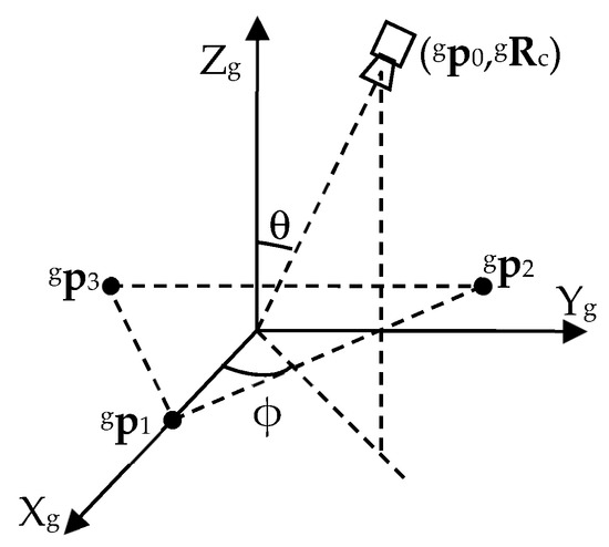
Figure 2.
Simulation settings. This figure is adapted from Figure 3 in [58]. (© (2007) IEEE. Reprinted, with permission, from [Liu W.; Zhou Y. Recovering the position and orientation of a mobile robot from a single image of identified landmarks. In Proceedings of the 2007 IEEE/RSJ International Conference on Intelligent Robots and Systems, 2007; pp. 1065–1070.]).
To study the effect of the geometric arrangement of the camera relative to the landmarks on the performance indices, we let the camera move on a data acquisition sphere S centered at the origin of the global frame with a radius of R, and keep the optical axis of the camera pointing towards the origin. We define a tilt angle θ as the angle between Zg and −n3, and a pan angle ϕ as the angle between Xg and the orthogonal projection of −n3 on the XY plane (Figure 2). To study the effect of the observation distance on the performance indices, we test the algorithm with different values of R. To keep the inscribing circle of the landmarks in the camera field of view all the time, we use R ≥ 3000. It means that the required maximal angle of view is about 19° (corresponding to R = 3000 and θ = 0°), which is a mild requirement met by a large number of lenses. For a specific R, by changing the tilt angle θ and pan angle ϕ, we move the camera on the sphere, and check the variation of the performance indices on the sphere.
The intrinsic camera parameters used in the simulation are obtained by calibrating a real camera (a MatrixVision BlueFox−120 640 × 480 CCD (Charged Coupled Device) grayscale camera with a Kowa 12 mm lens) using the camera calibration toolbox in [62] and a printed black/white checkerboard pattern. In particular, mf = [1627.5609, 1629.9348]T and mq0 = [333.9088, 246.3799]T.
The standard deviations of input errors are chosen mainly according to the calibration results of the above camera and lens. Specifically, using the camera calibration toolbox in [62] to calibrate the camera and lens, we obtained the estimation error for mf as [1.1486, 1.1069]. Since the estimation errors are approximately three times the standard deviation of δmf [62], a representative standard deviation of the δmf components can be taken as σf = 0.4. Meanwhile, the estimation error for mq0 was obtained as [1.9374, 1.5782], which means that a representative standard deviation of the δmq0 components can be taken as σc = 0.6. In addition, we take σp = 25 as a representative standard deviation of the δgpi components, which corresponds to 5% of the base radius r. Besides, σq = 0.5 is taken as a representative standard deviation of the δmqi components based on a conservative estimation of the average image segmentation operation.
For performance analysis, we check the effect of δgpi, δmqi, δmf and δmq0 separately on δgp0 and δgθc. For each of these input error vectors, we assume that the vector components are zero-mean random variables following the corresponding Gaussian distribution and uncorrelated with one another with the same standard deviation; we discretize the data acquisition sphere S with a set of equally gapped θ and ϕ; for each point (θ, ϕ) on S, 10,000 samples of the erroneous input are generated according to the random distribution; the corresponding erroneous output estimates are obtained using the proposed single-camera trilateration algorithm; by comparing the erroneous estimates with the correct camera pose corresponding to (θ, ϕ) on S, the statistics of the output error are generated, and then the performance indices are calculated.
In order to optimally estimate gp0 and ri, we carry out the steps (2) and (3) of Algorithm 1 by solving the corresponding least-squares problems of Equations (5) and (6) respectively. The Newton–Raphson method [74] is used to search for the solutions, which has a sufficient rate of convergence. To avoid being trapped in local minima, for continuous camera position estimation, the previous camera position is used as the initial guess to estimate the current camera position, which guarantees the convergence of the solution to the actual camera position.
3.3. Trends of Performance Indices under Representative Input Error Standard Deviations
To evaluate the impact of δgpi, δmqi, δmf and δmq0 on δgp0 and δgθc, Bp, Sp, Bθ and Sθ are at first estimated with representative input error standard deviations across the data acquisition sphere S with R = 3000. Specifically, Bp(δgpi), Sp(δgpi), Bθ(δgpi) and Sθ(δgpi) are estimated with σp = 25 (Figure 3); Bp(δmf), Sp(δmf), Bθ(δmf) and Sθ(δmf) are estimated with σf = 0.4 (Figure 4); Bp(δmq0), Sp(δmq0), Bθ(δmq0) and Sθ(δmq0) are estimated with σc = 0.6 (Figure 5); and Bp(δmqi), Sp(δmqi), Bθ(δmqi) and Sθ(δmqi) are estimated with σq = 0.5 (Figure 6). Since S is vertically symmetrical to the base plane (XY plane) and horizontally symmetrical to the vertical planes containing the medians of the equilateral base triangle, we only need to display the variation of Bp, Sp, Bθ and Sθ across a patch constrained by θ∈[0°, 90°] and ϕ∈[0°, 60°], while the values of these performance indices at any point on S outside the patch can be obtained according to the symmetry. Each sub-figure in Figure 3, Figure 4, Figure 5 and Figure 6 presents the variation of a performance index, under a specific input error standard deviation, with respect to the observation direction (defined by the tilt angle θ and pan angle ϕ) at a specific distance. Each sub-figure includes one surface plot and one contour plot, both generated using Matlab. The surface plot presents a 3D surface which visualizes the values of the corresponding performance index as heights and colors above a horizontal grid defined by θ and ϕ. The general trend of the performance index’s variation is reflected by the variation in the height and color of the surface. Meanwhile, the contour plot presents a set of isolines (contour lines) at different value levels of the corresponding performance index which varies across θ and ϕ. The contour lines are labeled with the associated values of the performance index in order to provide more numerical details of the variation. To match with the aforementioned data acquisition patch on S, the θ − ϕ grid in each plot is presented in the form of a 2D sector, where the tilt angle of the observation direction θ varies in the radial direction of the sector from 0° to 90° and the pan angle ϕ varies along the arc from 0° to 60°.
For the effect of the landmark position error δgpi:
- (1)
- As shown in Figure 3a, Bp(δgpi) in general decreases as θ increases from 0° towards 90°, although its maximum may not take place exactly at θ = 0°. However, it forms a ridge when θ approaches 90°, which is lower than the crest near θ = 0°. When σp = 25, the ratio between the two peaks is about 6.73.
- (2)
- As shown in Figure 3b–d respectively, Sp(δgpi), Bθ(δgpi) and Sθ(δgpi) in general decrease as θ increases from 0° to 90°, although their maxima may not be exactly at θ = 0°.
For the effect of the imaging-related errors δmqi, δmf and δmq0:
- (1)
- As shown in Figure 4a and Figure 5a, as θ increases from 0°, Bp(δmf) and Bp(δmq0) increase at first to form a high peak, and then decrease generally as θ increases further towards 90°. However, they reach a second, local peak when θ approaches 90°, which is much lower than the first peak. Compared with the first peak, the second peak is far less significant: when σf = 0.4, the ratio between the peaks of Bp (δmf) is about 1095.84; when σc = 0.6, the ratio between the peaks of Bp (δmq0) is about 1525.50.
- (2)
The general decreasing trend of these performance indices towards θ = 90° implies that the camera pose estimation is less sensitive to the input errors as the observations of landmarks are made more parallel and closer to the base plane. Moreover, the non-circular patterns from the contour plots in Figure 3, Figure 4, Figure 5 and Figure 6 reflect the influence of the geometric arrangement of the landmarks.

Figure 3.
Bp(δgpi), Sp(δgpi), Bθ(δgpi) and Sθ(δgpi) with σp = 25 and R = 3000. (a) Surface plot and contour plot of Bp(δgpi); (b) Surface plot and contour plot of Sp(δgpi); (c) Surface plot and contour plot of Bθ(δgpi); (d) Surface plot and contour plot of Sθ(δgpi).
Figure 3.
Bp(δgpi), Sp(δgpi), Bθ(δgpi) and Sθ(δgpi) with σp = 25 and R = 3000. (a) Surface plot and contour plot of Bp(δgpi); (b) Surface plot and contour plot of Sp(δgpi); (c) Surface plot and contour plot of Bθ(δgpi); (d) Surface plot and contour plot of Sθ(δgpi).


Figure 4.
Bp(δmf), Sp(δmf), Bθ(δmf) and Sθ(δmf) with σf = 0.4 and R = 3000. (a) Surface plot and contour plot of Bp(δmf); (b) Surface plot and contour plot of Sp(δmf); (c) Surface plot and contour plot of Bθ(δmf); (d) Surface plot and contour plot of Sθ(δmf).
Figure 4.
Bp(δmf), Sp(δmf), Bθ(δmf) and Sθ(δmf) with σf = 0.4 and R = 3000. (a) Surface plot and contour plot of Bp(δmf); (b) Surface plot and contour plot of Sp(δmf); (c) Surface plot and contour plot of Bθ(δmf); (d) Surface plot and contour plot of Sθ(δmf).


Figure 5.
Bp(δmq0), Sp(δmq0), Bθ(δmq0) and Sθ(δmq0) with σc = 0.6 and R = 3000. (a) Surface plot and contour plot of Bp(δmq0); (b) Surface plot and contour plot of Sp(δmq0); (c) Surface plot and contour plot of Bθ(δmq0); (d) Surface plot and contour plot of Sθ(δmq0).
Figure 5.
Bp(δmq0), Sp(δmq0), Bθ(δmq0) and Sθ(δmq0) with σc = 0.6 and R = 3000. (a) Surface plot and contour plot of Bp(δmq0); (b) Surface plot and contour plot of Sp(δmq0); (c) Surface plot and contour plot of Bθ(δmq0); (d) Surface plot and contour plot of Sθ(δmq0).


Figure 6.
Bp(δmqi), Sp(δmqi), Bθ(δmqi) and Sθ(δmqi) with σc = 0.5 and R = 3000. (a) Surface plot and contour plot of Bp(δmqi); (b) Surface plot and contour plot of Sp(δmqi); (c) Surface plot and contour plot of Bθ(δmqi); (d) Surface plot and contour plot of Sθ(δmqi).
Figure 6.
Bp(δmqi), Sp(δmqi), Bθ(δmqi) and Sθ(δmqi) with σc = 0.5 and R = 3000. (a) Surface plot and contour plot of Bp(δmqi); (b) Surface plot and contour plot of Sp(δmqi); (c) Surface plot and contour plot of Bθ(δmqi); (d) Surface plot and contour plot of Sθ(δmqi).

3.4. Variation of Performance Indices under Variation of Input Error Standard Deviations
To examine the variation of Bp, Sp, Bθ and Sθ under the variation of the input error standard deviations, we compare the values of these performance indices obtained with a set of different values of the input error standard deviations on the data acquisition sphere S with R = 3000. Specifically, Bp(δgpi), Sp(δgpi), Bθ(δgpi) and Sθ(δgpi) are estimated with σp = {25,50,75} (Figure 7); Bp(δmf), Sp(δmf), Bθ(δmf) and Sθ(δmf) are estimated with σf = {0.4,0.6,0.8} (Figure 8); Bp(δmq0), Sp(δmq0), Bθ(δmq0) and Sθ(δmq0) are estimated with σc = {0.6,0.8,1.0} (Figure 9); and Bp(δmqi), Sp(δmqi), Bθ(δmqi) and Sθ(δmqi) are estimated with σq = {0.5,0.7,0.9} (Figure 10). For the convenience of visualization, we compute the mean of each performance index across ϕ at each θ, plot the curve of variation for this mean value with respect to θ, and include the standard deviation across ϕ as the vertical error bar at each θ. Each vertical error bar has a length equal to the standard deviation both above and below the specific mean value at a specific θ. Moreover, to accommodate the large span between the maxima and minima in these performance indices, we plot the data as logarithmic scale for the vertical axis.
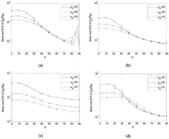
Figure 7.
Comparing Bp(δgpi), Sp(δgpi), Bθ(δgpi) and Sθ(δgpi) with σp = {25, 50, 75} and R = 3000. (a) Variation of Bp(δgpi); (b) Variation of Sp(δgpi); (c) Variation of Bθ(δgpi); (d) Variation of Sθ(δgpi).
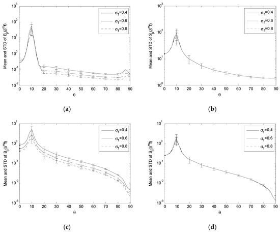
Figure 8.
Comparing Bp(δmf), Sp(δmf), Bθ(δmf) and Sθ(δmf) with σf = {0.4,0.6,0.8} and R = 3000. (a) Variation of Bp(δmf); (b) Variation of Sp(δmf); (c) Variation of Bθ(δmf); (d) Variation of Sθ(δmf).
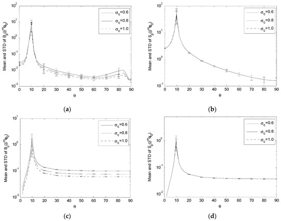
Figure 9.
Comparing Bp(δmq0), Sp(δmq0), Bθ(δmq0) and Sθ(δmq0) with σc = {0.6,0.8,1.0} and R = 3000. (a) Variation of Bp(δmq0); (b) Variation of Sp(δmq0); (c) Variation of Bθ(δmq0); (d) Variation of Sθ(δmq0).
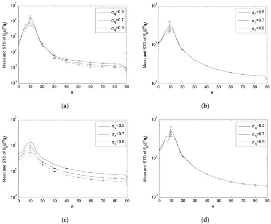
Figure 10.
Comparing Bp(δmqi), Sp(δmqi), Bθ(δmqi) and Sθ(δmqi) with σq = {0.5,0.7,0.9} and R = 3000. (a) Variation of Bp(δmqi); (b) Variation of Sp(δmqi); (c) Variation of Bθ(δmqi); (d) Variation of Sθ(δmqi).
For the effect of δgpi, the simulation results show that, as σp increases,
- (1)
- Bp(δgpi), Sp(δgpi) and Sθ(δgpi) have lower peaks, resulting in flatter variation across S (Figure 7a,b,d);
- (2)
For the effect of δmqi, δmf and δmq0, the simulation results show that, as σq, σf and σc increase,
- (1)
- (2)
The decrease in these performance indices across the whole or portion of S, corresponding to the increase in the input error standard deviations, means that the proposed single-camera trilateration algorithm has a reduced sensitivity to higher input uncertainty under the corresponding geometric arrangements of the camera and landmarks.
3.5. Variation of Performance Indices under Variation of Observation Distance
To examine the variation of Bp, Sp, Bθ and Sθ under the variation of R, we compare the values of these performance indices obtained with representative input error standard deviations on different data acquisition spheres with different radii R = {3000, 4000, 5000} (Figure 11, Figure 12, Figure 13 and Figure 14). For the convenience of comparison, we adopt the same scheme of data plotting as Figure 7, Figure 8, Figure 9 and Figure 10.
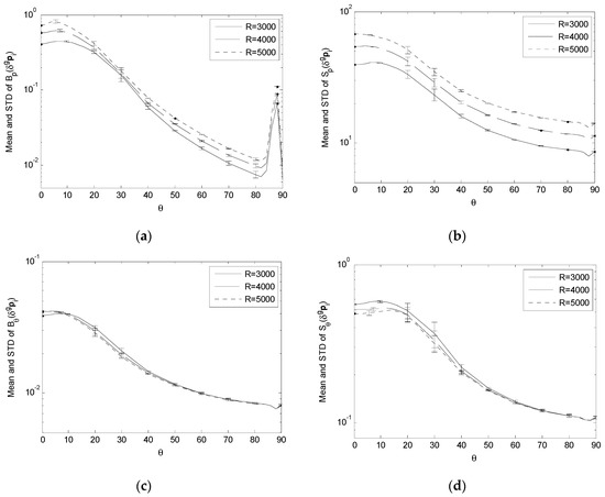
Figure 11.
Comparing Bp(δgpi), Sp(δgpi), Bθ(δgpi) and Sθ(δgpi) with σp = 25 and R = {3000, 4000, 5000}. (a) Variation of Bp(δgpi); (b) Variation of Sp(δgpi); (c) Variation of Bθ(δgpi); (d) Variation of Sθ(δgpi).
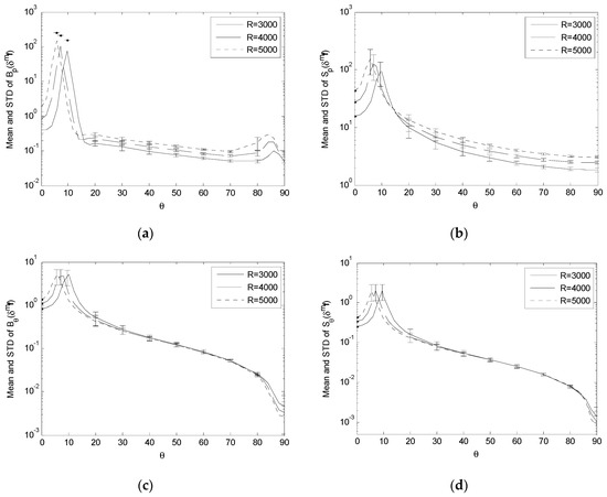
Figure 12.
Comparing Bp(δmf), Sp(δmf), Bθ(δmf) and Sθ(δmf) with σf = 0.4 and R = {3000, 4000, 5000}. (a) Variation of Bp(δmf); (b) Variation of Sp(δmf); (c) Variation of Bθ(δmf); (d) Variation of Sθ(δmf).
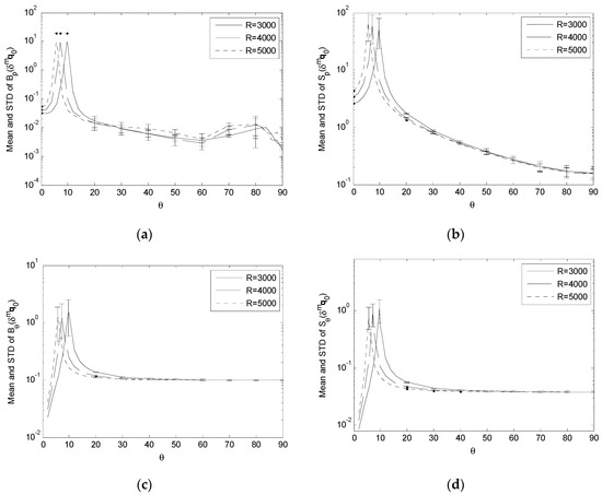
Figure 13.
Comparing Bp(δmq0), Sp(δmq0), Bθ(δmq0) and Sθ(δmq0) with σc = 0.6 and R = {3000, 4000, 5000}. (a) Variation of Bp(δmq0); (b) Variation of Sp(δmq0); (c) Variation of Bθ(δmq0); (d) Variation of Sθ(δmq0).
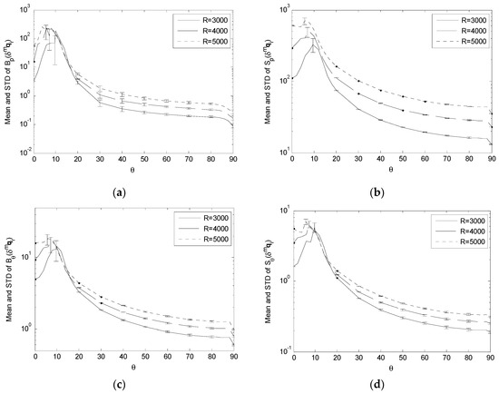
Figure 14.
Comparing Bp(δmqi), Sp(δmqi), Bθ(δmqi) and Sθ(δmqi) with σq = 0.5 and R = {3000, 4000, 5000}. (a) Variation of Bp(δmqi); (b) Variation of Sp(δmqi); (c) Variation of Bθ(δmqi); (d) Variation of Sθ(δmqi).
For the effect of δgpi, the simulation results show that, as R increases,
- (1)
- (2)
- Bθ(δgpi) and Sθ(δgpi) have very small changes and can be considered being essentially independent of the variation of R (Figure 11c,d).
It means that a longer observation distance tends to increase the sensitivity of the positioning bias and uncertainty to the landmark position error, while it has little impact on the corresponding estimation bias and uncertainty of the camera orientation.
For the effect of δmqi, δmf and δmq0, the simulation results show that, as R increases,
- (1)
- (2)
This means that a longer observation distance tends to increase the sensitivity of the positioning bias and uncertainty to the focal length error, and the sensitivity of the positioning and orienting bias and uncertainty to the landmark segmentation error while, except for causing the peaks to shift, it has little impact on the orienting bias and uncertainty due to the focal length error, and the positioning and orienting bias and uncertainty due to the image center error.
3.6. Error-Prone Regions in Performance Indices
Figure 4, Figure 5, Figure 6, Figure 8, Figure 9, Figure 10, Figure 12, Figure 13 and Figure 14 indicate that a sharp high peak consistently appears in Bp, Sp, Bθ and Sθ of δmf, δmqi and δmq0. Each performance index increases to form a high peak as θ increases from 0°, and in general decreases as θ further increases towards 90°. (Though Bp(δmf) and Bp(δmq0) have a second peak later on, it is not so significant as the first peak). The high peak stands out sharply from its neighborhood. On the other side, the crests and transitions in Figure 3, Figure 7 and Figure 11, which show the effect of landmark position errors on the performance indices, are relatively mild.
This high peak is of particular interest. It reflects:
- (1)
- The camera localization algorithm is more sensitive to the errors from the calibration of the camera parameters and segmentation of the landmarks from the image than the errors in positioning the landmarks in the environment.
- (2)
- The neighborhood of a high peak represents a range of camera orientations (relative to the base plane) from which the camera localization is highly sensitive to the errors in camera parameters and image segmentation, resulting in high estimation bias and uncertainty.
Thus, improving the accuracy of camera calibration and image segmentation will help to improve the accuracy of camera localization.
Moreover, knowing the values of θ corresponding to the peaks will help to avoid those error-prone regions in practice. The simulation results reveal that:
- (1)
- (2)
This means that the θ value corresponding to the peaks in the above performance indices is mostly determined by the geometric arrangement of the landmarks and camera.
Although a closed-form estimation of the peak θ value is not available yet, a close approximation can be found through simulations. Specifically in our example where the three reference points define an equilateral triangle, the simulation results show that the peaks occur when the camera is located above the inscribing circle of the base triangle. That is, the θ value corresponding to the peaks is well approximated as:
where r denotes the base radius. This relationship has been verified by comparing the numerically estimated peak locations in these performance indices with θ calculated from Equation (26) (Table 1). Since the θ value at which the peaks appear is consistent across Bp, Sp, Bθ and Sθ of δmf, δmqi and δmq0, only Bp(δmf) is reported here as a representative. Table 1 shows a high consistency between the numerically estimated θ and that calculated from Equation (26). Since the high peaks in these performance indices mean high bias and uncertainty in camera pose estimation, tracking θ at which the observation is made can alert the localization process the error-prone region in practice.

Table 1.
θ Corresponding to the high peak in Bp (δmf) 1.
The above discussion shows that the singular cases represented by the sharp high peaks existing in the plots of performance analysis are related to both the spatial relationship between the camera and landmarks and the usage of camera imaging as the input. Equation (26) provides an effective tool for predicting/estimating potentially singular observation positions. Ultimately, a closed-form representation of the performance indices will lead to analytical analysis of the singular cases. This will be explored in our future work.
4. Experimental Test
An experiment was also carried out to further verify the effectiveness of the proposed single-camera trilateration algorithm, and check the estimation error under the combined effect of various input errors.
A landmark pattern was designed as shown in Figure 15a. It consists of a 679 mm × 679 mm square-shaped checker board pattern and a circle co-centered with the checker board and with a diameter of 679 mm. There are 12 landmark dots equally spaced on the circle, as shown in Figure 15b. The pattern was hung under the ceiling of an indoor experimental space with the base plane parallel to the flat floor. We used the base plane as the XY plane of the global frame of reference, with the Z axis pointing downwards and the center of the pattern as the origin of the frame.
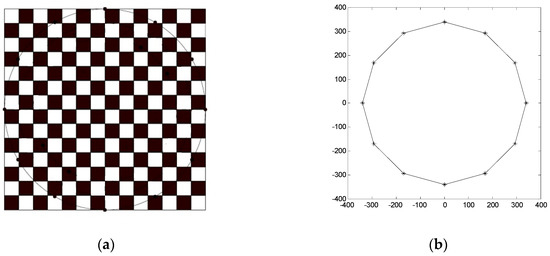
Figure 15.
Landmark pattern used in the experiment: (a) landmark pattern; (b) landmark dot arrangement.
The exact camera, which was calibrated to provide the realistic values of camera parameters for the above simulations, was installed on a Directed Perception PTU-D46-17 controllable pan-tile unit on the top of a Pioneer 3-DX mobile robot (Figure 16) such that the camera was kept on a plane parallel to the base plane at a distance of 1600 mm.
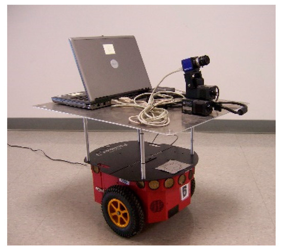
Figure 16.
Onboard experimental system.
We moved the camera (by moving the mobile robot and adjusting the pan-tilt unit) to a number of locations at different observation distances R (which were defined in Section 3.2), one location at one distance. At each location (each R), we adjusted the tilt angle θ and pan angle ϕ (which were defined in Section 3.2) of the camera using the pan-tile unit such that the center of the landmark pattern fell on the image center of the camera, and thus kept the camera oriented towards the landmark pattern. At each location, an image of the landmark pattern was taken by the camera, and stored in the onboard laptop computer.
The collected landmark images were processed after the data acquisition process. Focusing on evaluating the proposed single-camera trilateration algorithm itself, we segmented the landmarks from each image manually after correcting the image distortion. Because the camera optical center is not a physical point on the camera, it is highly difficult, if not impossible, to directly measure the position of the camera optical center and the orientation of the camera optical axis. Thus it is highly difficult to evaluate the localization accuracy of the proposed algorithm according to the golden truth of the camera poses in the global frame. Instead, we chose to compare the camera localization results from the proposed single-camera trilateration algorithm with those obtained from camera calibration (using the camera calibration toolbox in [62]). The camera calibration process calibrated both the intrinsic parameters of the camera, which were input to the proposed algorithm for camera pose estimation, and the extrinsic parameters associated with each calibration image of the checker board pattern, which were used as the reference camera pose estimate to reflect the localization accuracy of the proposed algorithm.
To evaluate the accuracy of the proposed single-camera localization algorithm at different observation distances, we would like to obtain a collection of camera localization results corresponding to different pan angles ϕ at each observation distance R so that we can derive the statistics of localization accuracy at each R, where, as we adjusted the pan/tile unit to align the camera optical axis with the center of the landmark pattern at each R, the tilt angle θ is fixed at each R. Due to the size limitation on the experimental space, it was difficult for us to pan the camera relative to the Z axis of the global frame all around as we kept increasing R. Instead, we took advantage of the design of our landmark pattern. With 12 landmark dots equally spaced on the circle as shown in Figure 15b, we have 12 equally spaced landmark sets labeled as (1, 5, 9), (2, 6, 10), (3, 7, 11), (4, 8, 12), (5, 9, 1), (6, 10, 2), (7, 11, 3), (8, 12, 4), (9, 1, 5), (10, 2, 6), (11, 3, 7) and (12, 4, 8). As mentioned above, at each R (and θ), we took one camera image of the landmark pattern. By using different 3-landmark sets from the same image, we in fact localize the camera corresponding to different ϕ. For example, using landmark set (2, 6, 10) is equivalent to panning the camera from landmark set (1, 5, 9) about the global Z direction by ∆ϕ = 30°. In this way, instead of physically panning the camera, by using different landmark sets to localize the camera, we equivalently obtained the camera localization results corresponding to different ϕ. On the other side, at each R (and θ), the reference camera pose estimate corresponding to each landmark set was obtained by rotating the calibrated camera pose, which was calculated based on the image of the checker board pattern at R (and θ) using the camera calibration toolbox and corresponds to the landmark set (1,5,9), about the global Z axis with a proper ∆ϕ.
The localization results from the proposed single-camera localization algorithm are compared with those from the camera calibration process in Table 2. The calibrated camera pose is used as the reference estimate, and the corresponding calibration error reported by the camera calibration toolbox is presented as the standard deviation of the camera pose calibration. The difference between the camera pose estimated using the proposed algorithm and the calibrated camera pose is recorded as ∆p0 (position estimation difference) and ∆θc (orientation estimation difference), and the mean and standard deviation of these differences are reported. The results in Table 2 show that on average the proposed algorithm attains a localization estimation very close to that attained with camera calibration. The average difference in position estimation is only about 6 mm at an observation distance of R = 4.3 m (corresponding to Rh = 4 m in Table 2), and is smaller with shorter observation distances; the average difference in orientation estimation remains lower than 0.3 degree at an observation distance of R ≤ 4.3 m. While camera calibration cannot be used for real-time localization of a moving camera, the proposed algorithm, which provides a comparable estimation of the camera pose on the go, presents an effective online localization approach for many mobile robot applications. We also notice that the difference in camera position estimation between the two compared methods and the associated standard deviation increase as the observation distance increases. This is mainly because the effective size of the pixels increases as the distance increases. Since the proposed algorithm depends on the segmented landmarks from the same image, the camera positioning error clearly increases as the observation distance and thus the effective pixel size increase; while the camera position estimation error with camera calibration increases much slower, because the calibration process takes advantage of all the images taken at different distances and all the grid corners of the checker board pattern to average out the effect of the increasing effective pixel size. On the other side, the difference in camera orientation estimation between the two compared methods and the associated standard deviation do not appear to be affected as the observation distance increases, due to the cancellation between the effect of the observation distance and that of the effective pixel size. Other factors contributing to the localization error of both methods include the calibration error of the camera intrinsic parameters, and the positioning errors of the landmarks and grid corners due to the printing inaccuracy of the landmark pattern and manual measurement inaccuracy.
Table 2.
Camera pose estimation error—the proposed algorithm versus camera calibration 1.
In addition, to test the speed of the proposed single-camera trilateration algorithm, we implemented a compiled standalone executable (exe file) of the algorithm on a laptop PC with a 1.66 GHz Intel Core 2 CPU, when processing the experimental data. The average estimation speed was about 0.06762 s. In our implementation, the main time-consuming steps were to solve Equations (5) and (6) by using the Newton–Raphson method to search for the solutions of the associated least-squares optimization problems in order to obtain an optimal camera pose estimation.
5. Conclusions and Future Work
This paper has introduced an effective single-camera trilateration scheme for regular forward-looking cameras. Based on the classical pin-hole model and principles of perspective geometry, the position and orientation of such a camera can be calculated successively from a single image of a few landmarks at known positions. The proposed scheme is an advantageous addition to the category of trilateration techniques:
- (1)
- The camera position is trilaterated from multiple simultaneously captured landmarks, which naturally resolves the common concern of the synchronization among multiple distance measurements in ranging-based trilateration systems.
- (2)
- The estimation of the camera orientation becomes an integrated part of the proposed trilateration scheme, taking advantage of the geometrical information contained in a single image of multiple landmarks.
- (3)
- The instantaneous camera pose is estimated from only one single image, which naturally resolves the issue of mismatching among a pair of images in the stereovision-based trilateration.
The proposed single-camera trilateration scheme provides a convenient tool for the self-localization of mobile robots and other vehicles which are equipped with cameras. Depending on the identification of the landmarks involved, the proposed algorithm targets environments with identifiable landmarks, such as indoor and outdoor environments with artificial landmarks, metropolitan environments, and natural environments with distinct landmarks.
The performance of the proposed algorithm has been analyzed in this work based on extensive simulations with a representative set of geometric arrangements among the landmarks and camera and a representative set of input errors. In practice, simulations with the settings of a targeted environment and the input errors of a targeted camera will provide an effective way to predict the algorithm performance in the specific environment and system. The simulation results will provide valuable guidance for the implementation of the proposed algorithm, and facilitate mobile robots to achieve accurate self-localization by avoiding sensitive regions of the performance indices.
Nevertheless, a closed-form solution will further reduce the time complexity of the proposed algorithm, and a closed-form estimation of the performance indices will enable more efficient performance analysis and prediction of the proposed algorithm. As pointed out, existing closed-form solutions can be adopted into the steps (2) and (3) of the proposed framework (Algorithm 1) to solve the 3-landmark case. However, it is challenging to find a closed-form solution which is globally optimal and applies to the general case of 3D trilateration based on more than 3 landmarks. This will be considered in our future work.
Moreover, we target the development of an automatic localization system for mobile robot self-localization based on the proposed single-camera trilateration scheme. The experimental system shown in Figure 16 has provided the necessary onboard hardware for the proposed scheme. Our future work will focus on the development of the software system and supporting vision algorithms.
In addition, over the years of research and development, numerous localization algorithms/approaches in different categories have been proposed in the literature, from deterministic to probabilistic, from ranging-based to image-based. The work of this paper is carried out within the scope of trilateration, with the intention to provide a convenient addition to this category of localization approaches. Meanwhile, the development in other categories of localization approaches are highly significant, e.g., the approaches in the big category of computer vision-based localization [79,80,81]. Our future work on localization may expand into those categories, and comparison study among related approaches is expected.
Author Contributions
Conceptualization of the presented approach, funding acquisition, research supervision, derivation and finalization of the complete algorithm of position and orientation estimation, performance analysis, paper writing, Y.Z.; derivation of the position estimation algorithm of the presented approach, W.L.; experimental study, X.L. and X.Z.
Funding
This research was partly supported by National Science Foundation, grant number1360873.
Conflicts of Interest
The authors declare no conflict of interest.
References
- Borenstein, J.; Everett, H.R.; Feng, L.; Wehe, D. Mobile robot positioning: Sensors and techniques. J. Robot. Syst. 1997, 14, 231–249. [Google Scholar] [CrossRef]
- Thomas, F.; Ros, L. Revisiting trilateration for robot localization. IEEE Trans. Robot. 2005, 21, 93–101. [Google Scholar] [CrossRef]
- Multilateration. Available online: http://en.wikipedia.org/wiki/Multilateration (accessed on 5 December 2019).
- Fang, B. Trilateration and extension to global positioning system navigation. J. Guid. 1986, 9, 715–717. [Google Scholar] [CrossRef]
- Ziegert, J.; Mize, C.D. The laser ball bar: A new instrument for machine tool metrology. Precis. Eng. 1994, 16, 259–267. [Google Scholar] [CrossRef]
- Manolakis, D.E. Efficient solution and performance analysis of 3-D position estimation by trilateration. IEEE Trans. Aerosp. Electron. Syst. 1996, 32, 1239–1248. [Google Scholar] [CrossRef]
- Rao, S.K. Comments on efficient solution and performance analysis of 3-D position estimation by trilateration. IEEE Trans. Aerosp. Electron. Syst. 1998, 34, 681. [Google Scholar]
- Coope, I.D. Reliable computation of the points of intersection of n spheres in Rn. Aust. N. Z. Ind. Appl. Math. J. 2000, 42, C461–C477. [Google Scholar] [CrossRef]
- Pradhan, S.; Hwang, S.S.; Cha, H.R.; Bae, Y.C. Line intersection algorithm for the enhanced TOA trilateration technique. Int. J. Hum. Robot. 2014, 11, 144203. [Google Scholar] [CrossRef]
- Navidi, W.; Murphy, W.S., Jr.; Hereman, W. Statistical methods in surveying by trilateration. Comput. Stat. Data Anal. 1998, 27, 209–217. [Google Scholar] [CrossRef]
- Hu, W.C.; Tang, W.H. Automated least-squares adjustment of triangulation-trilateration figures. J. Surv. Eng. 2001, 127, 133–142. [Google Scholar] [CrossRef]
- Foy, W.H. Position-location solutions by Taylor-series estimation. IEEE Trans. Aerosp. Electron. Syst. 1976, AES-12, 187–194. [Google Scholar] [CrossRef]
- Pent, M.; Spirito, M.A.; Turco, E. Method for positioning GSM mobile stations using absolute time delay measurements. Electron. Lett. 1997, 33, 2019–2020. [Google Scholar] [CrossRef]
- Cho, H.; Kim, S.W. Mobile robot localization using biased chirp-spread-spectrum ranging. IEEE Trans. Ind. Electron. 2010, 57, 2826–2835. [Google Scholar]
- Fujii, K.; Arie, H.; Wang, W.; Kaneko, Y.; Sakamoto, Y.; Schmitz, A.; Sugano, S. Improving IMES localization accuracy by integrating dead reckoning information. Sensors 2016, 16, 163. [Google Scholar] [CrossRef] [PubMed]
- Zhou, Y. An efficient least-squares trilateration algorithm for mobile robot localization. In Proceedings of the 2009 IEEE/RSJ International Conference on Intelligent Robots and Systems, St. Louis, MO, USA, 10–15 October 2009; pp. 3474–3479. [Google Scholar]
- Hsu, C.C.; Yeh, S.S.; Hsu, P.L. Particle filter design for mobile robot localization based on received signal strength indicator. Trans. Inst. Meas. Control 2016, 38, 1311–1319. [Google Scholar] [CrossRef]
- Ullah, Z.; Xu, Z.; Lei, Z.; Zhang, L. A robust localization, slip estimation, and compensation system for WMR in the indoor environments. Symmetry 2018, 10, 149. [Google Scholar] [CrossRef]
- Zhou, Y. A closed-form algorithm for the least-squares trilateration problem. Robotica 2011, 29, 375–389. [Google Scholar] [CrossRef]
- Cheng, X.; Shu, H.; Liang, Q.; Du, D.H. Silent positioning in underwater acoustic sensor networks. IEEE Trans. Veh. Technol. 2008, 57, 1756–1766. [Google Scholar] [CrossRef]
- Ward, A.; Jones, A.; Hopper, A. A new location technique for the active office. IEEE Pers. Commun. 1997, 4, 42–47. [Google Scholar] [CrossRef]
- Priyantha, N.B.; Chakraborty, A.; Balakrishnan, H. The Cricket location-support system. In Proceedings of the 6th ACM/IEEE International Conference on Mobile Computing and Networking, Boston, MA, USA, 6–10 August 2000; pp. 32–43. [Google Scholar]
- Harter, A.; Hopper, A.; Steggles, P.; Ward, A.; Webster, P. The anatomy of a context-aware application. Wirel. Netw. 2002, 8, 187–197. [Google Scholar] [CrossRef]
- Urena, J.; Hernandez, A.; Jimenez, A.; Villadangos, J.M.; Mazo, M.; Garcia, J.C.; Garcia, J.J.; Alvarez, F.J.; De Marziani, C.; Perez, M.C.; et al. Advanced sensorial system for an acoustic LPS. Microprocess. Microsyst. 2007, 31, 393–401. [Google Scholar] [CrossRef]
- Ningrum, E.S.; Hakkun, R.Y.; Alasiry, A.H. Tracking and formation control of leader-follower cooperative mobile robots based on trilateration data. EMITTER Int. J. Eng. Technol. 2015, 3, 88–98. [Google Scholar] [CrossRef][Green Version]
- Petković, M.; Sibinović, V.; Popović, D.; Mitić, V.; Todorović, D.; Đorđević, G.S. Analysis of two low-cost and robust methods for indoor localisation of mobile robots. Facta Univ. Ser. Electron. Energetics 2017, 30, 403–416. [Google Scholar] [CrossRef]
- Dell’Erba, R. Determination of spatial configuration of an underwater swarm with minimum data. Int. J. Adv. Robot. Syst. 2015, 12, 1–18. [Google Scholar] [CrossRef]
- Ureña, J.; Hernández, A.; García, J.; Villadangos, J.M.; Pérez, M.C.; Gualda, D.; Álvarez, F.J.; Aguilera, T. Acoustic local positioning with encoded emission beacons. Proc. IEEE 2018, 106, 1042–1062. [Google Scholar] [CrossRef]
- Park, J.; Lee, J. Beacon selection and calibration for the efficient localization of a mobile robot. Robotica 2014, 32, 115–131. [Google Scholar] [CrossRef]
- Park, J.; Choi, M.; Zu, Y.; Lee, J. Indoor localization system in a multi-block workspace. Robotica 2010, 28, 397–403. [Google Scholar] [CrossRef]
- Kim, S.J.; Kim, B.K. Accurate hybrid global self-localization algorithm for indoor mobile robots with two-dimensional isotropic ultrasonic receivers. IEEE Trans. Instrum. Meas. 2011, 60, 3391–3404. [Google Scholar] [CrossRef]
- Martín, A.J.; Alonso, A.H.; Ruíz, D.; Gude, I.; De Marziani, C.; Pérez, M.C.; Álvarez, F.J.; Gutiérrez, C.; Ureña, J. EMFi-based ultrasonic sensory array for 3D localization of reflectors using positioning algorithms. IEEE Sens. J. 2015, 15, 2951–2962. [Google Scholar] [CrossRef]
- Sanchez, A.; de Castroa, A.; Elvira, S.; Glez-de-Rivera, G.; Garrido, J. Autonomous indoor ultrasonic positioning system based on a low-cost conditioning circuit. Measurement 2012, 45, 276–283. [Google Scholar] [CrossRef]
- Eom, W.; Park, J.; Lee, J. Hazardous area navigation with temporary beacons. Int. J. Control Autom. Syst. 2010, 8, 1082–1090. [Google Scholar] [CrossRef]
- El-Rabbany, A. Introduction to GPS: The Global Positioning System; Artech House: Norwood, MA, USA, 2002. [Google Scholar]
- Ashkenazi, V.; Park, D.; Dumville, M. Robot positioning and the global navigation satellite system. Ind. Robot 2000, 27, 419–426. [Google Scholar] [CrossRef]
- Folster, F.; Rohling, H. Data association and tracking for automotive radar networks. IEEE Trans. Intell. Transp. Syst. 2005, 6, 370–377. [Google Scholar] [CrossRef]
- Bahl, P.; Padmanabhan, V.N. User location and tracking in an in-building radio network. In Microsoft Research Technical Report MSR-TR-99-12; Microsoft Corporation: Redmond, WA, USA, 1999. [Google Scholar]
- Hightower, J.; Borriello, G.; Want, R. SpotON: An indoor 3D location sensing technology based on RF signal strength. In UW CSE Technical Report 2000-02-02; University of Washingtion: Seattle, WA, USA, 2000. [Google Scholar]
- Ahmad, F.; Amin, M.G. Noncoherent approach to through-the-wall radar localization. IEEE Trans. Aerosp. Electron. Syst. 2006, 42, 1405–1419. [Google Scholar] [CrossRef]
- González, J.; Blanco, J.L.; Galindo, C.; Ortiz-de-Galisteo, A.; Fernández-Madrigal, J.A.; Moreno, F.A.; Martínez, J.L. Mobile robot localization based on Ultra-Wide-Band ranging: A particle filter approach. Robot. Auton. Syst. 2009, 57, 496–507. [Google Scholar] [CrossRef]
- Vougioukas, S.G.; He, L.; Arikapudi, R. Orchard worker localisation relative to a vehicle using radio ranging and trilateration. Biosyst. Eng. 2016, 147, 1–16. [Google Scholar] [CrossRef]
- Booma, G.; Umamakeswari, A. An analytical approach for effective location marking of landmine using robot. Res. J. Pharm. Biol. Chem. Sci. 2015, 6, 521–529. [Google Scholar]
- Cotera, P.; Velazquez, M.; Cruz, D.; Medina, L.; MBandala, M. Indoor robot positioning using an enhanced trilateration algorithm. Int. J. Adv. Robot. Syst. 2016, 13, 1–8. [Google Scholar] [CrossRef]
- Reiser, D.; Paraforos, D.S.; Khan, M.T.; Griepentrog, H.W.; Vazquez-Arellano, M. Autonomous field navigation, data acquisition and node location in wireless sensor networks. Precis. Agric. 2017, 18, 279–292. [Google Scholar] [CrossRef]
- Gorostiza, E.M.; Galilea, J.L.L.; Meca, F.J.M.; Monzú, D.S.; Zapata, F.E.; Puerto, L.P. Infrared sensor system for mobile-robot positioning in intelligent spaces. Sensors 2011, 11, 5416–5438. [Google Scholar] [CrossRef]
- Bais, A.; Sablatnig, R. Landmark based global self-localization of mobile soccer robots. Lect. Notes Comput. Sci. 2006, 3852, 842–851. [Google Scholar]
- Zhou, Y.; Liu, W.; Huang, P. Laser-activated RFID-based indoor localization system for mobile robots. In Proceedings of the 2007 IEEE International Conference on Robotics and Automation, Roma, Italy, 10–14 April 2007; pp. 4600–4605. [Google Scholar]
- Spacek, L.; Burbridge, C. Instantaneous robot self-localization and motion estimation with omnidirectional vision. Robot. Auton. Syst. 2007, 55, 667–674. [Google Scholar] [CrossRef]
- Stroupe, A.W.; Sikorski, K.; Balch, T. Constraint-based landmark localization. Lect. Notes Comput. Sci. 2003, 2752, 8–24. [Google Scholar]
- Mao, J.; Huang, X.; Jiang, L. A flexible solution to AX=XB for robot hand-eye calibration. In Proceedings of the 10th WSEAS International Conference on Robotics, Control and Manufacturing Technology, Hangzhou, China, 11–13 April 2010; pp. 118–122. [Google Scholar]
- Shah, M.; Eastman, R.D.; Tsai, H. An overview of robot-sensor calibration methods for evaluation of perception systems. In Proceedings of the Workshop on Performance Metrics for Intelligent Systems, College Park, MD, USA, 20–22 March 2012; pp. 15–20. [Google Scholar]
- Zitova, B.; Flusser, J. Image registration methods: A survey. Image Vis. Comput. 2003, 21, 977–1000. [Google Scholar] [CrossRef]
- De Jong, F.; Caarls, J.; Bartelds, R.; Jonker, P. A two-tiered approach to self-localization. Lect. Notes Comput. Sci. 2002, 2377, 405–410. [Google Scholar]
- Bandlow, T.; Klupsch, M.; Hanek, R.; Schmitt, T. Fast image segmentation, object recognition and localization in a robocup scenario. Lect. Notes Comput. Sci. 2000, 1856, 111–128. [Google Scholar]
- Choi, W.; Ryu, C.; Kim, H. Navigation of a mobile robot using mono-vision and mono-audition. In Proceedings of the IEEE International Conference on Systems, Man, and Cybernetics, Tokyo, Japan, 12–15 October 1999; pp. 686–691. [Google Scholar]
- Atiya, S.; Hager, G.D. Real-time vision-based robot localization. IEEE Trans. Robot. Autom. 1993, 9, 785–800. [Google Scholar] [CrossRef]
- Liu, W.; Zhou, Y. Recovering the position and orientation of a mobile robot from a single image of identified landmarks. In Proceedings of the 2007 IEEE/RSJ International Conference on Intelligent Robots and Systems, San Diego, CA, USA, 29 October–2 November 2007; pp. 1065–1070. [Google Scholar]
- Forsyth, D.A.; Ponce, J. Computer Vision: A Modern Approach; Prentice Hall: Upper Saddle River, NJ, USA, 2002. [Google Scholar]
- Tsai, R.Y. A versatile camera calibration technique for high-accuracy 3D machine vision metrology using off-the-shelf TV cameras and lenses. IEEE J. Robot. Autom. 1987, 3, 323–344. [Google Scholar] [CrossRef]
- Heikkila, J.; Silven, O. A four-step camera calibration procedure with implicit image correction. In Proceedings of the 1997 IEEE Computer Society Conference on Computer Vision and Pattern Recognition, San Juan, PR, USA, 17–19 June 1997; pp. 1106–1112. [Google Scholar]
- Camera Calibration Toolbox for Matlab. Available online: http://www.vision.caltech. edu/bouguetj/calib_doc/ (accessed on 5 December 2019).
- Shapiro, L.G.; Stockman, G.C. Computer Vision; Prentice Hall: Upper Saddle River, NJ, USA, 2001. [Google Scholar]
- Gonzalez, R.C.; Woods, R.E. Digital Image Processing, 3rd ed.; Prentice Hall: Upper Saddle River, NJ, USA, 2007. [Google Scholar]
- Acton, F.S. Numerical Methods that Work; Harper & Row: Manhattan, NY, USA, 1970. [Google Scholar]
- Press, W.H.; Teukolsky, S.A.; Vetterling, W.T.; Flannery, B.P. Numerical Recipes in C++: The Art of Scientific Computing, 2nd ed.; Cambridge University Press: New York, NY, USA, 2002. [Google Scholar]
- Petkovic, M.S.; Carstensen, C.; Trajkovic, M. Weierstrass formula and zero-finding methods. Numer. Math. 1995, 69, 353–372. [Google Scholar] [CrossRef]
- Bini, D.A. Numerical computation of polynomial zeros by means of Aberth’s method. Numer. Algorithms 1996, 13, 179–200. [Google Scholar] [CrossRef]
- Pan, V.Y. Univariate polynomials: Nearly optimal algorithms for numerical factorization and root-finding. J. Symb. Comput. 2002, 33, 701–733. [Google Scholar] [CrossRef]
- Malajovich, G.; Zubelli, J.P. Tangent Graeffe Iteration. Numer. Math. 2001, 89, 749–782. [Google Scholar] [CrossRef]
- Toh, K.; Trefethen, L.N. Pseudozeros of polynomials and pseudospectra of companion matrices. Numer. Math. 1994, 68, 403–425. [Google Scholar] [CrossRef]
- Edelman, A.; Murakami, H. Polynomial roots from companion matrix eigenvalues. Math. Comput. 1995, 64, 763–776. [Google Scholar] [CrossRef]
- Jonsson, G.F.; SVavasis, S. Solving polynomials with small leading coefficients. SIAM J. Matrix Anal. Appl. 2005, 26, 400–414. [Google Scholar] [CrossRef]
- Spall, J.C. Introduction to Stochastic Search and Optimization: Estimation, Simulation, and Control; John Wiley & Sons: Hoboken, NJ, USA, 2005. [Google Scholar]
- Kirkpatrick, S.; Gelatt, C.D.; Vecchi, M.P. Optimization by simulated annealing. Science 1983, 220, 671–680. [Google Scholar] [CrossRef] [PubMed]
- Coley, D.A. An Introduction to Genetic Algorithms for Scientists and Engineers; World Scientific: Hackensack, NJ, USA, 1999. [Google Scholar]
- Back, T.; Fogel, D.B.; Michalewicz, Z. Evolutionary Computation 1: Basic Algorithms and Operators; Institute of Physics: London, UK, 2000. [Google Scholar]
- Back, T.; Fogel, D.B.; Michalewicz, Z. Evolutionary Computation 2: Advanced Algorithms and Operators; Institute of Physics: London, UK, 2000. [Google Scholar]
- Eggert, D.W.; Lorusso, A.; Fisher, R.B. Estimating 3-D rigid body transformations: A comparison of four major algorithms. Mach. Vis. Appl. 1997, 9, 272–290. [Google Scholar] [CrossRef]
- Guan, J.; Deboeverie, F.; Slembrouck, M.; van Haerenborgh, D.; van Cauwelaert, D.; Veelaert, P.; Philips, W. Extrinsic calibration of camera networks using a sphere. Sensors 2015, 15, 18985–19005. [Google Scholar] [CrossRef]
- Penne, R.; Ribbens, B.; Roios, P. An exact robust method to localize a known sphere by means of one image. Int. J. Comput. Vis. 2019, 127, 1012–1024. [Google Scholar] [CrossRef]


© 2019 by the authors. Licensee MDPI, Basel, Switzerland. This article is an open access article distributed under the terms and conditions of the Creative Commons Attribution (CC BY) license (http://creativecommons.org/licenses/by/4.0/).