Abstract
Robust and accurate face alignment remains a challenging task, especially when local noises, illumination variations and partial occlusions exist in images. The existing local search and global match methods often misalign due to local optima without global constraints or limited local representation of global appearance. To solve these problems, we propose a new multi-layer progressive face alignment method that combines global matches for a whole face with local refinement for a given region, where the errors caused by local optima are restricted by globally-matched appearance, and the local misalignments in the global method are avoided by supplementing the representation of local details. Our method consists of the following processes: Firstly, an input image is encoded as a multi-mode Local Binary Pattern (LBP) image to regress the face shape parameters. Secondly, the local multi-mode histogram of oriented gradient (HOG) features is applied to update each landmark position. Thirdly, the above two alignment shapes are weighted as the final result. The contributions of this paper are as follows: (1) Shape initialization by applying an affine transformation to the mean shape. (2) Face representation by integrating multi-mode information in a whole face or a face region. (3) Face alignment by combining handcrafted features with convolutional neural networks (CNN). Extensive experiments on public datasets show that our method demonstrates improved performance in real environments in comparison to some state-of-the-art methods which apply single scale features or single CNN networks. Applying our method to the challenging HELEN dataset, the samples with fewer than 8 mean errors reach 81.1%.
1. Introduction
Face alignment, also called ‘feature point location’, is a process in which a supervised learned model is applied to an input face image to automatically estimate the locations of a set of face landmarks distributed in the eyes, eyebrows, mouth, nose and so on. Face alignment is an important stage in the pipeline of many face analysis applications, such as human computer interactions, expression recognition and identity authentication. Today, it is still a challenging task to automatically and accurately align faces because intrinsic and extrinsic variations exist. The former implies the diversities of the inherent attributes among individuals, such as the shape and texture of eyes, mouth and face. And the latter implies the variations of the image acquisition conditions, such as hair style, glasses, pose, expression and illumination.
Face alignment has a history of 30 years, starting with the early conventional Point Distribution Models, moving to the later Shape Regression methods and to deep learning methods in recent years. Appearance representation is the key to face alignment. The ideal features should reflect only the intrinsic variation, but not be sensitive to the extrinsic variations. Different features can be extracted from a face region or a whole face, which respectively reflect low and high frequency information of a face. Accordingly, the existing face alignment methods can be classified into the two categories: global and local methods.
1.1. The Global Methods
Global methods learn a holistic appearance model to match a new image by optimizing the appearance residual under the current shape parameters. Typical Active Appearance Models (AAM) have been widely used and their extensions mainly focus on fast optimization procedures and texture constraints [1]. Navarathna et al. [2] enhanced the performance for illumination variations by combining Gabor filter responses.
Sun et al. [3] constructed three-level cascade CNN networks to align a face. Trigeorgis et al. [4] extracted the CNN features to input the Recurrent Neural Network (RNN). Zhang et al. [5] combined several cascaded encoder-decoder networks on different resolution images and updated the landmark positions at each stage. Sun et al. [6] regard MLP as a graph transformer network to be embedded into a cascaded regression framework. Wu et al. [7] used a 3-way factorized Restricted Boltzmann Machine (RBM) to build a deep face shape model.
Several multitask deep convolutional networks have been constructed in the cascade manner for jointly achieving face detection, face alignment, pose estimation, and gender recognition [8,9,10]. Head pose is estimated and face variations can be globally restricted by integrating the different deep networks [11]. Three-dimensional information is introduced into the popular CNN networks’ frameworks to extract deep features in face alignment [12,13,14].
The global methods can effectively control and constrain the overall face shape. Their advantage is global optimization and good representation for the whole texture. According to the overall shape, initial error, local noise, partial occlusion and local illumination variation can be tolerated and adjusted to a certain extent. However, because the representation range of the global model depends on the training data, it fails to accurately converge when the input image is dissimilar to the trained appearance. Furthermore, landmarks on the chin and cheeks and other external contours lack rich textures and are relatively isolated, which are somewhat restricted by the global shape, and tend to be attracted to external background noise or other intense gradient regions of a face. When the boundaries between the face region and the background are blurred due to other faces or skin-like objects, although the global optimum can be converged and the face shape can be approximately maintained, the accuracy at the face edge is still very limited.
1.2. The Local Methods
Instead of modeling holistic appearance, local methods merely learn a local texture model for each landmark and restrict all the local decisions according to the global shape to match an image. The earlier Active Shape Models and their improvements have led to the construction of a generative model which measures the variations around a landmark to adjust the model parameters [15,16]. Constrained Local Models (CLMs) describe the local variations by map image, and optimize the parameter set by maximizing the sum of responses [17]. Zadeh et al. [18] use deep CNN networks to produce a local response map which is just like CLM. The independent landmark detectors are trained by learning the discriminative local models, and the landmark positions are updated based on the detection response results [19,20].
A regression function is trained to directly map face appearance to the shape residuals [21,22]. Combining a series of weak regressors in a cascaded manner can progressively reduce the error and achieve higher accuracy [23,24]. The highly discriminative local features are extracted and encoded, followed by the global linear regression [25,26]. Consequently, the local features are integrated under the constraint of the global variation [27,28,29]. Similar approaches combine cascaded regression with the project in order to update the shape parameters [30].
Face alignment under various poses and occlusions is achieved by discriminatively training cascaded deformable part models and optimizing part mixtures [31]. The appearance model combined with head pose tracking by introducing 3D depth information can handle the variations in pose [32,33]. In the composite component graph-matching model [34], the graph structure represents the global attributes and the graph vertex represents the local attribute of key regions. Golnaz et al. [35] built a local block model to realize face detection and alignment by linear regression. Alabort-iMedina et al. [36] combined the holistic model and the part-based model.
The local methods focus on local feature representation and search for a single landmark within the local neighborhood, which can achieve the best performance when the landmark positions are close to the ground-truths. Its advantage is fast computation and good representation for local details. However, because there is no strong mutual constraint between the landmarks across the whole texture, each landmark is aligned separately. A single landmark can be attracted by local noise to drift from the ground-truth. Partial occlusion can cause the loss of local information and detection of the wrong convergence location. Once the initial position is far from the ground-truth, the face shape deforms or drifts as a whole. In sum, this method is greatly influenced by the initial position, image noise and local occlusion, which tend to converge to the local optimum and cause misalignment.
1.3. The Motivation of Our Method
Many researchers have considered combining the two methods in different manners to achieve accurate and stable performance. A straight-forward idea is to estimate the initial positions of the whole face and refine the components locally and independently [37,38]. The local features are used to train a series of random forests for each landmark independently; then, the global features are used to train a random fern to constrain the global shape [39]. The global Net is used to roughly estimate the pose and select the initial shape; then, the local Net is used to predict the shape and pose residuals [40]. The local misalignments are restricted by holistic appearance fitting and the global misalignments are avoided by restricting the local movements [41,42,43]. Duffner et al. [44] predict landmarks by CNN to obtain rough positions and locally refine different parts by several small regional CNNs. Lv et al. [45] use two-stage re-initialization with deep network regressors, in which a coarse face shape is predicted in the global stage and each landmark is estimated respectively in a local stage.
From the view of multi-source information fusion, integrating data from different channels and combining different processing methods can obtain better performance for a specific task. Widely studied emotion recognition investigates multimodal data, including visual, audial, physiological signal, text, and so on. Liang et al. [46] integrate these direct and relative prediction perspectives to obtain excellent performance on an audio-visual emotion recognition benchmark. Tzirakis et al. [47] utilize a CNN to extract robust features from speech, and a deep residual network (ResNet) for the visual modality. Liu et al. [48] demonstrate that the Bimodal Deep AutoEncoder (BDAE) features are effective for emotion recognition. By analyzing the confusing matrices, EEG and eye features can contain complementary information. Felipe et al. [49] propose a novel multimodal emotion recognition system based on visual and auditory information to estimate different emotional states in real affective human robot communication. Ranganathan et al. [50] applied four deep belief network (DBN) models to generate robust multimodal features for emotion classification. Then, convolutional deep belief network (CDBN) models are proposed to learn salient multimodal features of emotions expressions.
The current methods mostly do not jointly consider appearance representation and the alignment strategy. Furthermore, the appropriate features and approaches for the different alignment stages are not carefully selected. The different features from a whole face and a certain region should be respectively extracted based on the different characteristics of the alignment stage. The different scale image information should be combined in different manners as a more descriptive face representation. The current methods mostly reduce the influence of initialization errors by setting multiple initial positions or by direct regression from the face texture. Variations in initial shapes satisfy a certain kind of transformation. The transformation from mean shape to ground-truth should be investigated. The current methods seldom combine traditional handcrafted features with the popular CNN features. Handcrafted features contain more prior knowledge, which helps to represent a face. Accordingly, handcrafted features should be introduced into popular CNN networks as to achieve better performance.
Our research is motivated by the belief that more competitive face alignment results can be obtained if we combine representation information with different scales and apply different methods and approaches for alignment tasks in different phases. Global alignment is more suitable for representing the holistic structure, and therefore, can achieve the global optimum in matching a whole face. Local alignment is good at describing shape details; therefore, it is suitable for refined corrections of given area. In this paper, we build a coarse-to-fine multi-layer progressive face alignment framework that combines global matches and local refinement to achieve better performance, in which the former could constrain the latter and the latter could complement the former.
The face shape is quickly initialized by applying 2D affine transformation to the mean shape, in which the 2D affine parameters are directly estimated. In different alignment stages, our method respectively extracts the global and local features, followed by the different regression approaches. The multi-scale information in an image is combined to form the multi-mode features. The global alignment is performed by regressing the shape parameters from the CNN features on the multi-mode LBP images, instead of on the raw image. A simpler network is enough to achieve the same performance as running a deeper network at the pixel level because we introduce handcrafted features. The local alignment is performed by regressing the landmark position update from the multi-mode HOG features in the local region. Random regression forests can be efficiently performed on parallel architectures, which results in fast calculations. The obtained two shapes are weighted for integration. The experiments indicate that the alignment strategy and the feature representation helps to improve the alignment accuracy while only slightly increasing the computational cost. Our method can not only deal with illumination variations and local noise, but can also compensate for the partial occlusion in an image according to its global information.
1.4. Our Contributions
Our contributions are as follows:
- (1)
- We propose a fast and accurate shape initialization method by applying 2D affine transformation to the mean shape. The corresponding parameters between the mean shape and the ground-truth can be directly estimated by the CNN features around the anchor landmarks.
- (2)
- We propose a global alignment method by feeding new handcrafted features into a popular CNN network to regress the face shape parameters. By introducing prior knowledge, we can enhance the performance compared to methods using the traditional networks.
- (3)
- We propose a local alignment method by feeding multi-mode features into a random regression forest to independently regress and update each landmark position. By introducing the redundant multi-mode information, we can enhance the alignment performance.
- (4)
- We propose a weighted integration method by applying different weight values within each face component to fuse the two alignment results, which allows the final shape to achieve both the global optimum and local refinement.
The rest of this paper is organized as follows. In Section 2, a progressive multi-layer face alignment framework is briefly introduced. In Section 3, more details of the proposed algorithm are given, including different face representation methods, the corresponding alignment approaches and the integration strategy. In Section 4, the comparison experiments on public databases are performed, and the corresponding qualitative and quantitative analysis is presented, followed by a conclusion and discussion in Section 5.
2. Overview of the Proposed Method
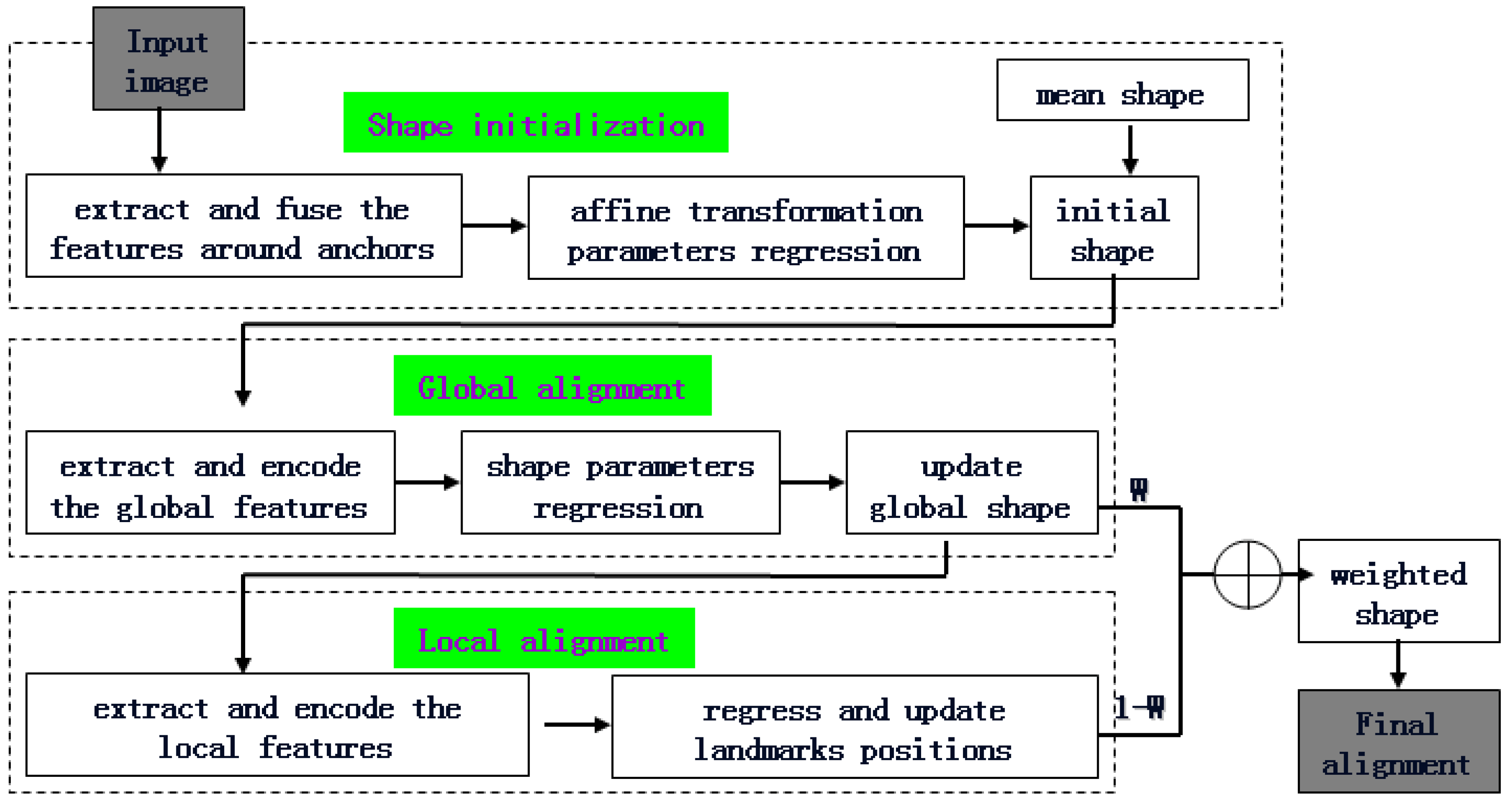
To combine the advantages and overcome the limitations of the global and local methods, in this paper, the global match and local refined correction are integrated and embedded into a three-layer alignment framework. Three layers of pyramid decomposition are performed on the original image. The different features and strategies are applied to the images with different resolutions in each layer. The overview of the proposed framework is shown in Figure 1.
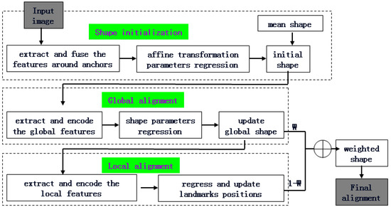
Figure 1.
Overview of the proposed alignment framework.
(1) shape initialization
This procedure is performed on the lowest resolution image. The patches around the anchor landmarks are sent to the CNN networks to regress the 2D affine transformation parameters between the mean shape and the ground-truth. The shape initialization for an input image is realized by applying 2D affine transformation to the mean shape.
(2) global alignment
This procedure is performed on a lower resolution image and the input face shape is obtained from the output of the shape initialization. The magnitude and orientation information from the gradient image is combined as the modified LBP. The modified LBP features with different scales are extracted, concatenated and encoded. Then, an input image is represented as three multi-mode LBP images. Instead of a raw input image, the three multi-mode LBP images are sent to the CNN networks to regress the face shape parameters. Finally, the face shape is globally updated, and global alignment is achieved. Because the multi-mode LBP images contain more distinguishable information than the original pixel-level image, a simpler network is able to achieve the same performance as a deeper network at the pixel level.
(3) local alignment
This procedure is performed on the original resolution image and the input face shape is obtained from the output of the global alignment. The magnitude and orientation information from the gradient image is combined as the representation of a given face region. The multi-mode HOG features around each landmark are extracted, concatenated and encoded. Then, a large number of redundant and more representative local features are obtained and sent to a trained random regression forest. Each landmark position is independently regressed and updated, at which time the shape’s details are further adjusted. Random regression forests can be efficiently performed on parallel architectures, which results in more rapid calculations.
(4) weighted integration
This procedure applies the different weight values within each face component to integrate the global and local alignment shapes. The same weight value is adopted within each component. Then, the final result achieves the global optimum and local refinement jointly.
3. The Multi-Layer Progressive Face Alignment Method
The different alignment strategies and representation features were adopted for each procedure of our alignment framework. Firstly, the 2D affine transformation parameters between the mean shape and the ground-truth were regressed to realize the shape initialization (Section 3.1). Secondly, an input image is encoded as the multi-mode LBP image to regress the face shape parameters by the CNN networks (Section 3.2). Thirdly, the multi-mode HOG features around each landmark are encoded to independently update the landmark position using random regression forests (Section 3.3). Finally, the two alignment shapes are weighted as the final result, which achieves the global optimum and local refinement jointly (Section 3.4).
3.1. Face Shape Initialization
Because the initial position severely affects the final alignment accuracy, fast and accurate shape initialization is very important. In order to reduce the influence of the face initialization, Yan et al. [51] generated multiple hypotheses by randomly shifting and rescaling the face-bounding box. The alignment model is applied to these different initializations, and a series of shape hypotheses are obtained. The parameters in both learn to rank and combine. Burgosartizzu et al. [29] proposed a restart scheme to improve the initialization. Given an image and a number of different initializations, only 10% of the cascade is applied to each. If the variance between their predictions is below a certain threshold, the remaining 90% is applied as usual. Otherwise, the process is restarted with a different set of initializations.
Accurate shape initialization can reduce the error between the mean shape and the ground-truth, which helps to avoid trapping in the local optimum. In this paper, we applied 2D affine transformation to the mean shape to perform shape initialization. The patches around the anchor landmarks are sent to the CNN networks to regress the 2D affine transformation parameters between the mean shape and the ground-truth. Satisfying 2D affine transformation, the global variation of a face can be regarded as a rigid variation caused by scale, translation, and rotation. The 2D affine transformation is expressed as follows:
where and respectively indicate the coordinates of the two shapes, and respectively indicate scale, translation, and rotation. In the six parameters, reflect scale and rotation, and reflect translation. The shape initialization on an input image is realized by applying affine transformation on the mean shape. The six affine transformation parameters can be directly estimated from the local CNN features around the anchor landmarks.
The different patches are cropped around the anchor landmarks in a face image and sent to the corresponding CNN networks. The output of FC layer from each patch is normalized and served as the local features. Then, all the local features are concatenated together in a fusion layer without dimension reduction. The output of the fusion layer is used to regress the affine parameters (as shown in Figure 2).
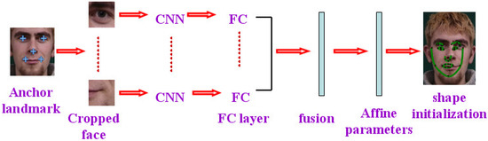
Figure 2.
Face shape initialization based on affine parameters regression.
Although there is a high level of correlation between the different patches, the less local information from a patch cannot intensely affect other information. Because the location relationship between the patches contains the structure information of a whole face, the information from different patches can be combined as face representation. A simpler network with less parameters is applied to learn the efficient features in a single patch. The same network architecture is adopted for different patches, and the parameters of each CNN are trained independently. The architecture used here contains 2 convolutional layers, 2 max-pooling layers, and 1 fully-connected layer with drop out units (as shown in Figure 3). The input cropped face image is normalized to 32 × 32. The number of neurons of the FC layer is 32. The features from all the patches are fused as a vector with 160 dimensions, which is applied to regress the affine transformation parameters.

Figure 3.
CNN networks for each face patch.
Increased convolution stride can compress partial information and reduce network size. In most deep architectures, the pooling layers are just selected from the output of the previous convolution layer. Some researchers considered using the larger convolution stride and expected similar accuracy with reduced computational consumption. Springenberg et al. [52] claim that max-pooling can simply be replaced by increasing the stride without reducing the accuracy on several image recognition benchmarks. Howard et al. [53] applied average pooling before the fully connected layer. Compared with the original networks, overwhelming computing speed and approximate accuracy is obtained. However, the above works just improved computing speedd in image recognition. In contrast, the alignment problem in this paper focuses on improving accuracy rather than speed. Recognition requires the overall features, while alignment requires a precise description for a single landmark. Directly skipping some pixels with a larger stride probably misses some minute and small-scale information on certain face regions, which leads to alignment errors. This paper applies max-pooling instead of larger stride. As one part of a deep learning framework, although max-pooling can also reduce dimension, it is not random sampling but a means of selecting the most prominent features. Furthermore, it has some degree of spatial transformation invariance, and can preserve more texture information.
Feature fusion can enhance the contribution of certain features and reduce the influence of others. Furthermore, the interaction between the more representative features from the different regions can be effectively utilized, which can further improve performance and speed up the convergence. The output of the fusion layer is applied to obtain the six affine parameters by linear regression. The corresponding affine transformation is affected by the mean shape to perform the face shape initialization.
3.2. The Global Alignment Based on Shape Parameters Regression
Multiple features are proposed to represent the whole face, and different features are selected to deal with the specific application. The features can be extracted from the transformed images or the original grayscale images to be applied in face alignment. Tzimiropoulos et al. [54] align the two images by iteratively maximizing their correlation coefficient from the gradient orientations rather than pixel intensities. This process can be extended within the inverse compositional framework, and achieves good performance under occlusions and illumination changes. Taha et al. [55] enhanced the completed Local Binary Pattern (CLBP), an LBP variant with impressive performance on texture classification. Five multi scale color CLBP descriptors are proposed by incorporating different color information into the original CLBP.
In this paper, the magnitude and orientation information from the gradient image is combined as the modified LBP. Then, the multi-mode information of an input image is extracted, concatenated and encoded as the three multi-mode LBP images. Instead of the original grayscale image, the three LBP images are sent to the CNN networks to regress the face shape parameters. Finally, the face shape is globally updated. The multi-mode LBP images contain more distinguishable information than the original pixel-level image. So, a simpler network is enough to achieve the same performance as running a deeper network at the pixel level.
3.2.1. Multi-Mode LBP Images
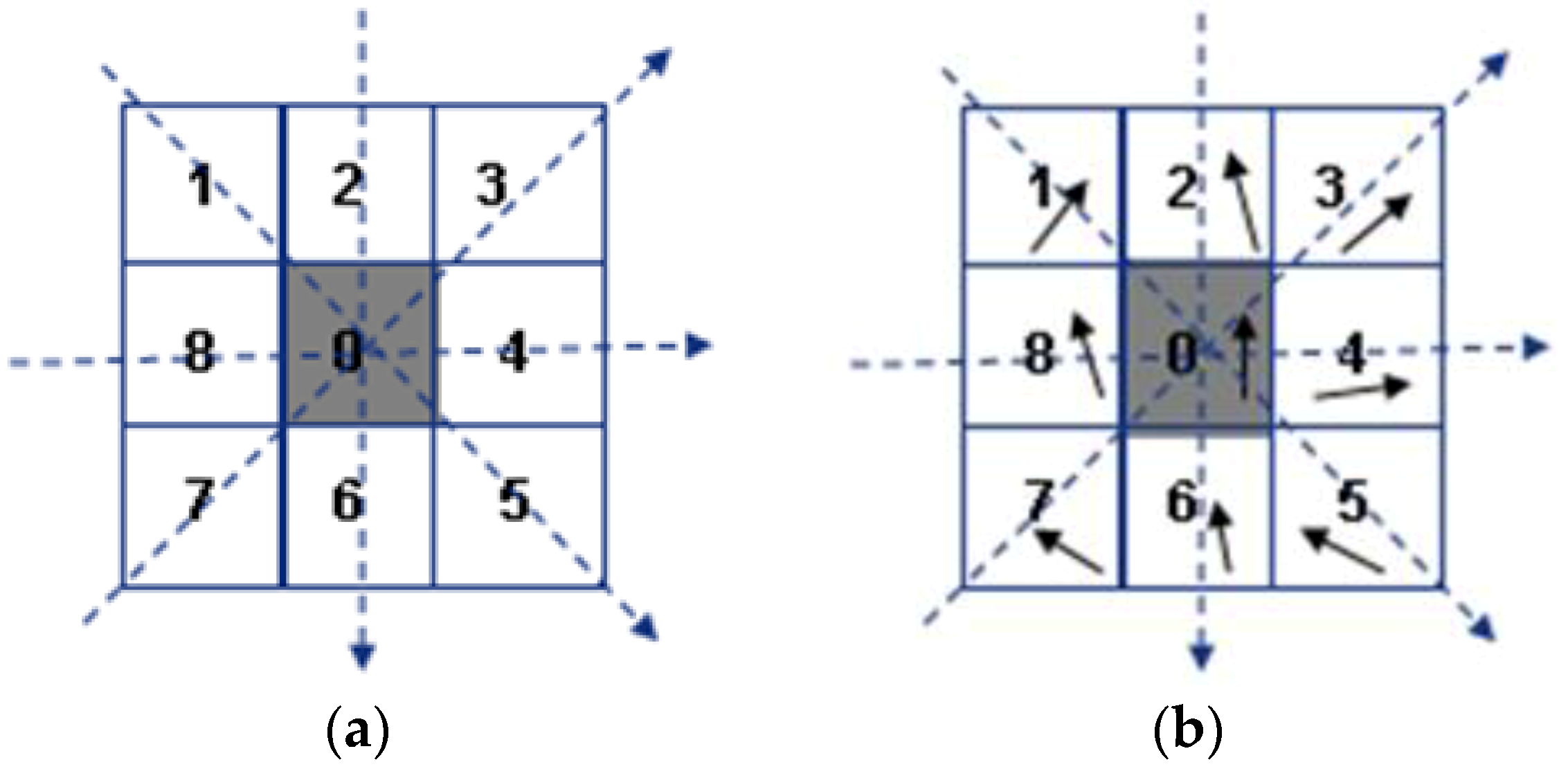
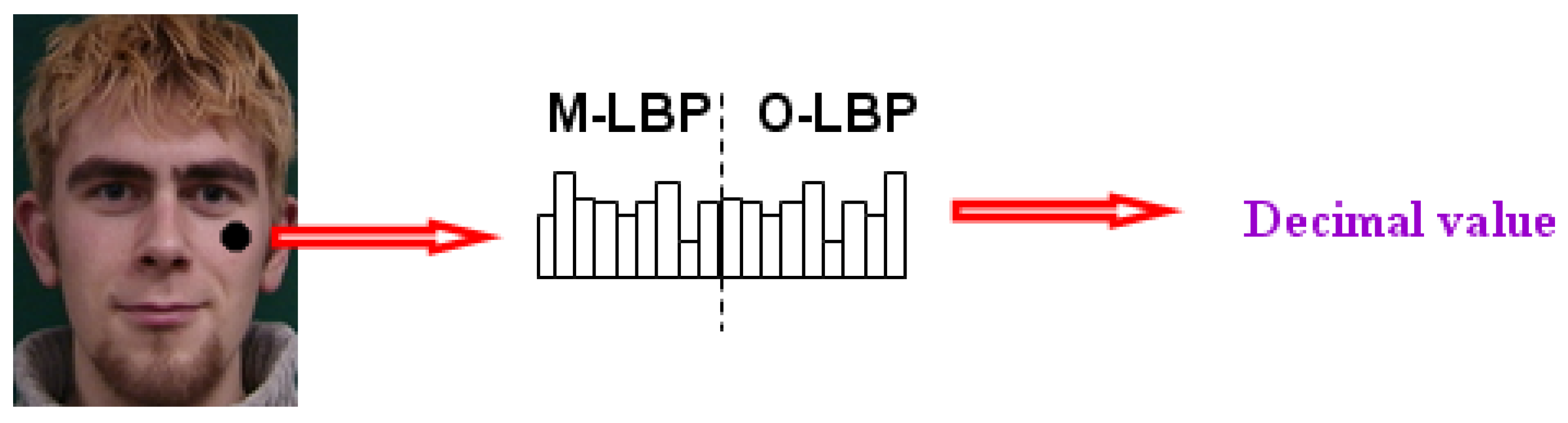
The original LBP only considers pixel-wise difference information. However, the higher-order variation tendency along different directions contains more monotonic properties. The more descriptive information in different pixel responses along a particular direction should be investigated. The second-order variation of gradient magnitude and gradient orientation is extracted to combine as the modified LBP, including M_LBP and O_LBP.
The 3 × 3 neighborhood around the current pixel contains four directions: horizontal, vertical, ascending and descending. The consistency and comparability between the three pixels along a certain direction is investigated. If the magnitude value of the center pixel is the median of three values, this direction satisfies tendency consistency, set to 1 or 0. The pixels in the neighborhood are labeled counterclockwise. M_LBP at a given position is defined as follows:
where and respectively indicates the magnitude value of the middle pixel and the two adjacent ones (as shown in Figure 4a). The errors of the orientation value between the middle one and the other two along a certain direction are calculated respectively. If the two errors are simultaneously less than a threshold, like pi/8, this direction satisfies tendency comparability, set to 1 or 0. The definition of O_LBP at a given position is similar to that of M_LBP:
where and respectively indicates the orientation value of the middle pixel and the adjacent one (as shown in Figure 4b).
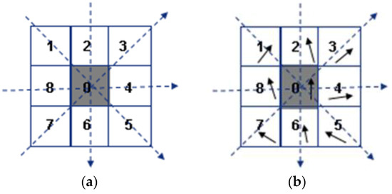
Figure 4.
The two modified LBP features. (a) M-LBP; (b) O-LBP.
The orientation threshold is selected based on the prior knowledge of face gradient distribution. There are different gradient variations along different directions in different regions. Most face landmarks are mainly gathered in the component region with strong and rich variations, like eyes, eyebrows, mouth. In contrast, there are very few landmarks distributed in smooth regions with weak and little variations, like the cheeks and forehead. Because the specific application in this paper is face alignment, the feature representation on the component regions should be highlighted. We hope to keep the above two regions with different gradient distributions as separate as possible. In the other words, the pixels labeled 1 and 0 after the binary process should be distributed in the two regions. A binary threshold based on gradient orientation is selected to maximize the distance between the two classes. We suppose that the pixel gradient orientations in the two regions satisfy the different gauss distributions. The mean and variance of gradient orientations in two regions are calculated. The junction position of two gauss curves is the threshold. The threshold cannot be set to 0 because the gradient orientations in the local neighborhood are not strictly equal due to illumination and noise, even in the smooth region with a similar texture. After multiple experiments, pi/8 was selected as the threshold, as it has the best classification effect and can tolerate local variations.
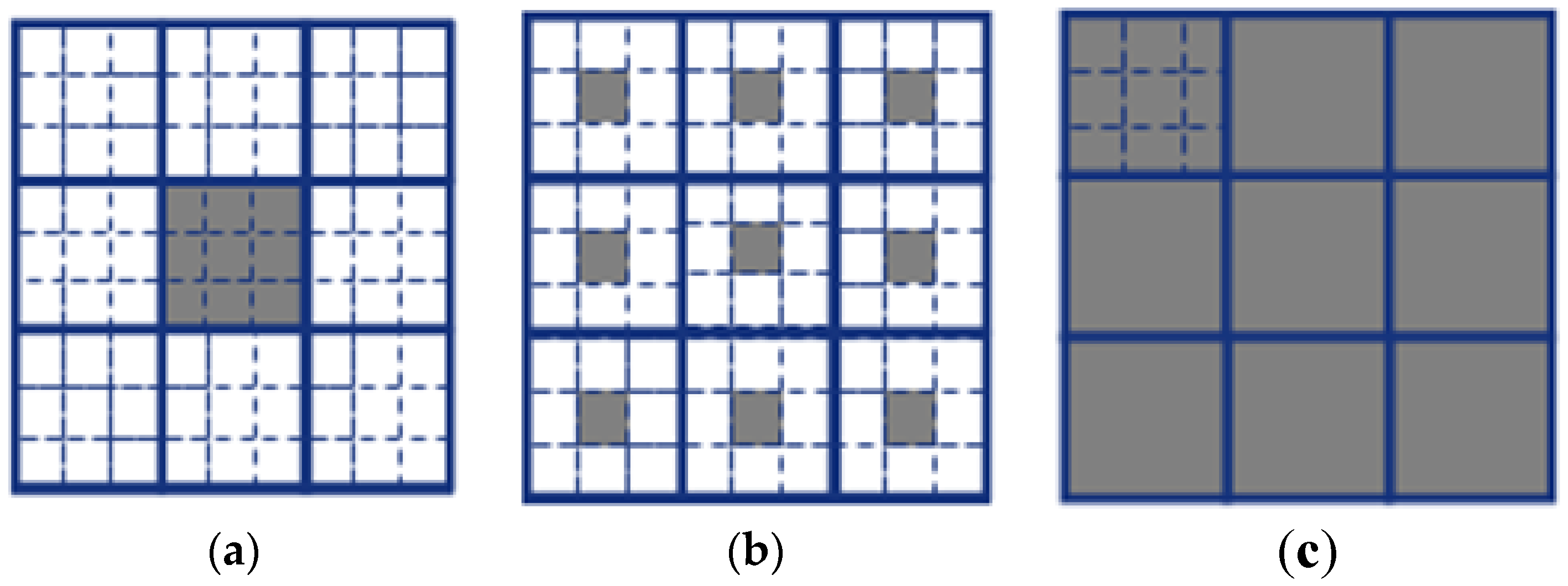
To combine multi-scale representation information, the three computing modes are further designed, including the original mode, the central mode and the average mode. The pixels in the different neighborhoods are selected for each mode. The adjacent pixels of the current pixel are selected for the original mode. The central pixels in the 3 × 3 adjacent blocks are selected for the central mode. The averages in the adjacent blocks are selected for the average mode. The grey regions in Figure 5 indicate the selected pixel set of different modes.
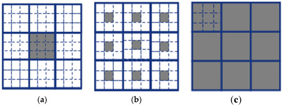
Figure 5.
The multi-scale feature extraction modes. (a) original mode; (b) central mode; (c) average mode.
The information along the four directions in M_LBP and O_LBP is respectively encoded into four binary codes. The two features are linearly concatenated into eight binary codes, which can produce 2^8 = 256 binary patterns, just like the original 8 neighbors LBP. The modified LBP features are extracted from each pixel and can be regarded as the pixel value of a grey image. Thus, the input image is encoded as the three LBP images which contain multi-scale representation information (as shown in Figure 6).
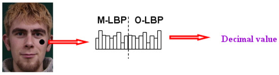
Figure 6.
The multi-mode LBP feature extraction and encoding.
3.2.2. Shape Parameters Regression Based on CNN
The shape PCA parameters can constrain common variations of whole face shape. Regressing shape parameters within lower dimension parametric space can decrease calculations, and tends to keep global constraint. Instead of the raw face image, according to the former description, the multi-mode LBP images are constructed and applied to regress the face shape parameters.
The traditional handcrafted features carefully designed based on expert knowledge only reflect limited aspects of a certain problem. Recently, deep learning algorithms have been widely applied in the face alignment field. However, deep learning requires a large number of training samples, which is not practical in some specific applications. Furthermore, the deep features do not always outperform the handcrafted features in all applications. Prior knowledge can be introduced and the more efficient and richer information can be obtained by combining the above features, which can achieve better alignment performance than single feature.
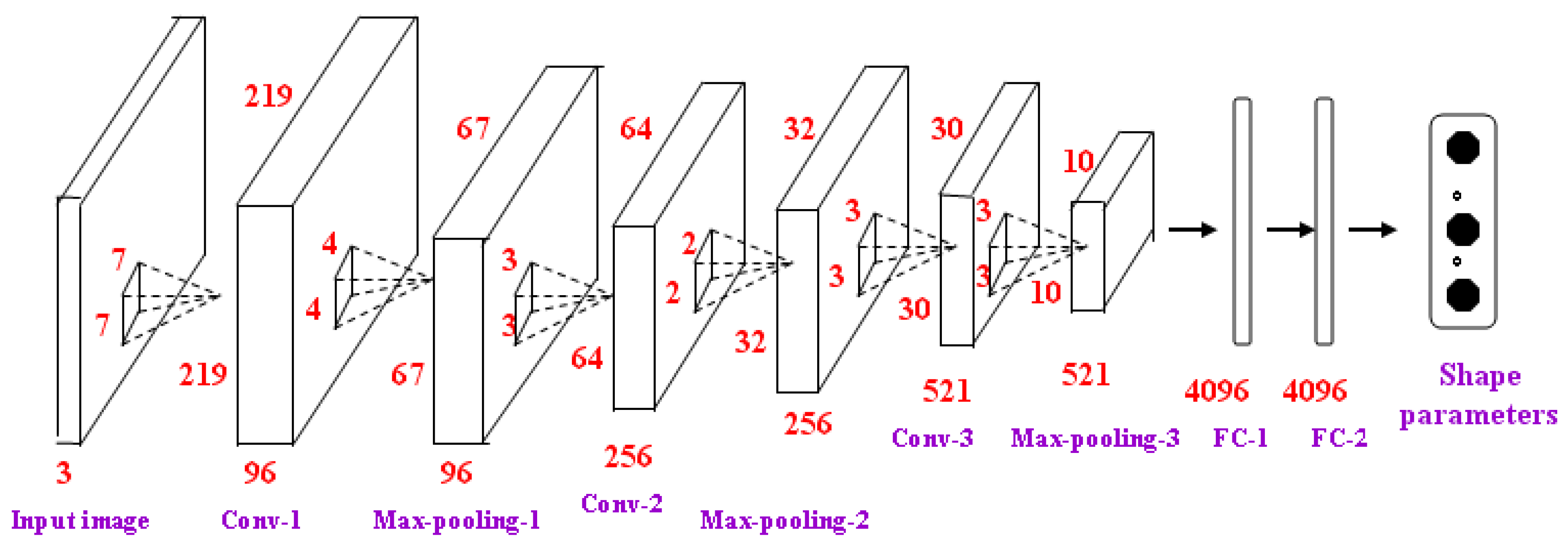
The global feature represented by multi-mode LBP images contains more distinguishable information than the original pixel-level image. So, a simpler network is enough to achieve the same performance as running a deeper network at pixel level. The architecture used here contains 3 convolutional layers, 3 max-pooling layers and 2 fully-connected layers (as shown in Figure 7). The number of neurons of the two FC layers is 4096. The three input multi-mode LBP images are normalized to 224 × 224.
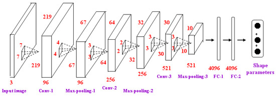
Figure 7.
The shape parameters regression based on the LBP images.
The model is trained by minimizing loss function with back-propagation. The SGD (stochastic gradient descent) method divides the training set into many mini-batches and updates the network parameters by a mini-batch data every time. Computation over a batch can be much more efficient due to the parallelism afforded by the modern computing platforms. Thus, model training with a large amount of data can successfully and quickly converge. The optimal parameters of the SGD method for training our CNN model are determined by experiments. The parameters are set as follows: Mini-Batch Size = 10, Initial Learning Rate = 0.001, Learning Rate Drop Factor = 0.1, Learning Rate Drop Period = 2 and Momentum = 0.9.
The distribution of the activations in the intermediate layers constantly changes during training, which slows down the training process in every training step. To reduce the internal covariate shift, the inputs of each layer within the network are normalized to obtain approximately the same distribution. Batch normalization has been the de facto standard in the industry since 2015 [56]. Many different popular deep leaning frameworks also adopt it as a standard setting. In this paper, batch normalization is performed after each convolution layer based on the mean and variance of the values in the current mini-batch (usually zero mean and unit variance). The procedures are as follows: (1) Calculate the mean and variance over a mini-batch. (2) Normalize the input by subtracting the batch mean and dividing by the batch standard deviation. (3) Scale and shift the normalized result to obtain the output. The normalized result is multiplied by a “standard deviation” parameter (gamma) and adds a “mean” parameter (beta). Batch normalization has the following advantages: (1) it increases the stability of a network and make learning process easier. (2) it speeds up convergence, uses higher learning rates and controls overfitting. (3) it reduces the sensitivity of the network to initial weights. The experiments show that batch normalization obtains 10 times or more improvement in the training speed.
Deeper networks can achieve better performance, but are difficult to train and converge. Accordingly, transfer learning based on ImageNet is performed on many tasks. Fine-tuning is necessary for pre-trained deeper networks, followed by own structure. Pre-training has been a general operation in the current computer vision field. However, He et al. [57] express a different opinion by experimentally comparing training from scratch with pretrained models. Training from scratch on target tasks requires more iterations to sufficiently converge. ImageNet pre-training can only speed up convergence on the target task and cannot improve the final accuracy. Finally, pre-training helps less if the target task is more sensitive to localization than classification. However, the application in this paper is face alignment, which is sensitive to landmark positions. Furthermore, many pretrained models are based on grayscale images and are mainly used for classification. This paper performs face alignment on the gradient LBP images and obtains better performance than with grey images. Accordingly, the current pretrained models are not suitable for our application.
Deeper networks require larger computations, and the corresponding performance do not increase infinitely as the number of layers increases. The number of network layers is determined after many experiments, in which the tradeoff between speed and effect is made. In this paper, there is no need to use a very large amount of computation for the global alignment because it is not the final result. The following process is performed for refinement. Because the handcrafted features applied in this paper contain a lot of prior knowledge, the network itself has a relatively simpler structure. In summary, the shallower networks are able to fulfill our task and have the corresponding advantages are fast convergence and easy training.
The ReLU function is selected as an activation function because it requires a shorter computation time compared to a non-linear activation function, and makes the model training easier. The 40% connections between the neurons in the two FC layers are disconnected by applying the dropout. The output of the FC2 layer is applied to regress the shape parameters. Thus, the whole face shape is updated and the global alignment is performed.
3.3. The Local Alignment Based on the Landmark Position Update
To represent the local information of a face, multiple features can be extracted on the component regions or the neighborhood around a landmark. To obtain more descriptive face representation, these features are extended by combining different scale information. The different multi scale features are widely applied in face alignment to achieve the better performance. Xin et al. [58] fuse the multi scale features to calculate the distance between two images. A significant improvement in performance over single scale histogram of oriented gradients (HOG) features is obtained. Cai et al. [59] effectively explore both deep-learned features and the weighted HOG feature. The fused features are fed to a softmax classifier for pedestrian gender recognition. Supervised Descent Method (SDM) learns a sequence of descent directions that minimize the difference between the estimated shape and the ground truth in HOG feature space, and utilize them to predict shape increments iteratively [23]. Liu et al. [60] modify SDM in three respects, i.e., multi-scale HOG features, global to local constraints and rigid regularization. Song et al. [61] combines local/global shapes and local textures to construct the eye state model. Multi-scale Histograms of Principal Oriented Gradients are proposed.
In this paper, the multi-mode HOG features around each landmark are extracted and encoded as scalar values. The redundant and more representative information in the local region is applied as the input to a trained random regression forest. Each landmark position is independently regressed and updated, at which time the shape details are further precisely adjusted. Random regression forests can be efficiently performed on parallel architectures, which results in fast calculation times.
3.3.1. Multi-Mode Local Feature Representation
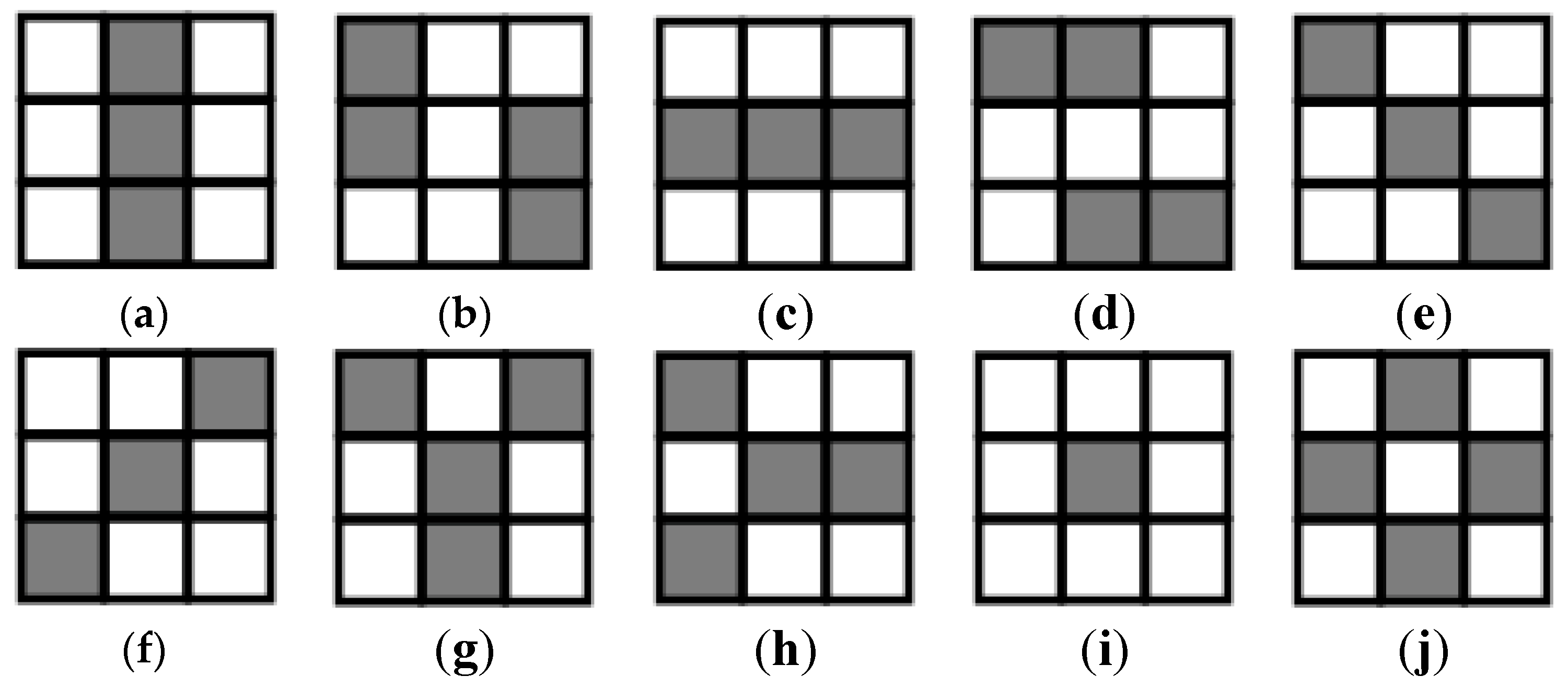
HOG is powerful appearance representation tool, but it is inefficient at discovering intrinsic and essential characteristics of face variation by single scale analysis. In this paper, the multi-scale and multi-direction local information is encoded as multi-mode features so as to extend the representation power. The multiple square patches contain 3n × 3n blocks around a landmark are selected to extract the features in variable scales along different directions. The six categories and ten kinds of features are extracted, i.e., Horizontal Mode, Vertical Mode, Ascending Mode, Descending Mode, T Mode and Center Mode (as shown in Figure 8). The size of a patch reflects the influence range of local features and is chosen according to face size and image resolution.

Figure 8.
The different feature extraction modes. (a)Vertical Mode1; (b) Vertical Mode2; (c) Horizontal Mode1; (d) Horizontal Mode2; (e) Descending Mode; (f) Ascending Mode; (g) T Mode1; (h) T Mode2; (i) Center Mode1; (j) Center Mode2.
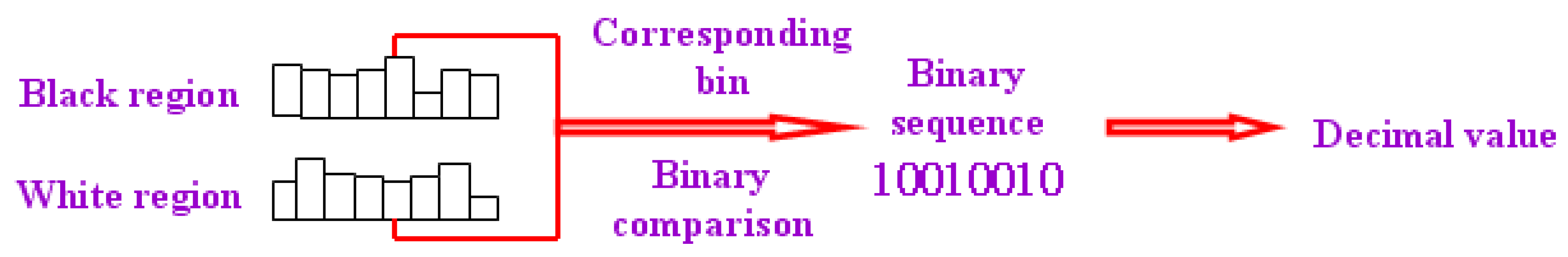
Each pixel in a black (or white) region casts a weighted vote in an orientation-based histogram with its magnitude as the weight. The different feature modes may cover the overlapping regions, but represent different local texture information. The HOG features of black and white region in each mode are respectively calculated, and the corresponding bins are compared as follows:
where and indicate the bins of black and white region histograms, indicate the index of component. Then a binary sequence is obtained and 8-bit binary values can be converted to a decimal number by , within the range of 0~255.
The black-white distribution in each feature mode region is represented as a number, and the multi-mode redundant information can be concentrated into a series of scalars (as shown in Figure 9). The gradient calculation over the original image is performed in the process of encoding multi-mode LBP images. Here, all HOG features are obtained by reorganization and count on the gradient image, according to different feature modes.
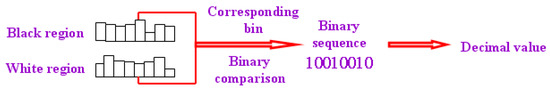
Figure 9.
The local feature extraction and encoding.
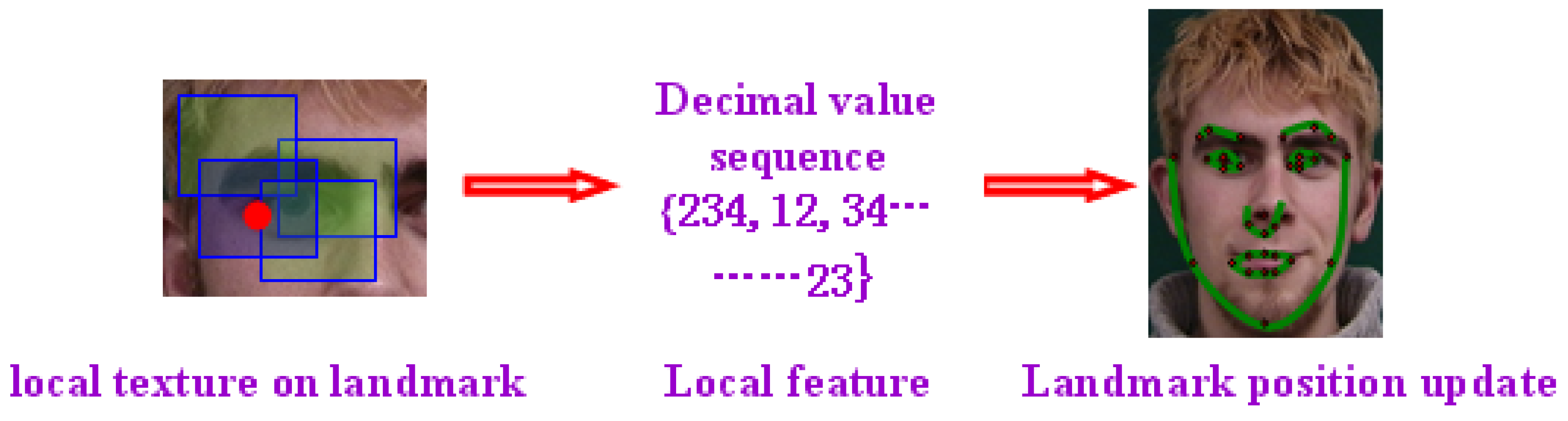
3.3.2. Landmark Position Update Based on Random Regression Forests
The shape details are carefully adjusted by regressing and updating each landmark position based on the local feature respectively. Several patches are obtained by random sampling centered around a landmark on images. The red point indicates the ground-truth of right outer eye corner and the other green patches indicate the random sampling regions (as shown in Figure 10).

Figure 10.
The landmark position update based on local feature regression.
The training samples contain a set of paired data, where indicates the neighboring patch around a landmark and indicates the corresponding displacement. According to the former description, the multiple kinds of multi-mode HOG features are extracted and encoded at random sampling patches around a landmark to form a large number of redundant local features.
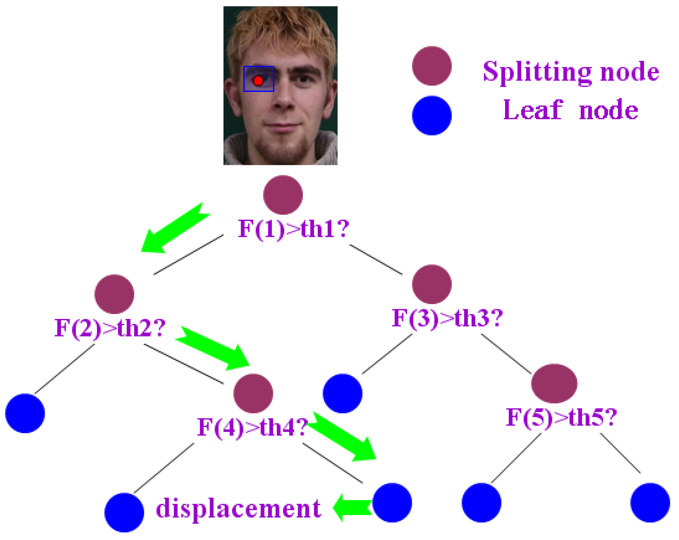
Random forests have been used successfully in many classification and regression problems. They represent a simple and efficient algorithm with few free parameters, and have shown resistance to overfitting. Random forests are constructed by building a set of n binary trees on bootstrap samples from the training dataset. By randomly selecting the splitting feature and the threshold from the large feature set, the best binary criterion is found to split samples. According to a standard procedure, starting from the root node, the non-leaf nodes are spitted by the binary test which is randomly selected until the sample set is divided into left branch and the right branch .
By minimizing the least square error (LSE) of sample data
the best binary split of each node is obtained. Here, indicates the output displacement of the kth sample, and respectively indicate the number of samples from left and right branch, and respectively indicate the mean output displacement of samples from the corresponding branches.
The tree is constructed in a recursive way and will stop growing when it reaches the given depth, or there are too few samples left or else the variance of the node is smaller than one threshold. Each leaf node stores the average displacement of all sample output. The predicted result of the whole forests is obtained by averaging the predicted results of all trees (as shown in Figure 11). The current patch is fed into the trained random forests to update the displacement vectors during the test. Because each tree of random forests is uncorrelated and every landmark is independently updated, both the training and testing stages can be efficiently performed on parallel architectures.

Figure 11.
The landmark position update based on the random regression forests.
3.4. Weighted Integration of the Global and Local Alignment
The alignment on the contours of mouth and chin converge to local optima due to partial occlusions, as shown in Figure 12a. The error on the chin contour is related to the attraction of the similar skin background, while the error in the eyebrow region is caused by illumination variation, as shown in Figure 12c. The two alignment results from global and local are integrated according to the weights.
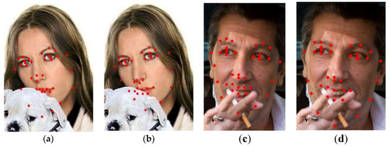
Figure 12.
Improvement for the images under the different conditions. (a) local optima on the contours of chin due to partial occlusions; (b) the improvement for the influence of occlusion; (c) misalignment in eyebrow region caused by illumination variation; (d) improvement for the influence of illumination.
Here, all landmarks are classified into different face components, including eyebrows, eyes, nose, mouth, chin, cheeks, and contours. The different alignment shapes within each component are weighted as , where indicates the index of certain component, , and respectively indicate the weighted, local and global shape within the current component, indicates the corresponding weight.
The weights are determined by minimizing the residual between the weighted shape and the corresponding ground-truth on all training images, i.e.,
where indicates the index of train image. The weight in the above formula can be calculated by least square method. The weights within each component are obtained one by one. Then, the alignment shapes from global and local are weighted as the final result. As shown in Figure 12b,d, the final face shape achieves the global optimum and local refinement jointly.
4. Experimental Results and Analysis
In order to evaluate the performance of our algorithm, comparative experiments with several popular algorithms are performed on the public databases. The ground-truth of landmarks served as a benchmark, and the qualitative analysis and quantitative comparison is presented.
4.1. Experimental Setup
To analyze the performance on different image data, the following four databases are used.
(1) The BioID Face Database consists of 1521 gray level images with a resolution of 384 × 286 pixels. Each of the 23 different tested persons shows the frontal view of the face. All of images are extracted from face video with different backgrounds.
(2) The IMM Face Database comprises of 240 still images with resolutions of 640 × 480 pixels. Each of the 40 individuals presents variations of head pose and expression. The background variation is not significant and the illumination in the whole image is not even.
These two databases are conducted under controlled conditions and with a simple background. The former is more useful to test the robustness of the algorithm to illumination variations and expressions, whereas the latter is more suitable to see the influence of image resolution in face alignment. In this paper, the images from these two databases are divided into two parts: 1/4 images comprised the training set and 3/4 comprised the test set.
(3) The LFPW Face Database consists of 1035 face images, 811 images comprised the training set and 224 comprised the test set.
(4) The HELEN Face Database consists of 2330 face images with a higher resolution, 2000 images comprised the training set and 330 comprised the test set.
The images of these two databases are from the internet, with no control and great variations in illumination, occlusion and expressions.
It is easy to encounter overfitting problems with a small amount of training data for the CNN networks used in this paper. Therefore, a widely used data augmentation technique is performed to obtain more training images. The additional images are artificially created from the existing images by using image translation and cropping. Finally the training image volume is significantly increased.
As a preparation task, the landmark positions in all sample images are obtained, and a set of landmark coordinates on each image form a face shape vector. The following quantitative evaluation indicators were used to measure the alignment accuracy on the test samples.
(1) Normalized error: The error distribution of all images can be obtained from mean and max error of all landmarks in each image. To remove the influence of the image size, the normalized error is defined as , where indicates the index of landmark, and respectively indicates landmark position automatically aligned and manually labeled, indicates the distance between eyes in front face image or the size of bounding box.
(2) Success rate: In the alignment process, if the algorithms cannot converge when the iterations reach the max or the error between the convergence results and the labeled results is greater than a certain threshold (like 5%), it can be concluded that the alignment on this landmark failed. The proportion of the landmarks which were successfully aligned reflects the algorithm performance.
4.2. The Performance Analysis
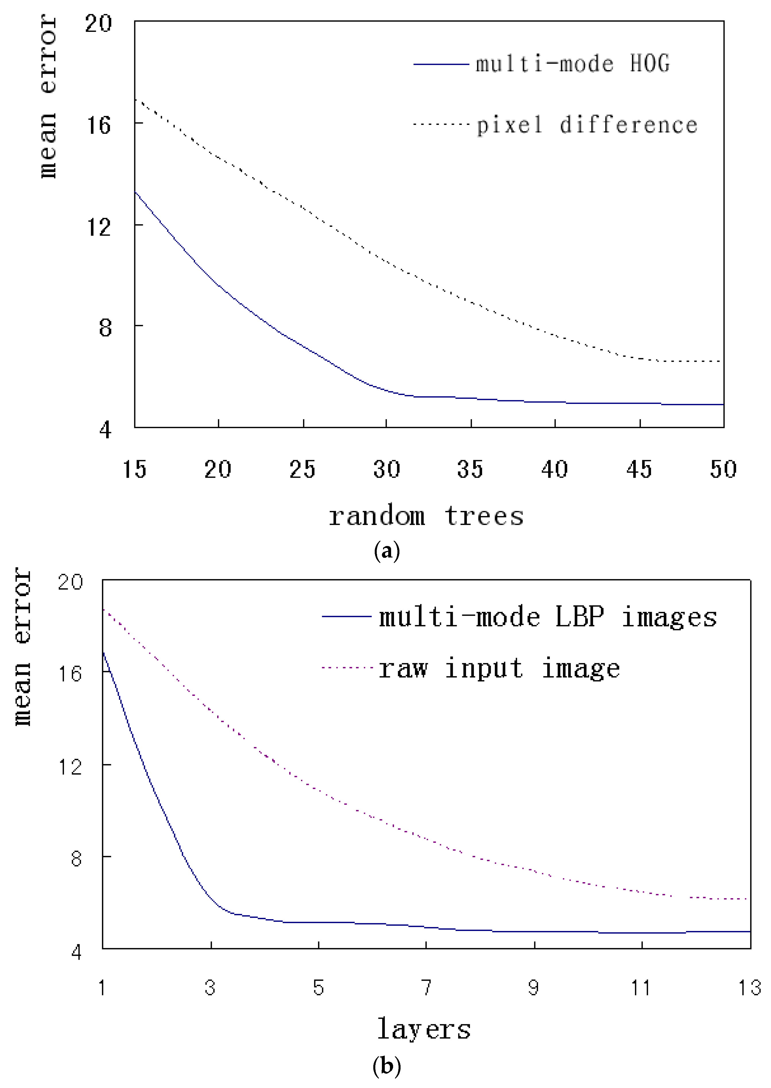
In this paper, the proposed multi-mode features were extracted and encoded for a whole face or a local region. The algorithm performance based on the different features was compared. The two features were respectively applied for the local alignment, including the pixel difference feature and the multi-mode HOG feature. The global alignment was performed on the raw input image and the multi-mode LBP images. The corresponding results of the above methods on HELEN database were quantitatively compared. Figure 13a,b respectively indicates local alignment and global alignment.
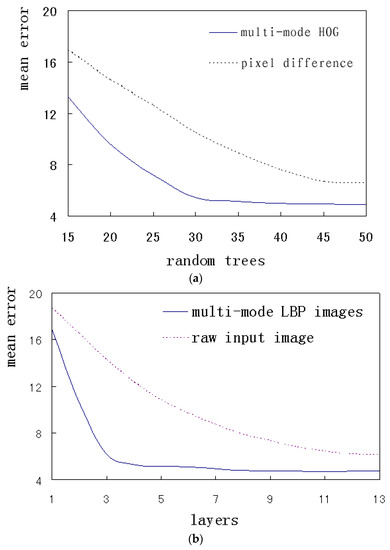
Figure 13.
The error comparisons of the different features. (a) The error variation with the number of random trees; (b) The error variation with the number of CNN layers.
Figure 13a shows how the average errors change when the number of random trees increases, where multi-mode HOG features and pixel difference features are respectively applied. It can be seen that the errors decreases gradually as the number of random trees increases. The error of the multi-mode HOG features rapidly decreases and reaches saturation at 30 trees, while the pixel difference features achieve the same situation at 45 trees. The above results show that the multi-mode HOG features are more descriptive and distinguishable. Consequently, this method can adopt simpler architectures and achieve better performance and faster convergence. The error will not decrease indefinitely, and tends to saturation after the trees reach a certain number. To avoid over-fitting specific data, the trade off between the complexity and performance should be investigated to choose the appropriate calculation size. The parameters of the random forests for the local alignment are set to the optimal situation, the number of trees is 30 and the depth is 5.
Figure 13b shows how the average errors change when the number of CNN layers increases, where multi-mode LBP images and raw input images are respectively applied. It can be seen that the errors decrease gradually as the number of CNN layers increases. The error of the multi-mode LBP images reaches the saturation at 3 layers, while the raw input images achieve the same situation at 12 layers. The above results show that the multi-mode LBP images can obtain more efficient and richer information by introducing prior knowledge. Consequently, this method can adopt simpler architectures. CNN networks for the global alignment adopt 3 layers.
The errors in Figure 13a are lower than those in Figure 13b, which shows that the performance of local method is better than that of the global method. The global method cannot get a better representation with local details.
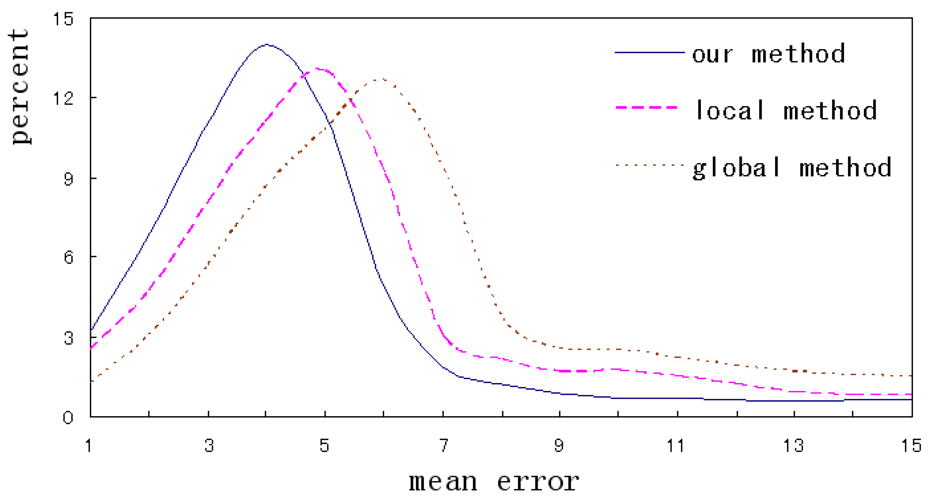
This paper evaluates the alignment accuracy by the error distribution of landmarks in one image. Figure 14 intuitively shows the distribution curves of the different methods on LFPW database. It can be seen that the errors of our method mainly distribute in the range of 3~5, and the range is 4~6 and 5~7 for the local and global method respectively. From the proportion of errors over 8, the global method is the highest and our method is the lowest. The total error distribution indicates that the accuracy of our method is higher than that of the single method. Therefore, integrating the outputs of the different alignments helps to accurately describe the details and contours of a face.
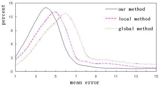
Figure 14.
The error distribution of the different methods.
Shape initialization can be achieved by directly averaging all sample shapes or by applying 2D affine transformation on the mean shape. Our method performs a series of CNNs on the patches around the anchor landmarks to regress affine transformation parameters. The performance of the above methods is evaluated and compared by the mean error of the initial shapes. It can be seen from Figure 15 that our method has fewer errors than other methods based on mean shape. The variation tendency on several databases keeps accordance. Our method using the IMM database has the fewest errors, and the mean shape on HELEN database has the most. In general, the images on HELEN and LFPW have larger pose variations, which leads to a higher number of initialization errors than those on BioID and IMM.
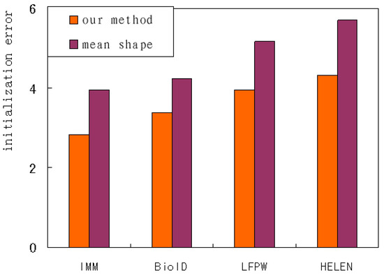
Figure 15.
The initialization error of the different methods.
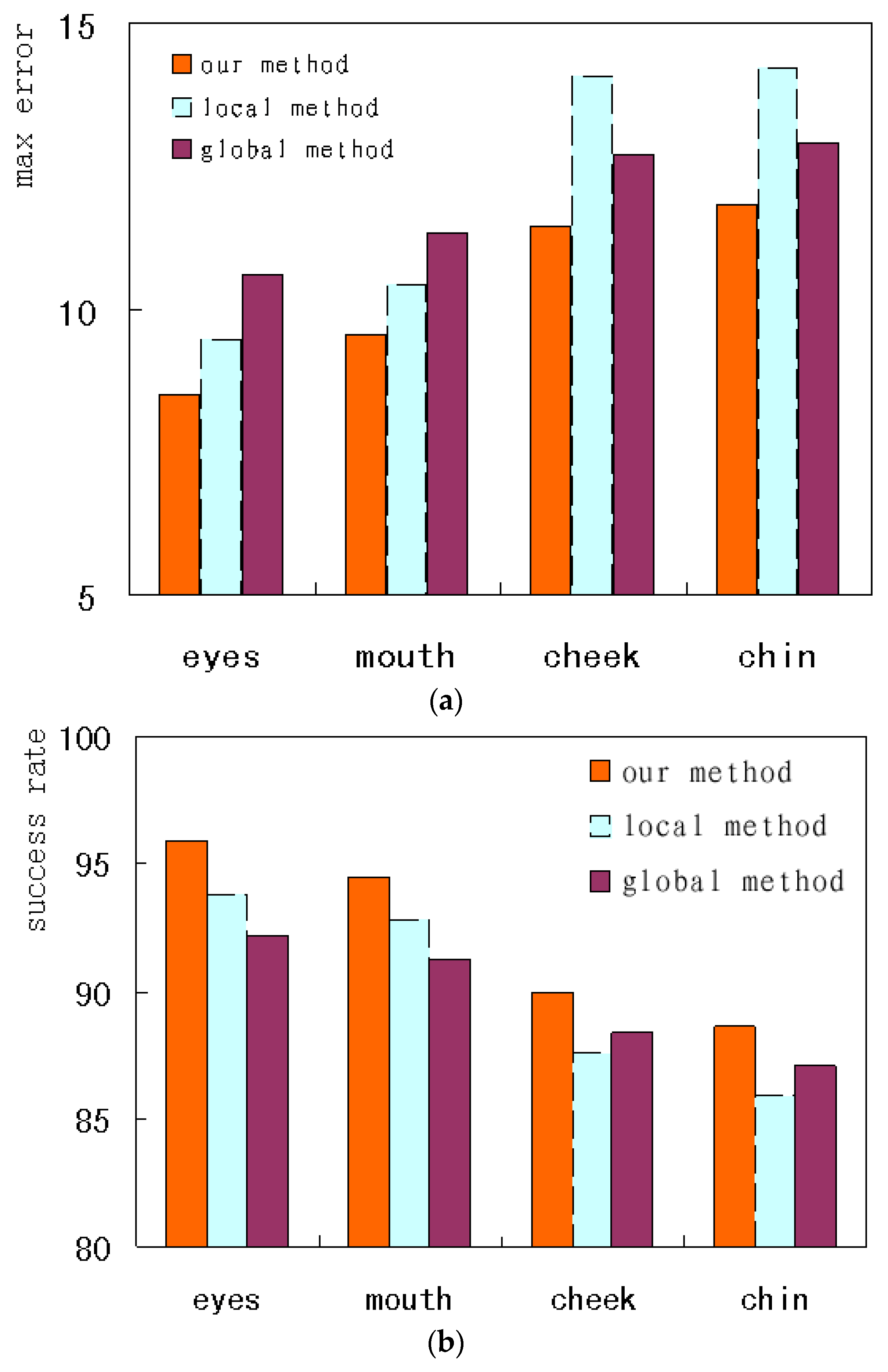
To compare the performance on the different landmarks, this paper investigates the accuracy of face alignment on the internal regions and the external contour. The comparisons on the HELEN database are shown. Figure 16a,b respectively indicates the max error and the success rate of the alignment on the different landmarks. From Figure 16a, it can be seen that our method for the eyes has the lowest max error, i.e., less than 8.5. The local method on the chin has the largest max error, higher than 12. On the eyes and mouth, the local method has a lower max error than the global method. But on the cheek and chin, the global method has a lower max error. From Figure 16b, it can be seen that our method on the eyes has the highest success rate, i.e., higher than 95%. The local method on the chin has the lowest success rate, less than 86%. On the eyes and mouth, the local method has a higher success rate than the global method. But on the cheeks and chin, the global method has a higher success rate. The above results show that the local method tends to converge to the local optimum in those regions what have few texture variations; additionally, the global method can reach the global optimum on the contours. The performance can be improved by combining different methods applied to different face regions. Accordingly, our method on the eyes has the best performance.
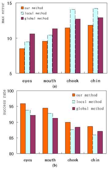
Figure 16.
The performance comparison of the different regions on LFPW database. (a) max error; (b) success rate.
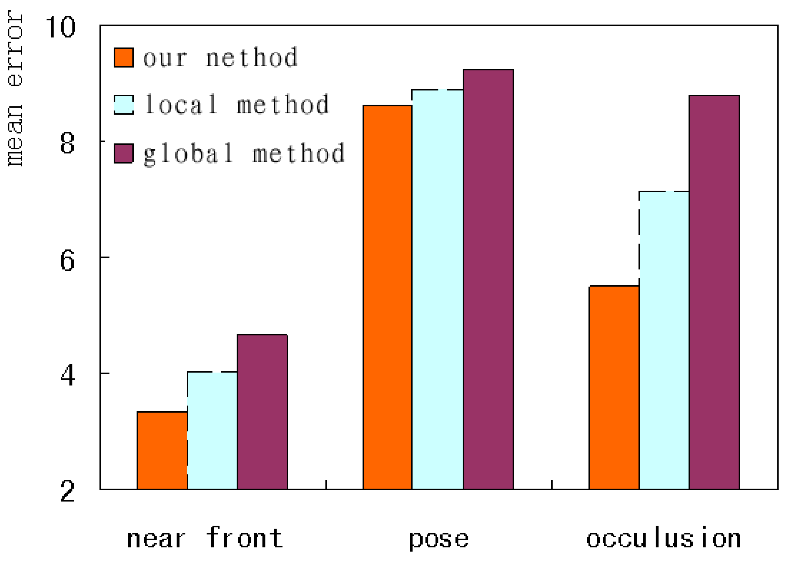
To further analyze the performance under different image conditions, this paper selected three kinds of test images, i.e., near-front, pose and occlusion, to form the difficult test set, and investigates the corresponding mean errors. As shown in Figure 17, our method has the fewest errors, and the global method has the most. The variation tendency under the three kinds of conditions remains in accordance. Our method improves performance by globally constraining the shape and carefully adjusting the local contour simultaneously.
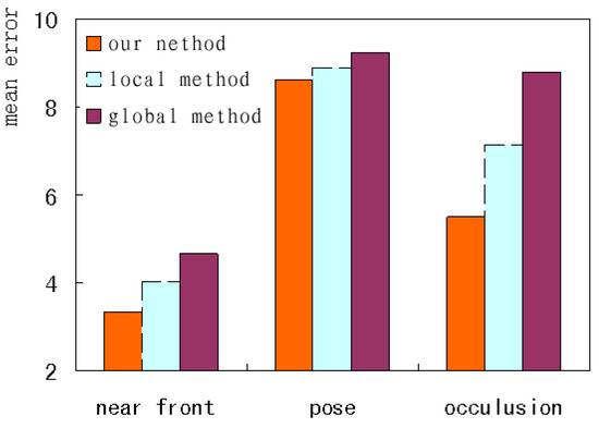
Figure 17.
The error comparison under the different conditions.
Complete texture information and reasonable shape constraint can be obtained when a face is close to the front. The near-front faces have the best performance for the three kinds of images. Our method applied to these images has the lowest mean error, less than 3.5. Partial occlusion can cause the loss of local information and the wrong convergence location based on the wrong texture. Faces under local occlusion increase the alignment difficulty and have the worst performance among the three kinds of images. Our method has the lowest mean error, less than 6. When large pose variations occur, severe self-occlusion will change the face structure because of the lack of depth information. Those landmarks on contour edges tend to be influenced by pose variation. The faces with pose have the worst performance among the three kinds of images. The error of the global alignment reaches 9.2, and the error of our method is reduced by less than 0.5. This shows that it’s not enough to combine global and local information when the face has too large a pose. Three-dimensional models or multi model sets with different poses should be introduced to represent the depth information or non-linear variation, which helps face alignment across large poses.
4.3. Comparison Experiment
To quantitatively evaluate the performance of our algorithm, the following four popular algorithms are chosen for comparison.
- (1)
- Explicit Shape Regression (ESR) performs cascade shape regression for face alignment by minimizing regression error [26].
- (2)
- Supervised descent method (SDM) minimizes the Non-linear least squares objective using the learned a sequence of descent directions [23].
- (3)
- Cascade gaussian regression (CGR) builds gaussian process trees for landmark position regression based on cascade stage-wise manner [21].
- (4)
- Deep neural network (DNN) extracts local features for optimization and the resulting deep regressor gradually and evenly approaches the true landmarks stage by stage [42].
These methods have been widely used in recent years and have achieved the best performance on larger databases. They are excellent in accuracy and computing speed, especially for alignment under real environments.
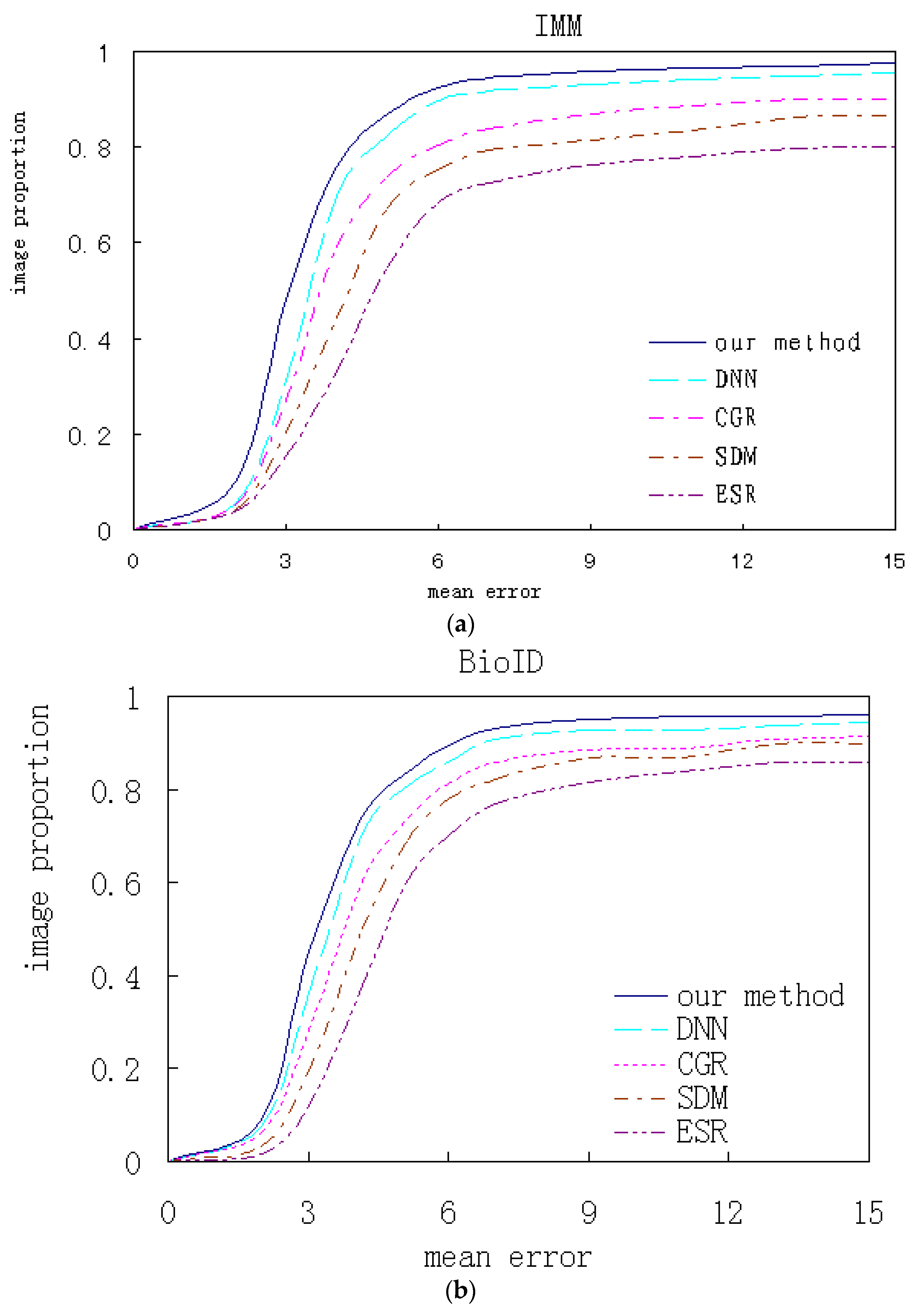
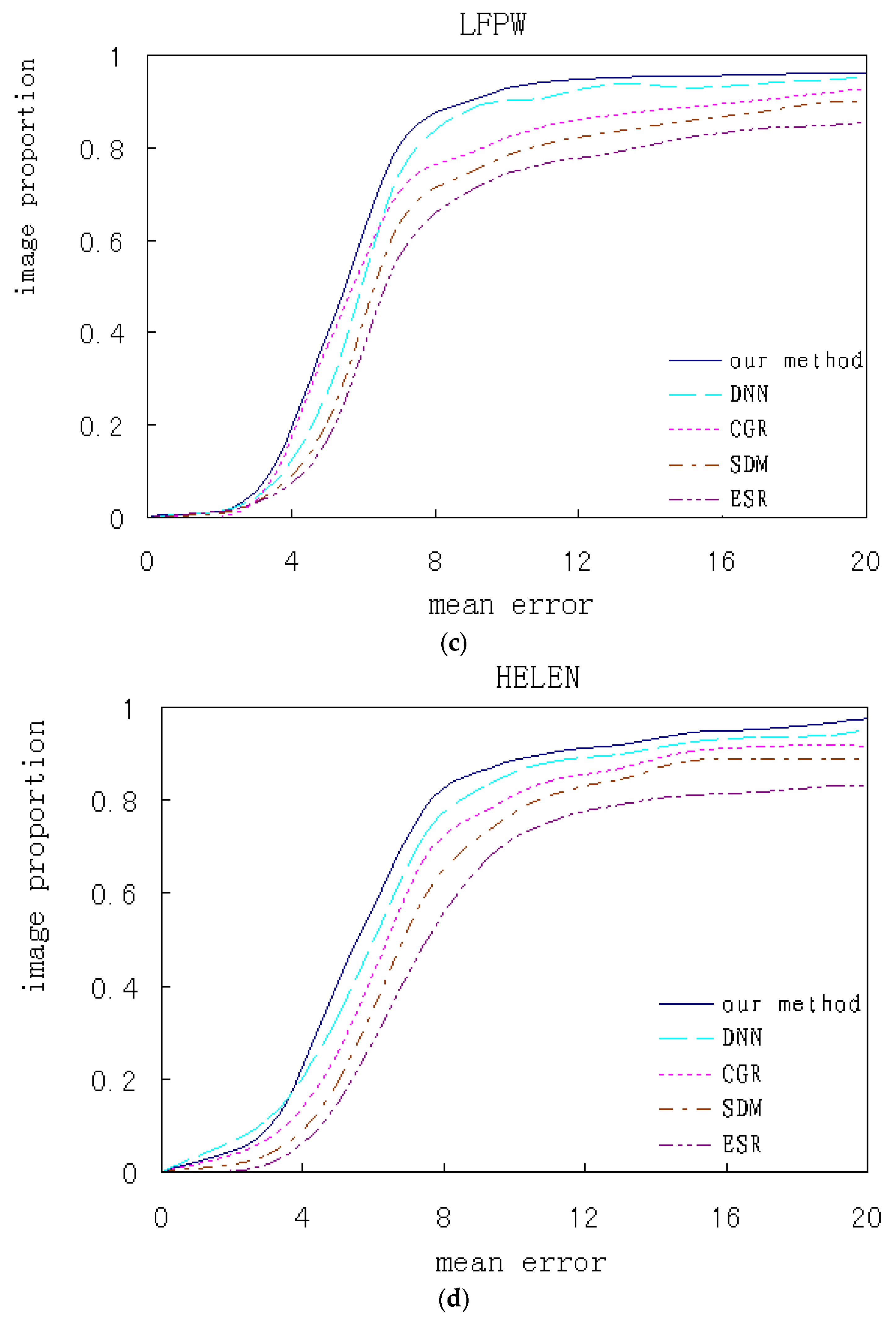
Our algorithm and the contrastive ones are respectively trained and test experiments are performed on several databases. The qualitative analysis and quantitative comparison based on the corresponding experimental results are shown. Figure 18 shows the cumulated error curves of different algorithms on different databases, where the x-coordinate indicates mean alignment error and the y-coordinate indicates test image proportion.
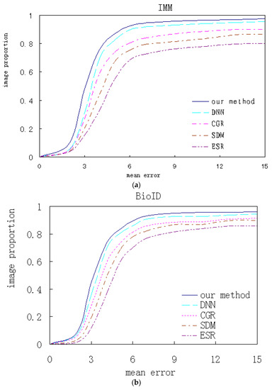
Figure 18.
The algorithms performance comparison on the different databases. (a) IMM; (b) BioID; (c) LFPW; (d) HELEN.
All faces from the IMM database are front. Some faces from BioID database have a slight pose and all landmarks are visible. On these two databases, our algorithm respectively has 81.5% and 78.1% samples with the average error of less than 4, which is higher than the contrasted ones. Most faces from the LFPW database are close to the front, while many images with higher resolution from HELEN database are non-front and have relatively low accuracy. On these two databases, our algorithm respectively has 83.9% and 81.1% samples with average error of less than 8 respectively. Although the performance is still relatively better, the improvement of our method is limited for faces over a certain angle.
In contrastive methods, our method has the best performance and ESR has the worst. The variation tendency on the four databases keeps accordance. Compared with deep learning methods, traditional methods based on the local features and global regression, including ESR, SDM and CGR, have lower accuracies because the simple local features and rough linear regression cannot handle the non-linear alignment problem. Our method introduces prior knowledge into the CNN networks and integrates global and local alignment, which can achieve better performance compared to a single CNN.
The above comparitive results indicate that the single global or local method is insufficient to describe complicated face texture variations and is very sensitive to tremendous variations of occlusion and illumination, both of which lead to worse performance. The multi-mode features are more descriptive than single scale features, and the combination of the two alignments has huge advantages, which helps to handle the nonlinear variation caused by illumination and occlusion.
The hardware configuration in this paper is as follows: A 3.33 GHz i7 CPU, 16 GB RAM, a GeForce GTX 1070 graphics card. All algorithms in this paper are partially optimized. Table 1 compares the corresponding computation efficiency on different databases by the mean time of one image. It can be seen that more complex methods take longer, and the tendency on different databases keeps accordance.

Table 1.
The efficiency comparison of different methods on different databases (ms).
Compared with the former two databases, LFPW and HELEN databases have more non-front faces under more difficult conditions, which partially increases the computational complexity. The maximum demands of our method are due to the multi-mode feature extraction and encoding. Moreover, the two alignments are performed and integrated. Naturally, the calculation consumption is greater than the other algorithms. But the features and methods we proposed are more descriptive and more effective, which can achieve better performance.
Compared with contrastive ones, the calculation speed of our method on current popular computers has no significant reduction. The calculation efficiency almost reaches real-time. Therefore, as a whole, our method truly helps to boost the performance while the computational complexity increases only a little.
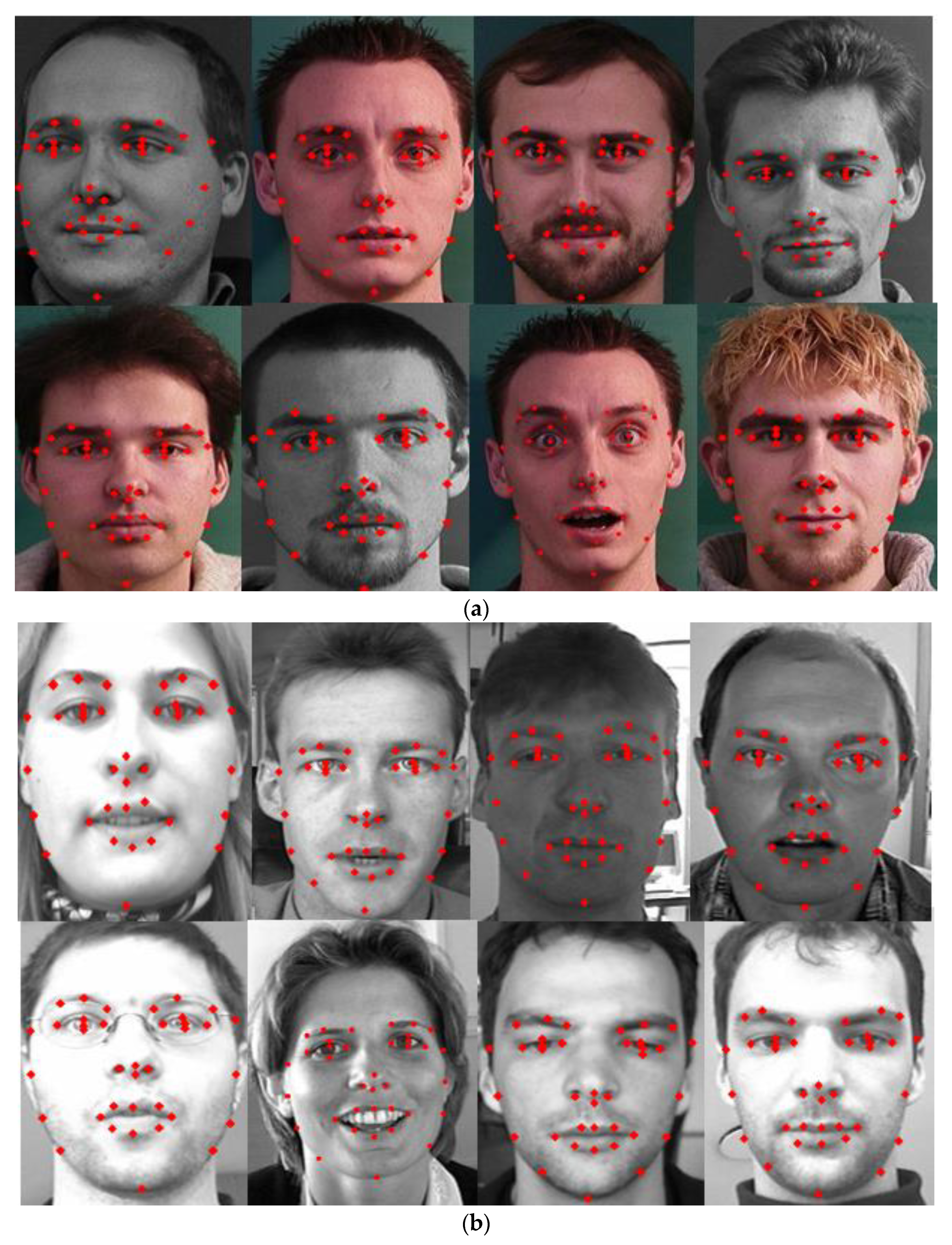
Figure 19 exhibits some experimental results on some images selected from the four databases based on our method. It can be seen that the performance is excellent on each database. Because our method learns the a priori knowledge of face shape by global featurea and is relatively robust to background and local noise, we can obtain better alignment effects under different illuminations, expressions and with partial occlusion.
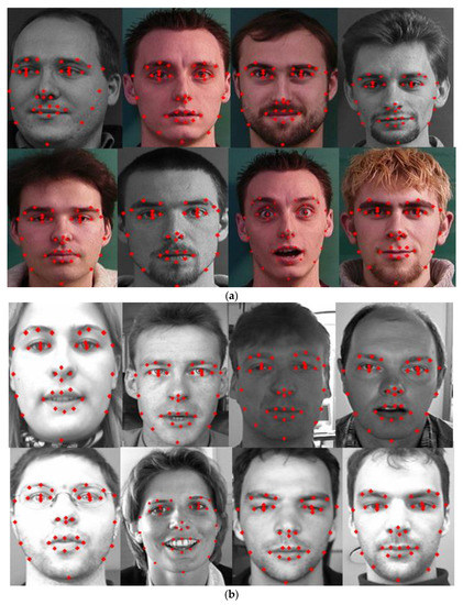
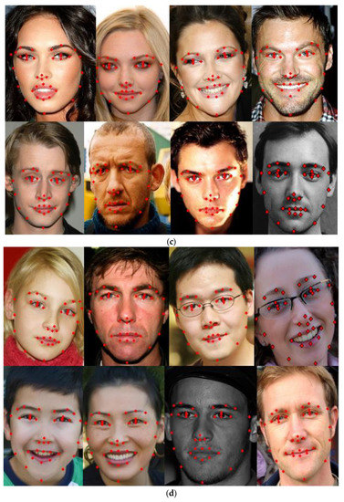
Figure 19.
Some alignment results on the samples from the different databases. (a) IMM; (b) BioID; (c) LFPW; (d) HELEN.
5. Conclusions and Future Work
This paper jointly considers appearance representation and alignment strategy. The global match of the whole face and the local refined correction of given regions are integrated and embedded into a multi-layer progressive face alignment framework. The redundant multi-mode information from a given region or a whole face is encoded as a local and global feature. The shape initialization and face shape update is performed by applying different alignment strategies based on the multiple representation features. By weighted integration and a coarse-to-fine alignment strategy, our method can deal not only with the influences due to illumination variation and local noise, but can also compensate for partial occlusion by global constraints. The final shape achieves the global optimum and the local refinement jointly. Our experiments on public databases indicate that the method improves the performance while the corresponding complexity increases only a little.
In future, a straightforward continuation of this work would be to keep optimizing our system to satisfy the demand for automatic and real-time applications. Furthermore, we will enhance the alignment performance on the images under the large expressions and poses by extending our method to multi-state face representation space or introducing the 3D face model.
Author Contributions
N.G. and X.W. designed the different experiments; X.W. set up the corresponding experiment environment and performed the experiments; X.W. analyzed the experimental data; N.G. and X.W. wrote the paper. X.W. helped to modify the early version of the paper. X.W. helped to modify the later version.
Funding
This research was funded by Natural Science Foundation of China (Nos. 61672124, 61370145 and 61173183) and the Password Theory Project of the 13th Five-Year Plan National Cryptography Development Fund (No. MMJJ20170203).
Conflicts of Interest
The authors declare no conflict of interest.
References
- Tzimiropoulos, G.; Pantic, M. Optimization Problems for Fast AAM Fitting in-the-Wild. In Proceedings of the IEEE International Conference on Computer Vision, Sydney, Australia, 1–8 December 2013; pp. 593–600. [Google Scholar]
- Navarathna, R.; Sridharan, S.; Lucey, S. Fourier Active Appearance Models. In Proceedings of the IEEE International Conference on Computer Vision, Barcelona, Spain, 6–13 November 2011; pp. 1919–1926. [Google Scholar]
- Sun, Y.; Wang, X.; Tang, X. Deep Convolutional Network Cascade for Facial Point Detection. In Proceedings of the IEEE International Conference on Computer Vision and Pattern Recognition, Portland, OR, USA, 25–27 June 2013; pp. 3476–3483. [Google Scholar]
- Trigeorgis, G.; Snape, P.; Nicolaou, M.A. Mnemonic Descent Method: A Recurrent Process Applied for End-to-End Face Alignment. In Proceedings of the IEEE International Conference on computer vision and pattern recognition, Las Vegas, NV, USA, 27–30 June 2016; pp. 4177–4187. [Google Scholar]
- Zhang, J.; Shan, S.; Kan, M. Coarse-to-Fine Auto-Encoder Networks (CFAN) for Real-Time Face Alignment. In Proceedings of the European Conference on Computer Vision, Zurich, Switzerland, 6–12 September 2014; pp. 1–16. [Google Scholar]
- Sun, P.; Min, J.K.; Xiong, G. Globally Tuned Cascade Pose Regression via Back Propagation with Application in 2D Face Pose Estimation and Heart Segmentation in 3D CT Images. In Proceedings of the IEEE International Conference on Computer Vision and Pattern Recognition, Boston, MA, USA, 8–10 June 2015. [Google Scholar]
- Wu, Y.; Ji, Q. Discriminative Deep Face Shape Model for Facial Point Detection. Int. J. Comput. Vis. 2015, 113, 37–53. [Google Scholar] [CrossRef]
- Gary, S.; Ahmed, B.; Richard, J. Integrated Deep Model for Face Detection and Landmark Localization From “In The Wild” Images. IEEE Access 2018, 6, 74442–74452. Available online: http://nrl.northumbria.ac.uk/36374/ (accessed on 3 January 2019).
- Rajeev, R.; Vishal, P.; Rama, C. HyperFace: A Deep Multi-Task Learning Framework for Face Detection, Landmark Localization, Pose Estimation, and Gender Recognition. IEEE Trans. Pattern Anal. 2019, 41, 362–371. [Google Scholar]
- Zhang, K.; Zhang, Z.; Li, Z. Joint Face Detection and Alignment Using Multitask Cascaded Convolutional Networks. IEEE Signal Proc. Lett. 2016, 23, 1499–1503. [Google Scholar] [CrossRef]
- Zhu, S.; Li, C.; Loy, C.C. Unconstrained Face Alignment via Cascaded Compositional Learning. In Proceedings of the IEEE International Conference on Computer Vision and Pattern Recognition, Las Vegas, NV, USA, 27–30 June 2016; pp. 3409–3417. [Google Scholar]
- Kumar, A.; Chellappa, R. Disentangling 3D Pose in a Dendritic CNN for Unconstrained 2D Face Alignment. In Proceedings of the IEEE International Conference on Computer Vision and Pattern Recognition, Salt Lake City, UT, USA, 18–22 June 2018; pp. 430–439. [Google Scholar]
- Feng, Y.; Wu, F.; Shao, X. Joint 3D Face Reconstruction and Dense Alignment with Position Map Regression Network. In Proceedings of the European Conference on Computer Vision, Munich, Germany, 8–14 September 2018; pp. 557–574. [Google Scholar]
- Jourabloo, A.; Liu, X. Pose-Invariant Face Alignment via CNN-Based Dense 3D Model Fitting. Int. J. Comput. Vis. 2017, 124, 187–203. [Google Scholar] [CrossRef]
- Fan, L.; Tao, X.; Tong, S. Kernel PCA and Nonlinear ASM. In Proceedings of the IEEE International Conference on Control Systems, GangWon, Korea, 17–20 October 2018; pp. 287–293. [Google Scholar]
- Zhao, X.; Kim, T.; Luo, W. Unified Face Analysis by Iterative Multi-output Random Forests. In Proceedings of the IEEE International Conference on Computer Vision and Pattern Recognition, Columbus, OH, USA, 23–28 June 2014; pp. 1765–1772. [Google Scholar]
- Asthana, A.; Zafeiriou, S.; Cheng, S. Robust Discriminative Response Map Fitting with Constrained Local Models. In Proceedings of the IEEE International Conference on Computer Vision and Pattern Recognition, Portland, OR, USA, 25–27 June 2013; pp. 3444–3451. [Google Scholar]
- Zadeh, A.; Baltrusaitis, T.; Morency, L. Deep Constrained Local Models for Facial Landmark Detection. In Proceedings of the IEEE International Conference on Computer Vision and Pattern Recognition, Las Vegas, NV, USA, 27–30 June 2016. [Google Scholar]
- Saragih, J.M.; Lucey, S.; Cohn, J.F. Deformable Model Fitting by Regularized Landmark Mean-Shift. Int. J. Comput. Vis. 2011, 91, 200–215. [Google Scholar] [CrossRef]
- Tzimiropoulos, G.; Pantic, M. Gauss-Newton Deformable Part Models for Face Alignment In-the-Wild. In Proceedings of the IEEE International Conference on Computer Vision and Pattern Recognition, Columbus, OH, USA, 23–28 June 2014; pp. 1851–1858. [Google Scholar]
- Lee, D.; Park, H.; Yoo, C.D. Face alignment using cascade Gaussian process regression trees. In Proceedings of the IEEE International Conference on Computer Vision and Pattern Recognition, Boston, MA, USA, 8–10 June 2015; pp. 4204–4212. [Google Scholar]
- Zhu, S.; Li, C.; Loy, C.C. Face alignment by coarse-to-fine shape searching. In Proceedings of the IEEE International Conference on Computer Vision and Pattern Recognition, Boston, MA, USA, 8–10 June 2015; pp. 4998–5006. [Google Scholar]
- Xiong, X.; LaTorre, F.D. Global supervised descent method. In Proceedings of the IEEE International Conference on Computer Vision and Pattern Recognition, Boston, MA, USA, 8–10 June 2015; pp. 2664–2673. [Google Scholar]
- Xiong, X.; LaTorre, F.D. Supervised Descent Method and Its Applications to Face Alignment. In Proceedings of the IEEE International Conference on Computer Vision and Pattern Recognition, Portland, OR, USA, 25–27 June 2013; pp. 532–539. [Google Scholar]
- Dollar, P.; Welinder, P.; Perona, P. Cascaded pose regression. In Proceedings of the IEEE International Conference on Computer Vision and Pattern Recognition, San Francisco, CA, USA, 13–18 June 2010; pp. 1078–1085. [Google Scholar]
- Cao, X.; Wei, Y.; Wen, F. Face Alignment by Explicit Shape Regression. Int. J. Comput. Vis. 2014, 107, 177–190. [Google Scholar] [CrossRef]
- Ren, S.; Cao, X.; Wei, Y. Face Alignment at 3000 FPS via Regressing Local Binary Features. In Proceedings of the IEEE International Conference on Computer Vision and Pattern Recognition, Columbus, OH, USA, 23–28 June 2014; pp. 1685–1692. [Google Scholar]
- Kazemi, V.; Sullivan, J. One Millisecond Face Alignment with an Ensemble of Regression Trees. In Proceedings of the IEEE International Conference on Computer Vision and Pattern Recognition, Columbus, OH, USA, 23–28 June 2014; pp. 1867–1874. [Google Scholar]
- Burgosartizzu, X.P.; Perona, P.; Dollar, P. Robust Face Landmark Estimation under Occlusion. In Proceedings of the IEEE International Conference on Computer Vision, Sydney, Australia, 1–8 December 2013; pp. 1513–1520. [Google Scholar]
- Tzimiropoulos, G. Project-Out Cascaded Regression with an application to face alignment. In Proceedings of the IEEE International Conference on Computer Vision and Pattern Recognition, Boston, MA, USA, 8–10 June 2015; pp. 365–3667. [Google Scholar]
- Alqunaieer, F.S.; Alkanhal, M.I. Learning from Partially Occluded Faces. In Proceedings of the IEEE International Conference on Pattern Recognition Applications and Methods, Rome, Italy, 24–26 February 2016; pp. 534–539. [Google Scholar]
- Wu, Y.; Wang, Z.; Ji, Q. Facial Feature Tracking Under Varying Facial Expressions and Face Poses Based on Restricted Boltzmann Machines. In Proceedings of the IEEE International Conference on Computer Vision and Pattern Recognition, Portland, OR, USA, 25–27 June 2013; pp. 3452–3459. [Google Scholar]
- Baltrusaitis, T.; Robinson, P.; Morency, L. 3D Constrained Local Model for rigid and non-rigid facial tracking. In Proceedings of the IEEE International Conference on Computer Vision and Pattern Recognition, Providence, RI, USA, 16–21 June 2012; pp. 2610–2617. [Google Scholar]
- Yu, X.; Huang, J.; Zhang, S. Pose-Free Facial Landmark Fitting via Optimized Part Mixtures and Cascaded Deformable Shape Model. In Proceedings of the IEEE International Conference on Computer Vision, Sydney, Australia, 1–8 December 2013; pp. 1944–1951. [Google Scholar]
- Ghiasi, G.; Fowlkes, C.C. Occlusion Coherence: Localizing Occluded Faces with a Hierarchical Deformable Part Model. In Proceedings of the IEEE International Conference on Computer Vision and Pattern Recognition, Columbus, OH, USA, 23–28 June 2014; pp. 1899–1906. [Google Scholar]
- Alabortimedina, J.; Zafeiriou, S. Unifying holistic and Parts-Based Deformable Model fitting. In Proceedings of the IEEE International Conference on Computer Vision and Pattern Recognition, Boston, MA, USA, 8–10 June 2015; pp. 3679–3688. [Google Scholar]
- Zhou, E.; Fan, H.; Cao, Z. Extensive Facial Landmark Localization with Coarse-to-Fine Convolutional Network Cascade. In Proceedings of the IEEE International Conference on Computer Vision, Sydney, Australia, 1–8 December 2013; pp. 386–391. [Google Scholar]
- Fan, H.; Zhou, E. Approaching human level facial landmark localization by deep learning. Image Vis. Comput. 2016, 47, 27–35. [Google Scholar]
- Guo, S.; Tan, G.; Pan, H. Face alignment under occlusion based on local and global feature regression. Multimed. Tools Appl. 2017, 76, 8677–8694. [Google Scholar] [CrossRef]
- Xu, X.; Kakadiaris, I.A. Joint Head Pose Estimation and Face Alignment Framework Using Global and Local CNN Features. In Proceedings of the IEEE International Conference on Automatic Face Gesture Recognition, Washington, DC, USA, 30 May–3 June 2017; pp. 642–649. [Google Scholar]
- Jongju, S.; Daijin, K. Robust face alignment and tracking by combining local search and global fitting. Image Vis. Comput. 2016, 51, 69–83. [Google Scholar]
- Byung-Hwa, P.; Se-Young, O.; Ig-Jae, K. Face alignment using a deep neural network with local feature learning and recurrent regression. Expert Syst. Appl. 2017, 8, 66–80. [Google Scholar]
- Huang, Z.; Zhou, E.; Cao, Z. Coarse-to-fine Face Alignment with Multi-Scale Local Patch Regression. In Proceedings of the IEEE International Conference on Computer Vision and Pattern Recognition, Boston, MA, USA, 8–10 June 2015. [Google Scholar]
- Duffner, S.; Garcia, C. A hierarchical approach for precise facial feature detection. In Proceedings of the Compression et Représentation des Signaux Audiovisuels, Rennes, France, 7–8 November 2005; pp. 29–34. [Google Scholar]
- Lv, J.; Shao, X.; Xing, J. A Deep Regression Architecture with Two-Stage Re-initialization for High Performance Facial Landmark Detection. In Proceedings of the IEEE International Conference on Computer Vision and Pattern Recognition, Honolulu, HI, USA, 21–26 July 2017; pp. 3691–3700. [Google Scholar]
- Liang, P.; Zadeh, A.; Morency, L. Multimodal Local-Global Ranking Fusion for Emotion Recognition. In Proceedings of the IEEE International Conference on Multimodal Interfaces, Boulder, CO, USA, 16–20 October 2018; pp. 472–476. [Google Scholar]
- Tzirakis, P.; Trigeorgis, G.; Nicolaou, A. End-to-End Multimodal Emotion Recognition Using Deep Neural Networks. IEEE J. Sel. Top. Signal Process. 2017, 11, 1301–1309. [Google Scholar] [CrossRef]
- Liu, W.; Zheng, W.; Lu, B. Emotion Recognition Using Multimodal Deep Learning. In Proceedings of the IEEE International Conference on Neural Information Processing, Kyoto, Japan, 16–21 October 2016; pp. 521–529. [Google Scholar]
- Felipe, B.; Luis, M.; Pedro, T. A Novel Multimodal Emotion Recognition Approach for Affective Human Robot. In Proceedings of the IEEE International Conference on Intelligent Robots and Systems, Hamburg, Germany, 28 September–2 October 2015; pp. 231–239. [Google Scholar]
- Ranganathan, H.; Chakraborty, S.; Panchanathan, S. Multimodal emotion recognition using deep learning architectures. In Proceedings of the IEEE Winter Conference on Applications of Computer Vision, Lake Placid, NY, USA, 7–10 March 2016; pp. 1–9. [Google Scholar]
- Yan, J.; Lei, Z.; Li, S. Learn to combine multiple hypotheses for accurate face alignment. In Proceedings of the IEEE International Conference on Computer Vision, Sydney, Australia, 1–8 December 2013; pp. 392–396. [Google Scholar]
- Springenberg, J.; Dosovitskiy, A.; Brox, T. Striving for Simplicity: The All Convolutional Net. In Proceedings of the IEEE International Conference on Learning Representations, Banff, AB, Canada, 14–16 April 2014; pp. 252–259. [Google Scholar]
- Howard, G.; Zhu, M.; Chen, B. MobileNets: Efficient Convolutional Neural Networks for Mobile Vision Applications. In Proceedings of the IEEE International Conference on Computer Vision and Pattern Recognition, Honolulu, HI, USA, 21–26 July 2017; pp. 381–389. [Google Scholar]
- Tzimiropoulos, G.; Zafeiriou, S.; Pantic, M. Robust and efficient parametric face alignment. In Proceedings of the IEEE International Conference on Computer Vision, Barcelona, Spain, 6–13 November 2011; pp. 1847–1854. [Google Scholar]
- Taha, H.; Ee, B.; Nasrin, M. Multi-Scale Colour Completed Local Binary Patterns for Scene and Event Sport Image Categorisation. IAENG Int. J. Comput. Sci. 2017, 44, 197–211. [Google Scholar]
- Ioffe, S.; Szegedy, C. Batch Normalization: Accelerating Deep Network Training by Reducing Internal Covariate Shift. In Proceedings of the IEEE International Conference on Machine Learning, Lille, France, 6–11 July 2015; pp. 448–456. [Google Scholar]
- He, K.; Girshick, B.; Dollar, P. Rethinking ImageNet Pre-training. In Proceedings of the IEEE International Conference on Computer Vision and Pattern Recognition, Salt Lake City, UT, USA, 18–22 June 2018; pp. 491–499. [Google Scholar]
- Xin, W.; Gongde, G.; Hui, W. A Multiscale Method for HOG-Based Face Recognition. In Proceedings of the IEEE International Conference on Intelligent Robotics and Applications, Portsmouth, UK, 24–27 August 2015; pp. 535–545. [Google Scholar]
- Cai, L.; Zhu, J.; Zeng, H. HOG-assisted deep feature learning for pedestrian gender recognition. J. Frankl. Inst. 2017, 355, 1991–2008. [Google Scholar] [CrossRef]
- Liu, L.; Jiani, H.; Shuo, Z. Extended Supervised Descent Method for Robust Face Alignment. In Proceedings of the IEEE Asian Conference on Computer Vision, Singapore, 1–5 November 2014; pp. 71–84. [Google Scholar]
- Song, F.; Tan, X.; Liu, X. Eyes closeness detection from still images with multi-scale histograms of principal oriented gradients. Pattern Recognit. 2014, 47, 2825–2838. [Google Scholar] [CrossRef]


© 2019 by the authors. Licensee MDPI, Basel, Switzerland. This article is an open access article distributed under the terms and conditions of the Creative Commons Attribution (CC BY) license (http://creativecommons.org/licenses/by/4.0/).