Abstract
The evidence for a correlation between landscape patterns and surface water quality is still weak. We chose the Yi River watershed in China as a study area. We selected and determined the chemical oxygen demand, ammonia nitrogen, total phosphorus, dissolved oxygen, and electric conductivity to represent the surface water quality. We analyzed the spatial distribution of the surface water quality. Buffer zones with five different radii were built around each sampling site to analyze landscape patterns on different scales. A correlation analysis was completed to examine the influencing rules and the response mechanisms between landscape patterns and surface water quality indicators. The results show that: (1) Different landscape composition types impact the surface water quality differently and increasing the area of forest land can effectively reduce non-point source pollution, (2) an increase in urban area may threaten the surface water quality, and (3) landscape compositional change has a greater influence on surface water quality compared to landscape configurational change. This study provides a scientific foundation for the spatial development of watersheds and outlines a strategy for improving the sustainability of surface water quality and the surrounding environment.
1. Introduction
Spatial-temporal variation in landscape patterns can affect many hydrological processes, such as surface run-off and bio-geochemical cycles, which can subsequently result in a large mass of pollutants flowing into water bodies [1,2,3,4]. Rivers are an important landscape composition type. The water quality in rivers can be significantly influenced by the landscape patterns of a river watershed, which indicates that landscape patterns have an intimate relationship with any change in water quality [5].
In the context of constant accelerating urbanization, surface water quality is being threatened by human activities [6,7]. Issues, such as the deteriorating hydrological environment, have not been previously solved by simply monitoring the water quality or controlling the pollution of water resources. Therefore, exploring the relationship between landscape patterns and surface water quality is beneficial for creating plans and strategies for the management and optimization of water resources [8,9,10,11,12,13]. Existing research has mostly focused on how land use change affects surface water quality [14,15,16,17,18,19,20] before discussing the correlation between landscape composition types and surface water quality. Other studies analyzed this correlation by calculating landscape indices [20,21]. However, research on the effects of landscape patterns on surface water quality is still scarce [22,23], thus understanding how landscape composition and configuration influence surface water quality is crucial [24].
We chose the Yi River watershed in China as the study area in this study. Surface water samples were collected and laboratory experiments were conducted to obtain surface water quality data. A geostatistical methodology was applied to analyze the spatial-temporal variation in the surface water quality in the watershed. The landscape indices of the study area were calculated. Comparing the landscape indices with the change in surface water quality revealed the relationship between the indices and the water quality. Ordination analysis was undertaken to explore the impact strengths of landscape composition and landscape configuration. We discussed the law behind the effect of and responding mechanism between the variation in landscape patterns and surface water quality in order to provide a scientific foundation for the spatial development of watersheds and strategy development for improving the sustainability of surface water quality and the surrounding environment.
2. Materials and Methods
2.1. Site Description
The Yi River is one of the major branches of the Yellow River in China. The Yi River flows from southwest to northeast and runs through Luanchuan County, Song County, Yichuan County, Luolong District of Luoyang City, and Yanshi City in the Henan Province. The overall length of the main stream of the Yi River is 242.4 km. Based on the digital elevation model (DEM) data (with a precision of 30 m) of the Central Plains Economic Zone of China, the extent of the Yi River watershed was generated using the soil and water assessment tool (SWAT) in ArcGIS (Esri Inc., Redlands, CA, USA) (111°19′–112°55′ E, 33°39′–34°41′ N). The total area of the Yi River watershed is 5937 km2 and the elevation is 110–2200 m. The natural features of the Yi River watershed include the middle-mountain, low-mountain, hilly area, and valley (Figure 1). The proportion of the mountainous area is 50%, the hilly area is 40%, and the valley is 10%. The main landscape composition types in the Yi River watershed are farmland, forest land, grassland, open water, and urban area (Figure 1).
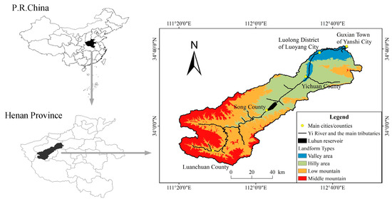
Figure 1.
The location and elevation of the Yi River watershed in China.
The precipitation in the Yi River watershed progressively decreases from the southwest to the northeast with an average precipitation of 700–900 mm. The majority of precipitation occurs in the period from June to August. Torrential rain frequently occurs during this period, which is also known as the high water period.
2.2. Data Resources
The topographic data include DEM data (with 30 m precision) of the Central Plains Economic Zone of China, which were obtained from the National Science and Technology Infrastructure Centre—National Earth System Science Data Sharing Infrastructure—Data Center of Lower Yellow River Regions.
Landscape data included remote sensing images (with 30 m precision) from Landsat-7 that cover the Yi River watershed area. These were obtained in March 2017 (cloudiness of 0.58%). The images were processed and interpreted using ENVI 5.3 (Harris Geospatial Solutions Inc., Broomfield, CO, USA) software to determine the landscape pattern of the Yi River watershed (Figure 2).
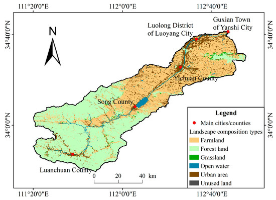
Figure 2.
Main landscape composition types in the Yi River watershed.
For the collection of surface water samples, 42 sampling sites were set on the main stream and major tributaries of the Yi River (Figure 3). The installation of the sampling sites followed the principles that the underlying surface must be similar and the location should be the representative regions of the study area. Samples were collected six times from October 2016 to August 2017: Twice during the drought period (October to December), twice during the ordinary period (March to May), and twice during the high-water period (June to August). At each sampling site, water from the surface layer (0.5 m) was collected and stored in a preprocessed plastic bottle. The situation of the surroundings was recorded. All samples were brought back for laboratory examinations as soon as possible. Before that, they were kept in a cold and dark location.

Figure 3.
Surface water sampling sites.
To determine the water quality indicators, we selected five indicators of surface water quality in this study: Chemical oxygen demand (COD), ammonia nitrogen (NH3–N), total phosphorus (TP), dissolved oxygen (DO), and electrical conductivity (EC). We selected these indicators because the water pollutants in the study area mainly include municipal sewage, chemical sewage, and agricultural non-point source pollution. Thus, the surface water quality in the study area can be fully reflected by these indicators. The DO and EC values were measured in situ using a portable instrument (SX713-02, Runsun Instruments Inc., Chengdu, China). COD, NH3–N, and TP values were determined using an integrated-triple-parameter water quality tester (Lianhua 5B-6C, Lianhua and Technology Inc., Beijing, China). All laboratory experiments were completed in the College of Environment and Planning, Henan University, China. The experimental procedures to determine COD, NH3–N, and TP are described in the following section.
The potassium dichromate (K2Cr2O7) method was applied to determine the COD. This method involves the use of a strong acid solution where a given mass of K2Cr2O7 can oxidize reducing substances in the surface water samples. A ferrous indicator solution is added to an excessive amount of K2Cr2O7 and titrated with an ammonium ferrous sulfate solution. Based on the dosage of ammonium ferrous sulfate, we can calculate the amount of material required to restore the volume of oxygen consumption using the following formula:
where C is the concentration of the ammonium ferrous sulfate standard solution (mol/L); V0 and V1 are the dosages of the ammonium ferrous sulfate standard solution when titrating the blanks (mL) and the surface water samples (mL), respectively; V is the volume of the surface water sample (mL); and 8 is the molar mass (g/mol) of oxygen (1/2O).
CODCr (O2, mg/L) = [(V0 − V1) × C × 8 × 1000]/V
Nessle’s reagent photometry was used to determine NH3–N, which involves the use of the flocculate precipitate to preprocess surface water samples. We absorbed 0, 0.50, 1.00, 3.00, 5.00, 7.00, and 10.00 mL of surface water samples separately into 50 mL colorimetric tubes after the calibration curve was drawn. We diluted the absorbed surface water samples to the marked line before adding 1.0 mL of the potassium sodium tartrate solution. After blending these two solutions, we added 1.5 mL of Nessler’s reagent before blending again. We let this mixture sit for 10 min and then measured the absorbance at a wavelength of 420 nm using the cuvette with 20 mm optical distances. By subtracting the absorbance of the blanks from the determined absorbance, we determined the content of NH3–N (mg) from the calibration curve before calculating the concentration of NH3–N using the following formula:
where m is the content of NH3–N from the calibration curve (mg) and V is the volume of the surface water sample (mL).
NH3–N (N, mg/L) = (m/V) × 1000
The Mo antimony anti-spectrophotometric method is used to determine TP. The experimental procedure is similar to the Nessle’s reagent photometry method. This method involves the use of potassium persulfate digestion to preprocess surface water samples. After the coloration and determination, the content of phosphorus can be calculated from the calibration curve. Finally, the concentration of TP can be calculated by the following formula:
where m is the content of phosphate from the calibration curve (μg) and V is the volume of the surface water sample (mL).
Phosphate (P, mg/L) = m/V
2.3. Analytical Methods
In this study, landscape indices analysis, mapping analysis, principal component analysis (PCA), correlation analysis, and redundancy analysis (RDA) were used. These analyses were completed in FRAGSTATS 4.2 (UMass Landscape Ecology Lab, Amherst, MA, USA), ArcMap 10.3 (Esri Inc., Redlands, CA, USA), SPSS 20.0 (IBM, Armonk, NY, USA), and Canoco 4.5 software (Wageningen University and Research, Wageningen, the Netherlands), respectively.
2.3.1. Landscape Indices Analysis
We considered the sampling sites as the center and set buffer zones in 200 m, 600 m, 1000 m, 1500 m, and 2000 m radii around each sampling site. We selected the radii of buffer zones based on previous literature, which set the smallest radius to 100 m and the largest radius between 1000 m and 2000 m [20].
FRAGSTATS 4.2 (UMass Landscape Ecology Lab, Amherst, MA, USA) software was used to calculate the landscape indices of each buffer zone only at the class level. According to the descriptions and meanings of landscape indices from the software instructions, the selected metrics were total (class) area (CA), percentage of landscape (PLAND), largest path index (LPI), number of patches (NP), contiguity index (CONTIG), patch cohesion index (COHESION), aggregation index (AI), and landscape division index (DIVISION) (Table 1). Within these metrics, CA, PLAND, and LPI are landscape indices that reflect landscape composition, and NP, CONTIG, COHESION, AI, and DIVISION are landscape indices that reflect landscape configuration.

Table 1.
Abbreviations, descriptions, and meanings of the selected landscape indices.
2.3.2. Mapping Analysis
Mapping analysis can be used to visualize the spatial characteristics of surface water quality. Based on the values of surface water quality indicators, the inverse distance weighting (IDW) method was used to interpolate the average concentrations of each indicator within the whole watershed area [20,21,22].
2.3.3. PCA
Using PCA to analyze the surface water quality indicators can simplify multiple indices into a comprehensive index. By combining these results with those from the mapping analysis, the general status of the surface water quality in the watershed area could be presented clearly.
2.3.4. Correlation Analysis
Correlation analysis was completed between the landscape indices and the surface water quality indicators, which allowed us to explore the correlation between landscape patterns and surface water quality.
2.3.5. RDA
RDA can be used to determine the reason why the original variables begin to change. Before undertaking RDA, a detrended correspondence analysis (DCA) must be completed to calculate the gradient and length of the sort axis. RDA can be used when the DCA result is less than 3.
3. Results
3.1. Landscape Indices Analysis
The landscape indices were analyzed at the class level. The results of CA and PLAND show that within the 200 m radius buffer zones, urban area and open water occupy a large proportion of the area, above 70%. Within the 600 m radius buffer zones, the proportions of urban area and farmland are larger, at 39% and 28%, respectively. Within the 1000 m, 1500 m, and 2000 m radius buffer zones, urban area and forest land are the dominant landscape composition types, which together occupy nearly 70% of the total area of buffer zones. Generally, grassland area was the lowest and its proportion in the 200 m radius buffer zones was less than 0.1%. In contrast, the largest proportion of grassland of 1.7% was found within the 600 m radius buffer zones (Figure 4).
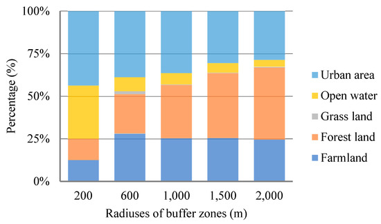
Figure 4.
Proportion of the area of landscape composition types in the total buffer zone area with each radius.
The statistics of the other landscape indices show that the variation in LPI indicates that the urban area is the dominant landscape composition type in the study area. LPI had the largest value within the 600 m radius buffer zones and its largest patch occupies over 80% of the total area of the buffer zones. Apart from grassland, the NP values of all other landscape composition types increased when the radius enlarged. The variations in CONTIG, COHESION, and AI of farmland, forest land, open water, and urban area were similar, which all decreased when the radius increased. The DIVISION values of different landscape composition types varied considerably. The DIVISION values of farmland, open water, and urban area increased when the radius enlarged, whereas that of forest land followed an opposite trend. DIVISION of grassland did not obviously change as the area of grassland was quite small and its patches were too decentralized (Figure 5).
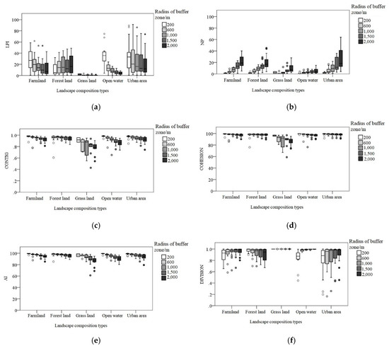
Figure 5.
Statistics of landscape indices in buffer zone with different radiuses: (a) Largest path index (LPI), (b) number of patches (NP), (c) contiguity index (CONTIG), (d) patch cohesion index (COHESION), (e) aggregation index (AI), and (f) landscape division index (DIVISION) values of different landscape composition types.
3.2. Spatial Distribution of Surface Water Quality
The experimental data for each surface water quality indicator were used in a one-sample Kolmogorov–Smirnov (KS) test before use. The results showed that the experimental data all have a normal logarithmic distribution, except for the DO values from the first in situ determination during the drought period and NH3–N values from the second laboratory experiment during the ordinary period. The experimental data were averaged to obtain the values of the surface water quality indicators at each sampling site. IDW was used to interpolate the surface water quality indicators in ArcMap 10.3 (Esri Inc., Redlands, CA, USA) (Figure 6).
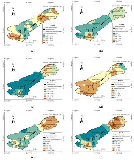
Figure 6.
Spatial heterogeneous distribution of surface water quality indicators in the Yi River watershed: (a) Chemical oxygen demand (COD), (b) ammonia nitrogen (NH3–N), (c) total phosphorus (TP), (d) dissolved oxygen (DO), (e) electrical conductivity (EC), and (f) the spatial distribution of the score of the comprehensive principal components, which can indicate general surface water quality.
After this, we used the Kauser–Meyer–Olkin (KMO) test on the five indicators. The results indicate that the KMO value was 0.753 and the correlating factors between any two surface water quality indicators were mostly above 0.3, which meant that factor analysis could be applied. PCA was used after standardizing the experimental data of the surface water quality indicators, which had a variance contribution rate of 85.4% (Table 2). Therefore, two principal components were extracted. We calculated the scores of the two principal components of each sampling site using Equation (4) to represent the general surface water quality in the study area:
Table 2.
The capacity and variance contribution rate of the principal components.
After this, we used the same method to visualize the spatial distribution of general surface water quality using ArcMap 10.3 (Esri Inc., Redlands, CA, USA) (Figure 6).
The results indicate that, in general, the surface water quality around Song County is the best. In the southwest, the precipitous landform causes pollutants from the soil and surrounding environment to flow into water bodies, especially in places near Luchuan County. In the northeast, a greater area is covered by urban area and farmland, which are sources of increased pollution that worsen the surface water quality.
3.3. Correlation Between Landscape Patterns and Surface Water Quality
3.3.1. Landscape Composition and Surface Water Quality
Correlation analysis showed that the PLAND of farmland was significantly negatively correlated (p < 0.05) with TP and DO concentrations within the 1500 m radius buffer zones. LPI began to have a significant positive correlation (p < 0.01) with EC when the radius of the buffer zone was larger than 1500 m. Within the 200 m radius buffer zones, PLAND and LPI of forest land had significant negative correlations (p < 0.05) with COD concentration, and LPI had a significant positive correlation with EC (p < 0.05). The landscape indices of grassland had no significant correlation with any surface water quality indicators, as the area of grassland was quite small in the study area. For the urban area, PLAND had significant positive correlations (p < 0.05) with COD, TP, EC, and the general surface water quality in 2000 m radius buffer zones. LPI also had significant positive correlations with NH3–N, TP, EC, and the general surface water quality within 2000 m radius buffer zones (Table 3).
Table 3.
Correlations between PLAND, LPI, and surface water quality indicators.
3.3.2. Landscape Configuration and Surface Water Quality
The results from the Spearman correlation analysis indicated that when the radius of buffer zones is small, only forest land is correlated to the surface water quality indicators. In contrast, when the radius of buffer zones is large, only the urban area is correlated with the surface water quality indicators. In the 200 m radius buffer zones, the landscape configuration indices of forest land were mostly correlated with COD. COD concentration had significant negative correlations with CONTIG, COHESION, and AI (p < 0.05) and a significant positive correlation with DIVISION (p < 0.05). TP concentration had a stronger significant negative correlation with NP (p < 0.01) and a positive correlation with EC (p < 0.05) (Table 4).
Table 4.
Correlations between landscape configuration indices of forest land and surface water quality indicators (200 m radius).
In the 2000 m radius buffer zones, the urban area had significant correlations with NH3–N, TP, EC, and the general surface water quality. NH3–N had a significant positive correlation with the COHESION of the urban area and significant negative correlations with NP and DIVISION (p < 0.05). NH3–N had no correlating relationships with CONTIG and AI. TP had significant correlations with all landscape configuration indices, significant negative correlations with NP and DIVISION (p < 0.01), and significant positive correlations with CONTIG and COHESION (p < 0.01). COD and DO had no correlations with the landscape indices of urban areas. EC had significant positive correlating relationships with CONTIG and AI (p < 0.05) and significant negative correlations with NP and DIVISION (p < 0.05). In general, the urban area in the 2000 m radius buffer zones had the greatest impact on the general surface water quality as their correlation was relatively high (Table 5).
Table 5.
Correlations between landscape configuration indices of the urban area and surface water quality indicators (2000 m radius).
3.4. Impacting Strengths of Landscape Composition and Configuration on Surface Water Quality
RDA was used to explore the impacting strengths of landscape composition and configuration on the surface water quality using Canoco 4.5 (Wageningen University and Research, Wageningen, The Netherlands). The values of the landscape indices in the 2000 m radius buffer zones and experimental data of surface water quality indicators were applied to run the RDA. The results showed that the accumulating contribution rates of axis 1 and axis 2 were more than 98%, which indicated that RDA can explicitly reflect the relationships between surface water quality indicators and landscape indices (Table 6).
Table 6.
Redundancy analysis (RDA) results of landscape indices and surface water quality indicators.
The degrees of the included angle cosine and the lengths of the arrows can show the correlation and the influencing strength among the indicators. When the degrees of the included angle between two indicators are less than 90°, it means these two indicators have positive correlations. When the degree of the included angle between two indicators is more than 90°, it means these two indicators have negative correlations. The length of the arrow represents the percentage that is shared by the influencing factor, a longer arrow signifies a stronger influencing strength. To decide, the RDA ordination showed that in the 2000 m radius buffer zones the surface water quality was affected by NP, CA, and PLAND, which means that landscape compositional change influences surface water quality more than landscape configurational change (Figure 7).
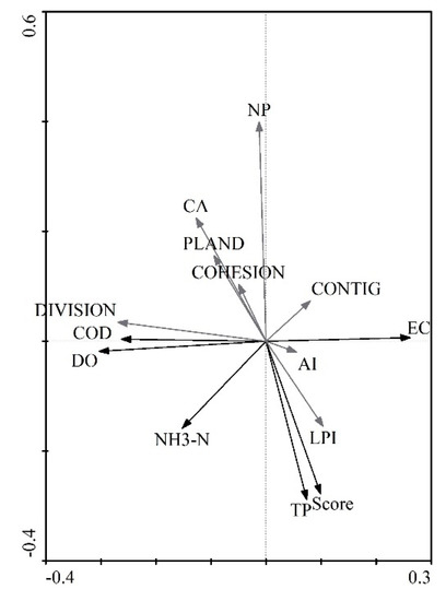
Figure 7.
RDA ordination of landscape indices and surface water quality indicators.
4. Discussion
Surface water quality is a comprehensive representation of the surrounding environment thus, the spatial-temporal variation in landscape patterns can cause changes in the surface water quality. Therefore, we discussed the effects of variation in landscape on surface water quality.
4.1. Effects of Landscape Composition on Surface Water Quality
Landscape composition reflects the non-spatial characteristics of the landscape. The results showed that when the areas of some landscape composition types increase, surface water quality improves. In contrast, for some other landscape composition types, the result is the inverse.
With the change in the radius of buffer zones, different landscape composition types have different correlations with surface water quality indicators. As a ‘sink’ landscape composition type, forest land can effectively improve the quality of surface water flow by absorbing pollutants [17,25,26]. In this study, when forest land was near water bodies, its landscape compositional changed: The area, patch numbers, or the largest patch area increased, which decreased concentrations of COD and TP. This conclusion confirms the findings of previous studies [21,27,28,29]. The soil and plants in forest land can effectively reduce storm run-off, water loss, and soil erosion, as well as absorb pollutants, which prevent organic matter and nutrients from penetrating into water bodies through surface water flow.
When the buffer zones have a larger radius, a greater proportion is in the urban area, and the urban area has considerable effects on surface water quality. When the urban area increases, concentrations of COD and TP also grow. The largest urban patch area can affect concentrations of NH3–N and TP, which are positively correlated. This indicates that a greater proportion of the urban area could cause an increase in surface water pollution because the impervious surface in urban areas results in pollutants draining into water bodies through surface water flow [3,30,31].
Farmland is the landscape composition type that experiences frequent human disturbance. The effects of farmland on the surface water quality are quite complex. Fertilization results in nutrients flowing into water bodies. However, the plants in farmland and the paddy field can stop and absorb some water pollutants. In this study, when the area of farmland increased, the concentration of TP decreased, which aligns with the results of existing studies [5,23].
4.2. Effects of Landscape Configuration on Surface Water Quality
The spatial distribution and the configuration of landscape composition types can directly impact surface water quality. However, only a few studies have linked landscape configuration and surface water quality.
In this study, forest configuration change was found to effectively influence the surface water quality. When the patches of forest land were aggregative or the trend in area was increasing, the patches had an intensive configuration and the connectivity among patches was good. This improves the purifying effect of the forest on the surface water quality. However, urban area configurational change was the most important factor affecting surface water quality and concentrations of NH3–N and TP more significantly responded to its variation [3,15,25]. When the urban area configuration becomes intensive, such as places near Luanchuan County and Yichuan County, the splitting degree of patches is low and urban area becomes the dominant landscape type. This would increase the concentration of domestic sewage and concentrations of NH3–N and TP. Thus, the surface water quality would be significantly reduced.
5. Conclusions
We analyzed surface water quality indicators and their spatial distribution in the Yi River watershed in China through the use of in situ and laboratory experiments as well as geostatistics models. The landscape patterns of the study area were analyzed by setting buffer zones with different radii from the river sampling points. We discussed how a change in landscape patterns would affect the surface water quality from two aspects: Landscape composition and landscape configuration. We compared the impacting strengths of landscape composition and configuration on surface water quality. The results showed that: (1) We can control the COD concentration by increasing the forest land area, which means that creating forest land near water bodies can effectively decrease non-point source pollution, (2) the increase in urban area is the main factor negatively impacting surface water quality, and (3) landscape compositional change has greater influence than landscape configurational change on surface water quality.
Author Contributions
Conceptualization, Z.B. and S.D.; methodology, L.L.; software, L.L.; validation, Z.B., L.L., and S.D.; formal analysis, Z.B.; investigation, Z.B., L.L., and S.D.; resources, Z.B.; data curation, L.L.; writing—original draft preparation, Z.B.; writing—review and editing, L.L. and S.D.; visualization, Z.B. and L.L.; supervision, S.D.; project administration, S.D.; funding acquisition, S.D.
Funding
This research was funded by National Natural Science Foundation of China, grant number 41771202.
Acknowledgments
The authors thank the National Earth System Science Data Sharing Service Platform—the Lower Yellow River Science Data Centre (http://henu.geodata.cn) for the data support.
Conflicts of Interest
The authors declare no conflict of interest.
References
- Shi, P.; Zhang, Y.; Li, Z.; Li, P.; Xu, G. Influence of land use and land cover patterns on seasonal water quality at multi-spatial scales. Catena 2017, 151, 182–190. [Google Scholar] [CrossRef]
- Fu, B.; Chen, L.; Ma, K. The effect of land use Chang on the regional environment in the Yangjuangou catchment in the Loess Plateau of China. Acta Geogr. Sin. 1999, 54, 241–246. [Google Scholar]
- Yang, J.; Xu, Y.; Gao, B.; Wang, Y.; Xu, Y.; Ma, Q. River water quality change and its relationship with landscape pattern under the urbanization: A case study of Suzhou City in Taihu Basin. J. Lake Sci. 2017, 29, 827–835. [Google Scholar]
- Lawler, J.J. Landscape pattern and ecological process: An important update of a classic textbook. Ecology 2017, 98, 2231–2232. [Google Scholar] [CrossRef]
- Lee, S.; Hwang, S.; Lee, S.; Hwang, H.; Sung, H. Landscape ecological approach to the relationships of land use patterns in watersheds to water quality characteristics. Landsc. Urban Plan. 2009, 92, 80–89. [Google Scholar] [CrossRef]
- McGrane, S.J. Impacts of urbanization on hydrological and water quality dynamics and urban water management: A review. Hydrol. Sci. J. J. Sci. Hydrol. 2016, 61, 2295–2311. [Google Scholar] [CrossRef]
- Janardan, M.; Heejun, C. Landscape and anthropogenic factors affecting spatial patterns of water quality trends in a large river basin, South Korea. J. Hydrol. 2018, 564, 26–40. [Google Scholar]
- Wang, X.; Zhang, F.; Li, X.; Cao, C.; Guo, M.; Chen, L. Correlation analysis between the spatial characteristics of land use/cover-landscape patter and surface-water quality in the Ebinur Lake area. Acta Ecol. Sin. 2017, 37, 7438–7452. [Google Scholar]
- Ji, D.; Wen, Y.; Wei, J.; Wu, Z.; Liu, Q.; Cheng, J. Relationships between landscape spatial characteristics and surface water quality in the Liu Xi River watershed. Acta Ecol. Sin. 2015, 35, 246–253. [Google Scholar]
- Tscharntke, T.; Batáry, P.; Dormann, C.F. Set-aside management: How do succession, sowing patterns and landscape context affect biodiversity? Agric. Ecosyst. Environ. 2011, 143, 37–44. [Google Scholar] [CrossRef]
- Prager, K.; Reed, M.; Scott, A. Encouraging collaboration for the provision of ecosystem services at a landscape scale—Rethinking agri-environmental payments. Land Use Policy 2012, 29, 244–249. [Google Scholar] [CrossRef]
- Beck, S.M.; Mchale, M.R.; Hess, G.R. Beyond impervious: Urban land-cover pattern variation and implications for watershed management. Environ. Manag. 2016, 58, 15–30. [Google Scholar] [CrossRef] [PubMed]
- Wu, J.; Guo, X.; Yang, Y.; Qian, G.; Niu, J.; Liang, C.; Zhang, Q.; Li, A. What is sustainability science? Chin. J. Appl. Ecol. 2014, 25, 1–11. [Google Scholar]
- Qiu, J.; Turner, M.G. Importance of landscape heterogeneity in sustaining hydrologic ecosystem services in an agricultural watershed. Ecosphere 2015, 6, 1–19. [Google Scholar] [CrossRef]
- Peng, J.; Du, Y.; Liu, Y.; Wu, J.; Wang, Y. From natural regionalization, land change to landscape service: The development of integrated physical geography in China. Geogr. Res. 2017, 36, 1819–1833. [Google Scholar]
- Sabit, M.; Nasirdin, N.; Mamut, A. Analysis on the change in land use/cover ecological service value in Tomur National Reserve. Geogr. Res. 2016, 35, 2116–2124. [Google Scholar]
- Xia, P.; Kong, X.; Yu, L. Effects of land-use and landscape pattern on nitrogen and phosphorus exports in Caohai wetland watershed. Acta Sci. Circumst. 2016, 36, 2983–2989. [Google Scholar]
- Zhang, Y.; Chen, S.; Xiang, J. Correlation between the water quality and land use composition in the river side area—A case of Chaohu Lake basin in China. Resour. Environ. Yangtze Basin 2011, 20, 1054–1061. [Google Scholar]
- Jung, K.; Lee, S.; Hwang, H.; Jang, J. The effects of spatial variability of land use on stream water quality in a costal watershed. Paddy Water Environ. 2008, 6, 275–284. [Google Scholar] [CrossRef]
- Uriarte, M.; Yackulic, C.B.; Lim, Y.; Arce-Nazario, J.A. Influence of land use on water quality in a tropical landscape: A multi-scale analysis. Landsc. Ecol. 2011, 26, 1151–1164. [Google Scholar] [CrossRef]
- Cai, H.; Lin, G.; Kang, W. The effects of sloping landscape features on water quality in the upper and middle reaches of the Chishui River Watershed. Geogr. Res. 2018, 37, 704–716. [Google Scholar]
- Roces-Díaz, J.V.; Vayreda, J.; Banqué-Casanovas, M.; Díaz-Varela, E.; Bonet, J.A.; Brotons, L.; de-Miguel, S.; Herrando, S.; Martínez-Vilaltaah, J. The spatial level of analysis affects the patterns of forest ecosystem services supply and their relationships. Sci. Total Environ. 2018, 626, 1270–1283. [Google Scholar] [CrossRef] [PubMed]
- Billmire, M.; Koziol, B.W. Landscape and flow path-based nutrient loading metrics for evaluation of in-stream water quality in Saginaw Bay, Michigan. J. Gt. Lakes Res. 2018, 44, 1068–1080. [Google Scholar] [CrossRef]
- Teixeira, D.G.; Marques, S.P.; Garabini, C.T.; Ribeiro, M.C.; Paglia, A.P. The effects of landscape patterns on ecosystem services: Meta-analyses of landscape services. Landsc. Ecol. 2018, 33, 1247–1257. [Google Scholar]
- Basnyat, P.; Teeter, L.D.; Flynn, K.M.; Lockaby, B.G. Relationships between landscape characteristics and nonpoint source pollution inputs to coastal estuaries. Environ. Manag. 1999, 23, 539–549. [Google Scholar] [CrossRef]
- Tong, S.T.Y.; Chen, W. Modeling the relationship between land use and surface water quality. J. Environ. Manag. 2002, 66, 377–393. [Google Scholar] [CrossRef]
- Qiu, J.; Turner, M.G. Spatial interactions among ecosystem services in an urbanizing agricultural watershed. Proc. Natl. Acad. Sci. USA 2013, 110, 12149–12154. [Google Scholar] [CrossRef] [PubMed]
- Zhang, D.; Li, Y.; Sun, X.; Zhang, F.; Zhu, H.; Liu, Y.; Zhang, Y.; Zhuang, M.; Zhu, X. Relationship between landscape pattern and river water quality in Wujingang region, Taihu Lake watershed. Environ. Sci. 2010, 31, 1775–1783. [Google Scholar]
- King, R.S.; Baker, M.E.; Whigham, D.F.; Weller, D.E.; Jordan, T.E.; Hurd, K.M.K. Spatial considerations for linking watershed land cover to ecological indicators in streams. Ecol. Appl. 2005, 15, 137–153. [Google Scholar] [CrossRef]
- Yu, S.; Jiang, M.; Yuan, Y. Spatial heterogeneity of water quality in Xiaoxingkai Lake. Wetl. Sci. 2015, 13, 166–170. [Google Scholar]
- Zhang, L.; Mou, Z.; Sun, H.; Zhang, Z. Spatial and temporal variability of water quality of city river in south Jiangsu. Environ. Pollut. Control. 2012, 34, 28–33. [Google Scholar]
© 2019 by the authors. Licensee MDPI, Basel, Switzerland. This article is an open access article distributed under the terms and conditions of the Creative Commons Attribution (CC BY) license (http://creativecommons.org/licenses/by/4.0/).