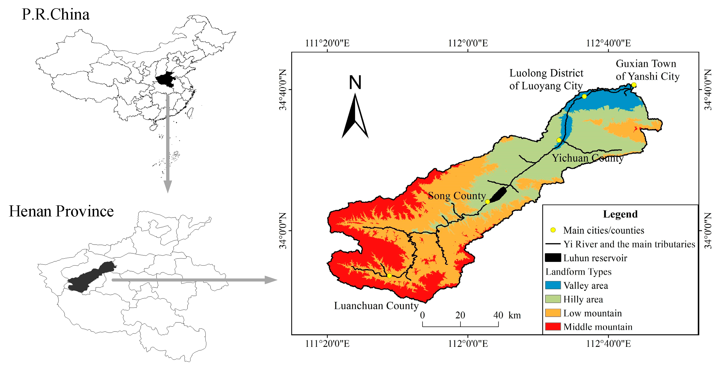
2.1. Site Description
The Yi River is one of the major branches of the Yellow River in China. The Yi River flows from southwest to northeast and runs through Luanchuan County, Song County, Yichuan County, Luolong District of Luoyang City, and Yanshi City in the Henan Province. The overall length of the main stream of the Yi River is 242.4 km. Based on the digital elevation model (DEM) data (with a precision of 30 m) of the Central Plains Economic Zone of China, the extent of the Yi River watershed was generated using the soil and water assessment tool (SWAT) in ArcGIS (Esri Inc., Redlands, CA, USA) (111°19′–112°55′ E, 33°39′–34°41′ N). The total area of the Yi River watershed is 5937 km
2 and the elevation is 110–2200 m. The natural features of the Yi River watershed include the middle-mountain, low-mountain, hilly area, and valley (
Figure 1). The proportion of the mountainous area is 50%, the hilly area is 40%, and the valley is 10%. The main landscape composition types in the Yi River watershed are farmland, forest land, grassland, open water, and urban area (
Figure 1).
The precipitation in the Yi River watershed progressively decreases from the southwest to the northeast with an average precipitation of 700–900 mm. The majority of precipitation occurs in the period from June to August. Torrential rain frequently occurs during this period, which is also known as the high water period.
2.2. Data Resources
The topographic data include DEM data (with 30 m precision) of the Central Plains Economic Zone of China, which were obtained from the National Science and Technology Infrastructure Centre—National Earth System Science Data Sharing Infrastructure—Data Center of Lower Yellow River Regions.
Landscape data included remote sensing images (with 30 m precision) from Landsat-7 that cover the Yi River watershed area. These were obtained in March 2017 (cloudiness of 0.58%). The images were processed and interpreted using ENVI 5.3 (Harris Geospatial Solutions Inc., Broomfield, CO, USA) software to determine the landscape pattern of the Yi River watershed (
Figure 2).
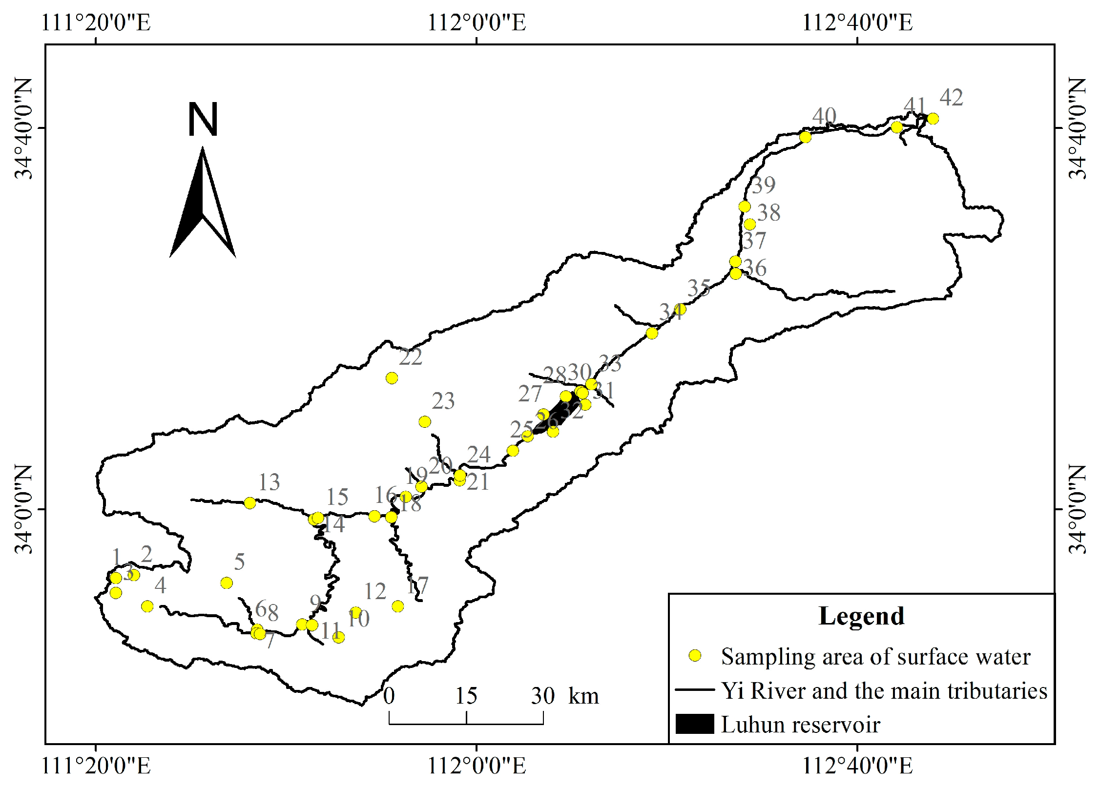
For the collection of surface water samples, 42 sampling sites were set on the main stream and major tributaries of the Yi River (
Figure 3). The installation of the sampling sites followed the principles that the underlying surface must be similar and the location should be the representative regions of the study area. Samples were collected six times from October 2016 to August 2017: Twice during the drought period (October to December), twice during the ordinary period (March to May), and twice during the high-water period (June to August). At each sampling site, water from the surface layer (0.5 m) was collected and stored in a preprocessed plastic bottle. The situation of the surroundings was recorded. All samples were brought back for laboratory examinations as soon as possible. Before that, they were kept in a cold and dark location.
To determine the water quality indicators, we selected five indicators of surface water quality in this study: Chemical oxygen demand (COD), ammonia nitrogen (NH3–N), total phosphorus (TP), dissolved oxygen (DO), and electrical conductivity (EC). We selected these indicators because the water pollutants in the study area mainly include municipal sewage, chemical sewage, and agricultural non-point source pollution. Thus, the surface water quality in the study area can be fully reflected by these indicators. The DO and EC values were measured in situ using a portable instrument (SX713-02, Runsun Instruments Inc., Chengdu, China). COD, NH3–N, and TP values were determined using an integrated-triple-parameter water quality tester (Lianhua 5B-6C, Lianhua and Technology Inc., Beijing, China). All laboratory experiments were completed in the College of Environment and Planning, Henan University, China. The experimental procedures to determine COD, NH3–N, and TP are described in the following section.
The potassium dichromate (K
2Cr
2O
7) method was applied to determine the COD. This method involves the use of a strong acid solution where a given mass of K
2Cr
2O
7 can oxidize reducing substances in the surface water samples. A ferrous indicator solution is added to an excessive amount of K
2Cr
2O
7 and titrated with an ammonium ferrous sulfate solution. Based on the dosage of ammonium ferrous sulfate, we can calculate the amount of material required to restore the volume of oxygen consumption using the following formula:
where
C is the concentration of the ammonium ferrous sulfate standard solution (mol/L);
V0 and
V1 are the dosages of the ammonium ferrous sulfate standard solution when titrating the blanks (mL) and the surface water samples (mL), respectively;
V is the volume of the surface water sample (mL); and 8 is the molar mass (g/mol) of oxygen (1/2O).
Nessle’s reagent photometry was used to determine NH
3–N, which involves the use of the flocculate precipitate to preprocess surface water samples. We absorbed 0, 0.50, 1.00, 3.00, 5.00, 7.00, and 10.00 mL of surface water samples separately into 50 mL colorimetric tubes after the calibration curve was drawn. We diluted the absorbed surface water samples to the marked line before adding 1.0 mL of the potassium sodium tartrate solution. After blending these two solutions, we added 1.5 mL of Nessler’s reagent before blending again. We let this mixture sit for 10 min and then measured the absorbance at a wavelength of 420 nm using the cuvette with 20 mm optical distances. By subtracting the absorbance of the blanks from the determined absorbance, we determined the content of NH
3–N (mg) from the calibration curve before calculating the concentration of NH
3–N using the following formula:
where
m is the content of NH
3–N from the calibration curve (mg) and
V is the volume of the surface water sample (mL).
The Mo antimony anti-spectrophotometric method is used to determine TP. The experimental procedure is similar to the Nessle’s reagent photometry method. This method involves the use of potassium persulfate digestion to preprocess surface water samples. After the coloration and determination, the content of phosphorus can be calculated from the calibration curve. Finally, the concentration of TP can be calculated by the following formula:
where
m is the content of phosphate from the calibration curve (μg) and
V is the volume of the surface water sample (mL).
2.3. Analytical Methods
In this study, landscape indices analysis, mapping analysis, principal component analysis (PCA), correlation analysis, and redundancy analysis (RDA) were used. These analyses were completed in FRAGSTATS 4.2 (UMass Landscape Ecology Lab, Amherst, MA, USA), ArcMap 10.3 (Esri Inc., Redlands, CA, USA), SPSS 20.0 (IBM, Armonk, NY, USA), and Canoco 4.5 software (Wageningen University and Research, Wageningen, the Netherlands), respectively.
2.3.1. Landscape Indices Analysis
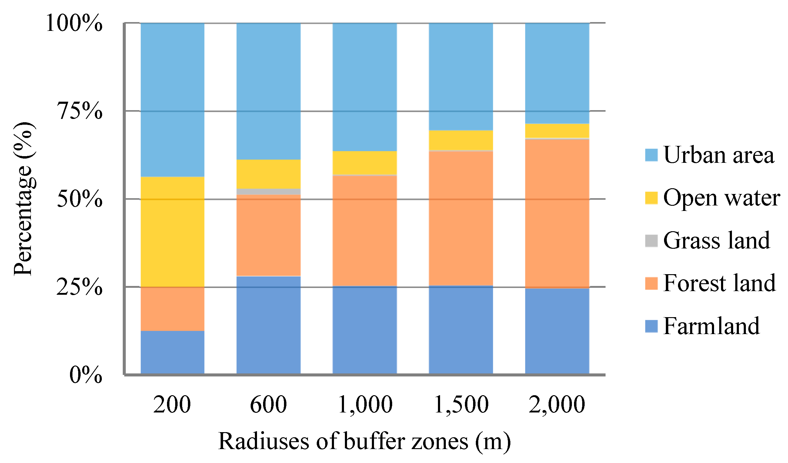
We considered the sampling sites as the center and set buffer zones in 200 m, 600 m, 1000 m, 1500 m, and 2000 m radii around each sampling site. We selected the radii of buffer zones based on previous literature, which set the smallest radius to 100 m and the largest radius between 1000 m and 2000 m [
20].
FRAGSTATS 4.2 (UMass Landscape Ecology Lab, Amherst, MA, USA) software was used to calculate the landscape indices of each buffer zone only at the class level. According to the descriptions and meanings of landscape indices from the software instructions, the selected metrics were total (class) area (
CA), percentage of landscape (
PLAND), largest path index (
LPI), number of patches (
NP), contiguity index (
CONTIG), patch cohesion index (
COHESION), aggregation index (
AI), and landscape division index (
DIVISION) (
Table 1). Within these metrics,
CA,
PLAND, and
LPI are landscape indices that reflect landscape composition, and
NP,
CONTIG,
COHESION,
AI, and
DIVISION are landscape indices that reflect landscape configuration.
2.3.2. Mapping Analysis
Mapping analysis can be used to visualize the spatial characteristics of surface water quality. Based on the values of surface water quality indicators, the inverse distance weighting (IDW) method was used to interpolate the average concentrations of each indicator within the whole watershed area [
20,
21,
22].
2.3.3. PCA
Using PCA to analyze the surface water quality indicators can simplify multiple indices into a comprehensive index. By combining these results with those from the mapping analysis, the general status of the surface water quality in the watershed area could be presented clearly.
2.3.4. Correlation Analysis
Correlation analysis was completed between the landscape indices and the surface water quality indicators, which allowed us to explore the correlation between landscape patterns and surface water quality.
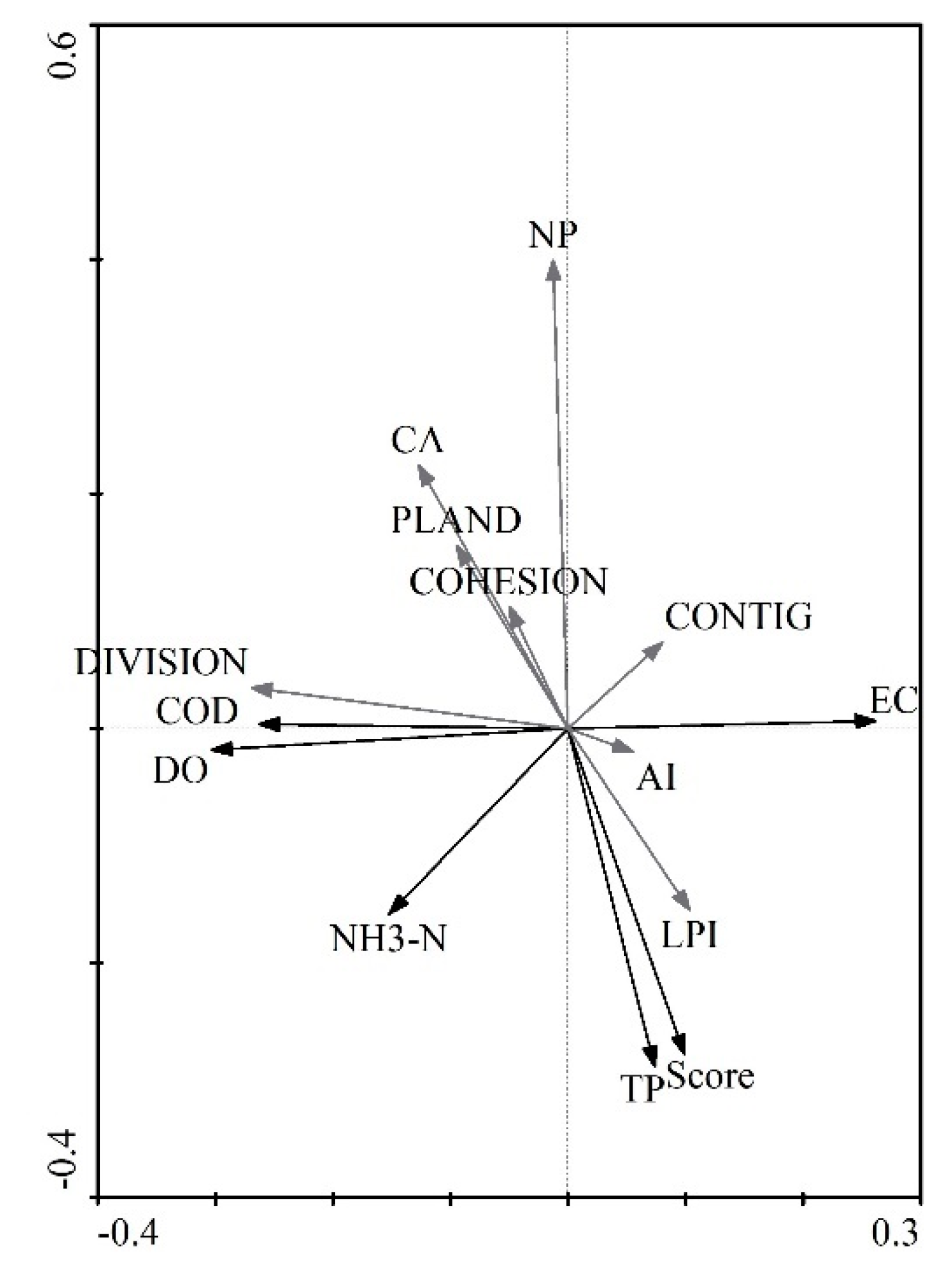
2.3.5. RDA
RDA can be used to determine the reason why the original variables begin to change. Before undertaking RDA, a detrended correspondence analysis (DCA) must be completed to calculate the gradient and length of the sort axis. RDA can be used when the DCA result is less than 3.


