Article

Coal Seam Thickness Prediction Based on Transition Probability of Structural Elements

1
School of Computer Science and Technology, Xi’an University of Science and Technology, Xi’an 710054, China
2
Beijing Key Lab of Human-Computer Interaction, Institute of Software, Chinese Academy of Sciences, Beijing 100190, China
3
University of Chinese Academy of Sciences, Beijing 100049, China
4
General Engineering Research Institute, Faculty of Engineering and Technology, Liverpool John Moores University, Byrom Street, Liverpool L3 3AF, UK
*
Author to whom correspondence should be addressed.
Appl. Sci. 2019, 9(6), 1144; https://doi.org/10.3390/app9061144
Submission received: 25 January 2019 / Revised: 14 March 2019 / Accepted: 14 March 2019 / Published: 18 March 2019

Abstract

:
Coal seam thickness prediction is crucial in coal mine design and coal mining. In order to improve the prediction accuracy, an improved Kriging interpolation method on the basis of efficient data and Radial Basis Function (RBF-Kriging) is firstly proposed to interpolate the cutting data that is obtained in pre-mining, especially at the edge of the geological surface of coal seam by taking into account the spatial structure and the efficient spatial range, ensuring the integrity of the edge data during the movement of structural elements. Subsequently, a structural element transition probability based Gaussian process progression (STTP-GPR) method is proposed to predict the coal seam thickness from the interpolated coal seam data. The experimental results demonstrated that the proposed STTP-GPR method has superior performance in coal seam thickness prediction. The average absolute error of thickness prediction for thin coal seams is 0.025 m, which significantly improves the prediction accuracy in comparison to the existing back propagation (BP) neural networks, support vector machine, and Gaussian process regression methods.

1. Introduction

Coal resource is a valuable non-renewable energy source. The average coal mining rate in China’s large-scale mining areas is about 30% to 40% and the recovery rate for small coal mines is even less than 10% [1]. The low mining rate leads to large waste of resources. At present, the mechanized mining of coal mines is seriously inadequate in China. According to statistics [2], China’s mechanization in key coal mining areas is 75% and the national average mechanization level is less than 40%. Therefore, the development of automatically and intelligently coal mining techniques is an urgent issue to be solved in China.
Due to the rigors of the mining environment and the coal mining safety, the automation technologies are paying great attention at present. The indirect prediction of the entire coal-rock interface is critical in achieving automation and intelligence of coal mining through borehole data and partial mining data. Coal seam thickness is important information in coal mine design and mining. The effective detection of coal-rock interface and accurate prediction of coal seam thickness not only provides the good geology of coalmine, but it is also crucial for high-yield and high-efficiency mining and the automatic height adjustment of the shearer drum at a man-less working face [3]. The cutting data obtained in pre-mining is relatively accurate in the numerous mine geological data, but due to the limited amount of cutting data, an appropriate interpolation method should be adopted in order to predict the complete set of the coal seam thickness data.
Among the large amount of interpolation methods, Kriging interpolation is widely used in the field of coal mining. It takes the spatial correlation into account when dealing with data, achieving good performance in most cases [4].
In the Kriging interpolation, the types of variation function model are finite, which make the variation function very difficult in describing the spatial distribution characteristics of true data. In order to overcome this shortage, an improved interpolation, called Support Vector Machine-Kriging interpolation (SVM-Kriging), was proposed in [5]. The SVM-Kriging uses the Least Square Support Vector Machine (LS-SVM) to fit the variation function and to directly get the optimal variation function for the real interpolated field by using SVM to automatically fit the variation function curve. In [6], the Kriging interpolation method was used to study the coal quality prediction model of cutting coal, and the parameters of the optimal variation function model and experimental variation function are determined based on data characteristics. The spatial distribution of ash and heat is predicted by using the Kriging interpolation method. In [7,8], a method that is based on dimensionless parameters and SVM was proposed for coal-rock interface identification.
In the existing methods, the spatial structure and spatial distribution in the region of the coal seam geology transition are seldom taken into account. Moreover, the coal seam thickness changing is considered only for the marching direction, and the changes in other directions are usually ignored. As a result, the accuracy of coal seam thickness prediction is affected by such simplifications.
In recent years, the Gaussian process (GP) regression has been demonstrated to handle the uncertainty in predictive analytics problems with superior predictive performance. GPs can model complex systems, whilst handling uncertainty in a principled manner. GPs can exploit prior information in a variety of ways: explicit mean functions can be used if the functional form of the underlying degradation model is available, and multiple-output GPs can effectively exploit correlations between data. Ref [9,10] used the Gaussian process regression algorithm for time series prediction and battery life prediction, and various advantages over other data-drive and mechanistic methods were demonstrated.
In this paper, an improved Kriging interpolation method on the basis of efficient data and Radial Basis Function (RBF-Kriging) is firstly proposed to interpolate the borehole data, especially in the transition areas of the geological surface of coal seam to ensure the integrity of the transition data. Subsequently, a structural element transition probability based Gaussian process progression (STTP-GPR) method is proposed to predict the coal seam thickness from the interpolated data. Our method can be used to generate the coal-rock interface and predict the coal seam thickness, where the data will be used to guide the shearer drum to automatically adjust the coal cutting height in automatically and intelligently coal mining.

2. RBF-Kriging for Borehole Data Interpolation

2.1. Ordinary Kriging

The ordinary Kriging interpolation [11] is a spatial interpolation method that was developed based on the Geo-statistical variation function model. Let z ( x i ) be the value of the variable Z at a point x. Given the n measurements Z ( x 1 ) , , Z ( x n ) at the known locations x 1 , , x 2 , the Kriging estimator interpolates an estimate of z ( x 0 ) at an unsampled location x 0 by weighed linear combinations of the available samples:
z ( x 0 ) = i = 0 n λ i z ( x i ) ,
where λ is the interpolation weight. Considering the unbiasedness condition yields:
i = 1 n λ i = 1 .
Since the weighting procedure depends on both the distance and statistical distribution of the samples, the variation function is adopted to estimate the weight by fitting a spatial model to the data and then defining the effectiveness of each point [12,13]. The variation function value at point x i is obtained by
γ ( h ) = 1 2 N ( h ) i = 1 N ( h ) [ z ( x i ) z ( x i + h ) ] 2
where h is the distance between two points, N(h) is the number of pairs separated by h. Therefore, the variation function value γ ( x i x j ) between observation points x i and x j , and the variation function value γ ( x 0 x j ) between the interpolation point x 0 and the observation point x j can be calculated by the fitting function. In general, the fitting function is chosen by experience. The common model includes mainly the linear model, the Gaussian model, and the Exponential model.
The interpolation weight in Equation (1) can be computed by combining Equations (2) and (4):
i = 1 n λ i γ ( x i x j ) + ε = γ ( x 0 x j ) , j = 1 , , n .
where ε is the Lagrange multiplier, which can be calculated as well. ε is introduced to make the variance minimum for the estimate in Equation (1). Subsequently, z ( x 0 ) can be obtained by Equation (1).
Although the Kriging performs well in the coal seam thickness prediction, the variation function model, which is often chosen by experience, may not accurately express the cutting data. In this paper, calculating the interpolation weight using efficient samples and fitting the variation function through RBF improves the Kriging method.

2.2. Efficient Samples

As seen from Section 2.1, for the ordinary Kriging interpolation, each data point that is to be interpolated is calculated through all available samples. According to the first law of geography of “All attribute values on a geographic surface are related to each other, but closer values are more strongly related than are more distant ones”, coal seam thickness at a given data point is more related to its neighborhood. In other words, the samples with the larger weighting coefficients are concentrated around the interpolated point. This property is described by the Gaussian model in the proposed method, as shown in the Equation (5),
f ( x ) = 1 2 π σ e ( x μ ) 2 2 σ 2
which is widely used as the variation function model in the ordinary Kriging, where μ and σ are the mean and variance of the Gaussian distribution and x is the samples. For the Gaussian model, the probability of samples fall within [−3σ, 3σ] is 99.74%, i.e.,
p { | x μ | < 3 σ } = 2 ϕ ( 3 ) 1 = 0.9974 .
In order to ensure that the nearest point has a greater influence on the interpolation point in the Kriging method, the variation function, as shown in Equation (3), is only calculated through the efficient samples. In this paper, the efficient samples are restricted to the samples falling within [−3σ, 3σ] to the interpolated point by experience. Thus, the Kriging linear equations, by which the weight can be calculated, is derived as follows:
{ i = 1 n λ i = 1 i = 1 n λ i γ ( x i , x j ) = γ ( x i , x 0 ) d ( x i , x 0 ) 3 σ
where, d ( x i , x 0 ) represents the distance between observation point and the interpolated point. Notice that the utilization of the efficient samples not only improves the interpolation performance, but also reduces the computational complexity.

2.3. Variation Function Determination Using RBF

In the process of calculating the interpolation weights, the variation function often depends on experience. For the commonly used variation functions such as the linear model, Gaussian model, exponential model, etc., it was shown in practical applications that the relative error is relatively large, the spatial characteristics of the existing sampling points may not be well described by these models, and the integrity of the direction and distance information in the data space cannot be guaranteed [14].
The RBF network has its origin in performing an exact interpolation of a set of data points in a multidimensional space. The RBF network is a universal approximator and it is a popular alternative to the multilayer perception (MLP) neural network, since it has a simpler structure and a much faster training process. It is widely used for classification and function approximation. The RBF network consists of three layers: input layer, hidden layer, and output layer. The input layer is connected to the hidden layer by radial basis functions, and the hidden layer to output layer is connected through a simple weight connection. The Gaussian radial function output from the hidden layer is linearly weighted to generate output. As a result, the RBF network can approximate any function with any required precision. This property has great potential to learn the variation function for Kriging interpolation. Furthermore, the RBF variation function can alleviate the long-distance point interference due to its simple three-layers structure. Finally, normalization is carried out to normalize the distance vector h to keep the distance h and the variation function values γ in the same level of magnitude.
Because of the relationship between the distance and variation function, the variation function must be greater or equal to 0. While using the RBF network to fit the variation function, the value of variation may be less than 0, but the probability is almost 0 as the result of the efficient sample chose at part 1.2. If the value of variation function that is fitted by RBF is less than 0, then we will configure the value as 0, because the distance of two points is too long and the effect of two points at the distance is negligible.

2.4. Implementation of RBF-Kriging

The implementation of the proposed RBF-Kriging interpolation algorithm is summarized, as follows:
  • Step 1: For coal seam data D = { ( l i , w i , z i ) | l i , w i , z i R + , 0 < i n } , calculate the distance of from point x i and point x j ,
    d = ( l i l j ) 2 + ( w i w j ) 2 , 0 < i j n ;
    where l and w is plane coordinates of the location x
  • Step 2: Calculate the variation function values between point pairs as,
    r ( d ) = 1 2 N ( d ) i , j = 1 N ( d ) [ z ( l i , w i ) z ( l j , w j ) ] 2 ,
    and one-to-one correspondence with distance, where,   d = ( l i l j ) 2 + ( w i w j ) 2 and N ( d ) is the number of experimental variation function corresponding to the lag distance d, z ( l i , w i ) is the coal seam thickness at the point x i that its plane coordinates is ( l i , w i ) ;
  • Step 3: Using RBF function to fit distance and variation function values and using the following function
    f ( d , r ) = p = 1 P ω p φ p ( d d p ) ,
    where ω p is the weight coefficient, φ p ( d d p ) is basis function and p is the number of basis function;
  • Step 4: Calculate the variance σ of the distance between points and select the efficient data points x i with d ( x i , x 0 ) 3 σ around the interpolation point x 0 .
  • Step 5: According to the distance between the selected data point and the interpolation point, calculate the variation function values through f ( d , r ) ;
  • Step 6: Calculate the interpolation weight vector λ using Equation (6); and,
  • Step 7: Calculate interpolation values as
    z ( l 0 , w 0 ) = i = 0 N λ i z ( l i , w i ) ,   0 ( l i l 0 ) 2 + ( w i w 0 ) 2 3 σ ,
    where z ( l 0 , w 0 ) indicates the coal seam thickness at the interpolation point.
Figure 1 shows the flow chart of the proposed algorithm.

3. TTP-GPR for Coal Seam Thickness Prediction

The proposed STTP-GPR algorithm uses the structural metadata and structural element transition probabilities to realize coal seam prediction. Firstly, the cutting data after interpolation in Section 2 are grouped into structural elements. The transition probabilities of structural elements, which are used to describe the structural space of the coal seam, are then calculated while using the Markov chain method. Finally, the structural elements data and transition probabilities are used as a priori information to compute the posterior distribution information of the data through the GPR algorithm, predicting the coal seam thickness. The proposed method addresses the problem of the spatial distribution of coal seams, which is ignored in the existing coal seam prediction studies [15], improving the prediction accuracy.

3.1. Data Preprocessing

Assume the coal seam thickness data along marching direction to be H = { z 1 , z 2 , , z n | z i R + , 0 < i n } , where z n is the nth cutting data in the coal seam cutting process. In the time series prediction method [16], five to seven points is usually used to build the prediction model, and predicting the next point. This method predicts a fixed value without any probability description. Another problem is that in the time series forecasting process, the spatial distribution of the prediction points has not been considered, and the impact of coal seams on the prediction points, except for the marching direction, has not been considered. For example, when using a column of data z i , z i + 1 , , z n 1 to the predicted z n value, the data format of the iterative prediction in the marching direction is as follows.
z n = f ( z i , z i + 1 , , z n 1 ) , 0 < i n
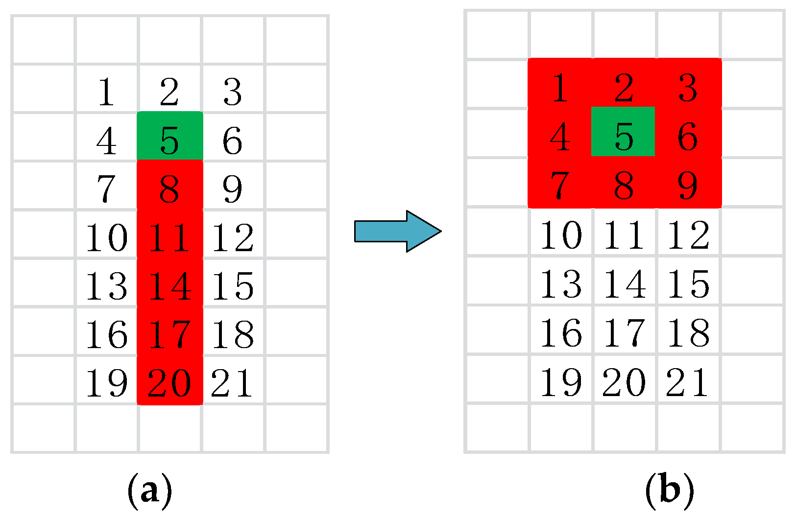
Like Figure 2a, other researchers used a few points in front of the prediction point to predict the coal seam thickness in the marching direction, but this method just considered coal seam data in one direction on the coal seam surface. In order to consider the spatial distribution of coal seams, we chose the structural elements centered on the prediction point on the coal seam surface that is shown in Figure 2b. Due to the missing edge data of structural elements when the center of the structural elements is at the boundary of the known coal seam data, the RBF-Kriging algorithm is used to interpolate the missing data. Like in Figure 3, when the center of the 3 × 3 structural element is the point A, the blue points need to interpolate with the RBF-Kriging algorithm.

3.2. Structural Element Transition Probability

For a 3 × 3 structural element s t = { z 1 , z 2 , , z 9 | z i R + } that contains nine coal seam points z i , and the spatial distribution is mainly composed of one unit distance point and 2 unit distance point in eight directions. Where, one unit distance and 2 unit distance points contain four points, respectively. In the process of iteration prediction in the marching direction, we use the structural elements st i to predict the coal seam thickness in the point i, and predict the next coal seam thickness in turn. The structural element moves in the marching direction with the iteration prediction. Due to the structural elements movement in the prediction process, there is data overlap between two structural elements that move one step and two steps. Figure 4 shows the data overlap diagram of one step moving.
In Figure 4, the point marked “1” indicates the data distribution point in the initial state, and the point labeled “2” indicates the data distribution point under the state of moving one step. The point labeled “1/2” indicates that the data distribution point overlapped by both states.
Due to the interdependencies among structural elements, the structural element of the next state is determined by the structural elements of the current state and previous states. For the Markov chain, the state of the next moment of the system is uniquely determined by the current state and it does not depend on its past [17]. Thus, the transition probabilities that were calculated by the Markov chain are used to measure the influence of these points, which have the equal distance to a prediction point in a structural element, on this prediction point.
For computing the transition probability, we adopt the method of the Markov process [18] that needs to divide the data state that depended on some criterion for computing the transition probability. Assuming that the structural elements S t = { s t i 1 , s t i , s t i + 1 | 1 i n } has interdependencies, the state S = { s 1 , s 2 , , s i , , s m | 1 i m } of each data point in the structural elements is expressed as the state division:
min | h s t i + 1 , j h s t i , j | Δ h max | h s t i + 1 , j h s t i 1 , j | , 1 i n , 1 j 9 ,
where m is the number of state, h s t i , j is the coal seam thickness value at each point in the structural elements, and Δ h is the maximum difference of coal seam thickness within a state. Notice that the rationality of the state division must be maintained for each coal seam thickness data. If the state division is too fine, then each point data is in a separated state. As a result, the calculation amount increases and the minimal changes in the data will cause the chain reaction in the prediction process to not be conducive in maintaining the stability of the model. If the state division is too rough, all of the data in the structure elements is in a single state, and there is no spatial distribution information used in the prediction of the coal seam thickness. Thus, the maximum and minimum values between the two structural elements need to be dynamically recalculated after movement.
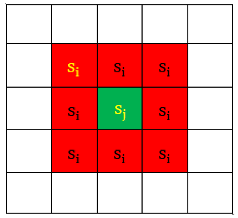
It contains nine points, that is eight controlling points and a prediction point in the center in a structural element, and each point would be divided to a state s. Assuming the state of controlling point is s i and the prediction point is s j , and the each controlling point and prediction point form a state pair, like the two yellow state in the Figure 5, is a state pair. The change from one state pair to other state pair is called state pair transition.
Figure 5 shows the state diagram of the structural element. In Figure 5, there are eight state pairs between the known data and the predicted data, and the yellow marking shows an example of a state pair. Assuming that there are n states and there are n possible state at each point, so the total number of state pairs is n 2 and the number of possible state pair transitions are n 4 . If using the state pairs directly solves the transition probabilities, then the computational complexity is huge. Fortunately, in our application, the state of a prediction point is fixed, i.e., the second state of the state pair is determined. Thus, the transition probability can be obtained by the first state of the state pair. The total state transition number is n 2 . The state transition probability can be calculated, as follows [19]:
P ( S t ) = P { s t i , j 1 = s i | s t i , j = s j } = P s i s j ( m ) { 0 P s i s j ( m ) 1 , s i , s j S i , j S P s i s j ( m ) = 1 , s i , s j S ,
where, P s i s j ( m ) is approximated by the state transition frequency [20] and m represents the number of steps of the structure element movement. In this paper, one-step transition probability is used, and thus, m = 1.
For an individual structural element, state transition probability between pairs of points can describe its spatial characteristics and the effect of equidistance, for which the data input form is shown in Figure 6. For the convenience of data processing in the STTP-GPR algorithm and other compared algorithms, the 3 × 3 structural element is then transformed into vector that expresses the thickness around the prediction points, and it adds the spatial information descripted by transition probability. As we decompose the structural element to the original coal seam thickness and spatial information, and combine the coal seam data and spatial information to predict unknown points, this decomposition method does not affect the prediction results.

3.3. The GP Algorithm

GP is a kind of machine learning method that was developed on the basis of the combination of Bayesian theory and statistical learning theory, which has a greater advantage in dealing with small samples and nonlinear problems. Meanwhile, it has to be able to calculate the confidence level for predicted values, so that the output results have the meaning of probability.
Gaussian process regression belongs to the supervised learning methods. Its training process can better train and learn the training data, and it contains fewer parameters. For the data D = { ( x i , z i ) } i = 1 n , the input vectors are x i R d and the outputs are z i R . In a finite set of data D, f ( x i ) can be a set of random variables, and its joint distribution of arbitrary dimension and finite variables obey the Gaussian distribution. The Gaussian distribution can be expressed by its mean function m ( x ) and covariance function k ( x , x ) . The covariance matrix embodies the intrinsic relation of different data points in the Gaussian process algorithm. The Gaussian process is defined as f ( x ) ~ G P ( m ( x ) , k ( x , x ) ) .
It is assumed that joint distribution of training points X with y and test points x with z is jointly normal under a Gaussian process:
[ z z ] ~ N ( 0 , [ K ( X , X ) + σ n 2 I K ( X , X ) K ( X , X ) K ( X , X ) ] )
where K is the covariance matrix that is created by the chosen kernel function, σ n 2 is the observation noise, and I is the identity matrix. In general, the Gaussian kernel function (RBF) is chosen. The conditional probability p ( z | z ) follows a Gaussian distribution:
z | z ~ N ( K ( X , X ) ( K ( X , X ) + σ n 2 I ) 1 z , K ( X , X )   K ( X , X ) ( K ( X , X ) + σ n 2 I ) 1 K ( X , X ) )
The best estimate for z is the mean of this distribution:
z = K ( X , X ) ( K ( X , X ) + σ n 2 I ) 1 z
The Gaussian process regression algorithm [10] assumes that its prior information distribution satisfies the Gaussian distribution in predicting data, and its probability density among data points depends on the kernel function. The kernel function describes the internal relations of data points in the Gaussian process model. It is usually selected by human experience, which may cause the relations between points to be inaccurate. As a result, it cannot accurately model the spatial distribution of the coal seam.

3.4. Implementation of STTP-GPR

The basic steps of the proposed STTP-GPR algorithm are summarized, as follows:
  • Step 1: acquire the coal seam thickness data, as H = { z 1 , z 2 , , z n | z i R + , 0 < i n } ;
  • Step 2: divide the acquired data into 3 × 3 structural elements S t = { s t i 1 , s t i , s t i + 1 | 1 i n } and the center of each structural element is the prediction point using the method described in Section 3.1;
  • Step 3: the structural elements are divided into training sets and test sets according to the data ratio of 8:2, and attains the distribution of known coal seam thickness;
  • Step 4: divide the state of each point in the structure element according the Formula (12);
  • Step 5: calculate the state transition probability within structural element through the formula is P ( S t ) = P { s t i , j 1 = s i | s t i , j = s j } = P s i s j ( 1 ) ;
  • Step 6: calculate the transition probability between structural elements, and the transition probability is P ( s t i 1 , s t i ) = P { s t ( i 1 ) = s i | s t ( i ) = s j } = P s i s j ( 1 ) ;
  • Step 7: calculate the conditional probability between structural elements, where the conditional probability is P ( s t i | s t i 1 ) = P ( s t i 1 , s t i ) / P ( s t i 1 ) ;
  • Step 8: combine the structural element transition probabilities and joint distribution of known coal seam thickness to derive a posterior probability distribution of prediction model z = S T T P _ G P ( m ( s t ) , P ( s t i | s t i 1 ) ) , that uses the structural element transition probabilities to replace the covariance function in GP algorithm. where z represents predicted coal seam thickness value, and m ( s t ) represents the mean value of structural elements; and,
  • Step 9: predict the coal seam thickness at different positions.
Especially, the structural elements contain nine coal seam points that each point belongs to a certain state, and z is a coal seam point value that is computed through z = S T T P _ G P ( m ( s t ) , P ( s t i | s t i 1 ) ) , which uses the structural element transition probabilities to replace the covariance function in GP algorithm.
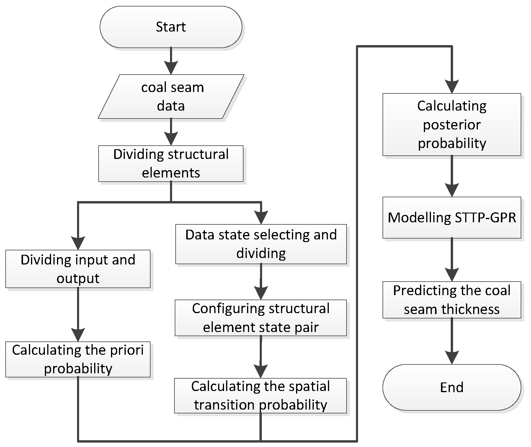
Figure 7 shows the flow chart of the proposed STTP-GPR algorithm.

4. Experimental Results and Analysis

4.1. Coal Seam Forecasting Based on Simulated Data

In view of the complexity of the coal rock interface, the coal seam is normally modelled as the double cosine surface [21]:
Z = 2.4 + 0.2 × sin ( π × w 100 ) 0.2 × sin ( π × l 100 ) .
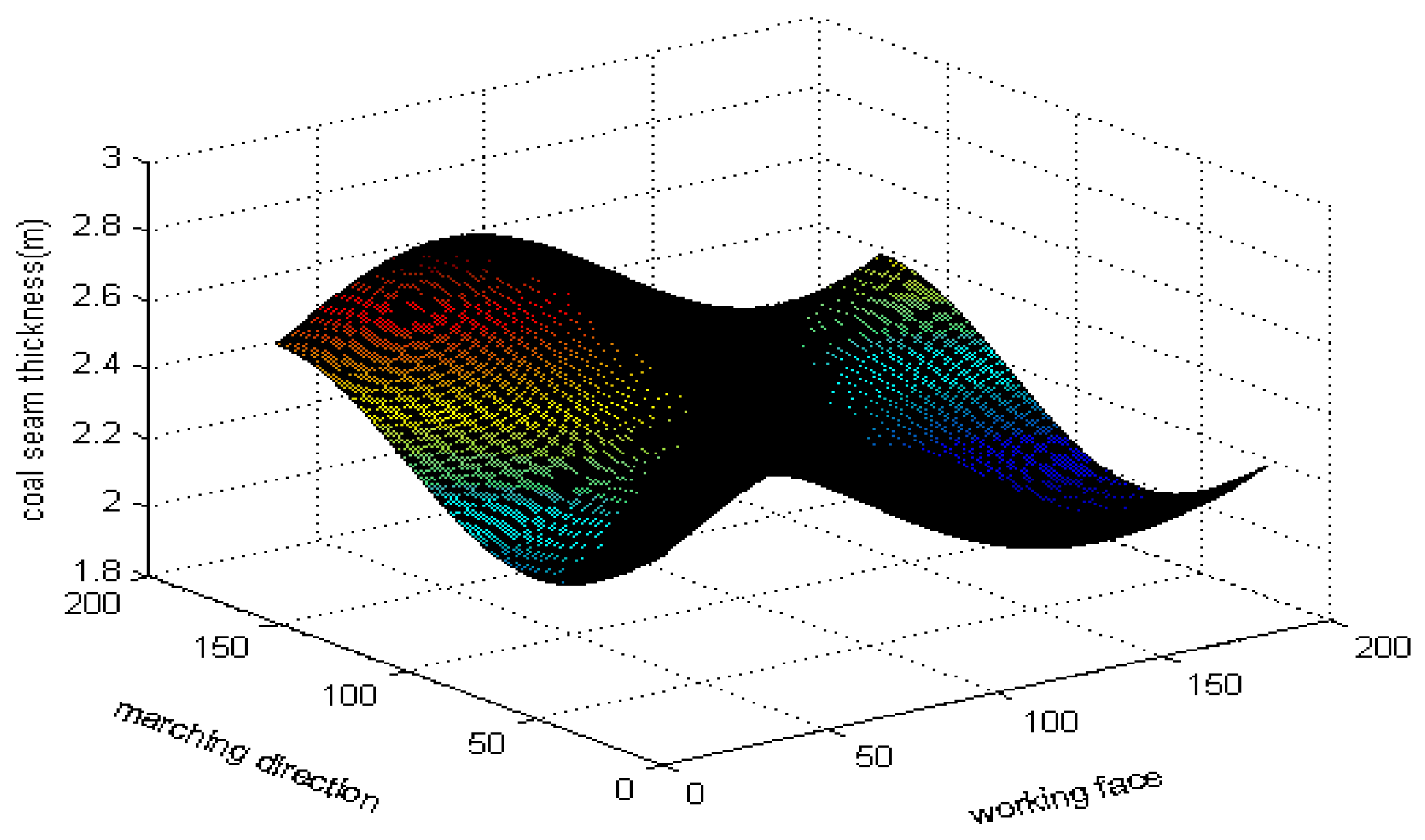
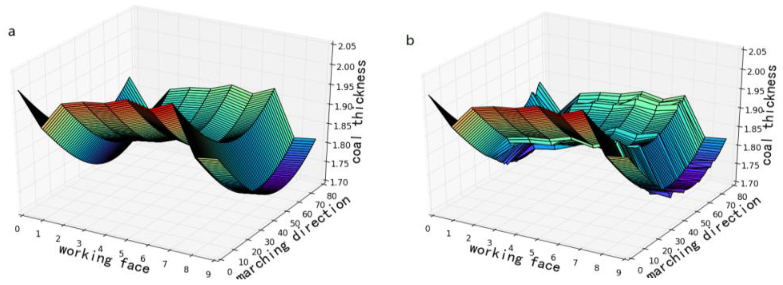
Figure 8 shows the simulated surface. In this experiment, 30 sets of continuous data were randomly generated from the simulated surface as a training set and a test set. The average mining height was set to be 2.4 m.
In order to ensure the integrity of the structural elements in the moving process, the data at the edge of the coal-rock interface is gradually processed by RBF-Kriging interpolation.
The coal seam data was then normalized to [0,1]:
z ¯ ( x i ) = z ( x i ) m i n ( z ( x ) ) max ( z ( x ) ) m i n ( z ( x ) )
where z ( x ) is the original data, m i n ( z ( x ) ) and max ( z ( x ) ) are the maximum and minimum values of z ( x ) respectively, z ¯ ( x i ) are the normalized data. For the transition probabilities, no normalization operations were carried out, since they are in the range of [0,1]. The normalization operation can improve the speed and convergence of subsequent data prediction.
Figure 9 shows the prediction results in 95% confidence interval obtained using the proposed STTP-GPR algorithm.
From Figure 9, it can be seen that the trends of prediction data matches the real data very well. Overall, the maximum prediction error is less than 0.03 m and the average absolute error remains around 0.02 m. From Figure 8, it can be seen that the proposed STTP-GPR algorithm has a good performance in dealing with the locality change problem, which verifies that the spatial distribution of the coal seam that is near the prediction point plays an irreplaceable role in the prediction process. Processing the structural distribution of coal seams correctly is the key to improving the prediction accuracy of coal seams, and by expressing the structural distribution through transfer probabilities in local regions. Figure 10 shows the 3D visualization of the real surface and the prediction surface.

4.2. Coal Seam Forecasting Based on Real Data

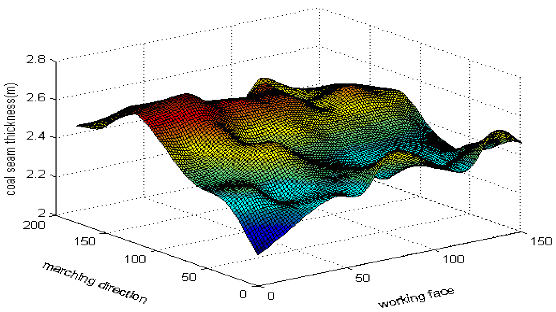
In this experiment, the real data of a thin coal seam face from a coal mine in northern Shaanxi Province of China is used. The real data is interpolated by the proposed RBF-Kriging method for satisfying the structural element integrity. Figure 11 shows the interpolated surface. The sample point interval in working surfaces is 1.5 m and the depth-web is 0.8 m. The total number of sample points for each cutting is 10. For the coal seam data, the training sample pairs are obtained while using the data preprocessing method that is described in Section 3.1, in which each pair of sample contains one structural element with eight points and one output corresponds to it.
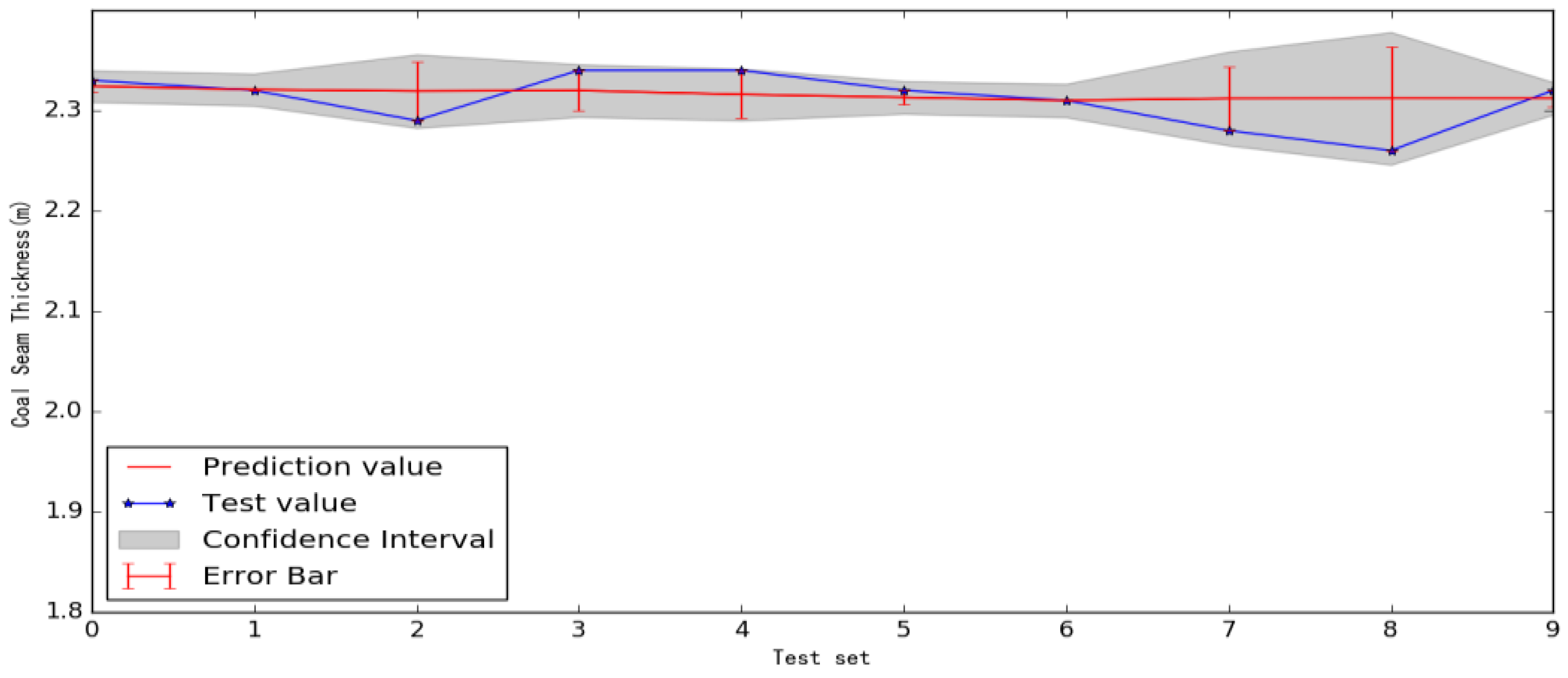
30 pairs of real data are selected in this experiment, of which 20 data pairs are used as the training data and 10 data pairs are used as test data. Figure 12 presents the prediction results using the proposed STTP-GPR algorithm.
The absolute average error in the test set remains around 0.025. The prediction error at the third point and the last two points of the test set is relatively high, due to the coal seams being mutational at these points. Analysis of the prediction error on all test sets shows that the overall prediction error is less than 0.031. From Figure 12, it can be seen that the prediction value of STTP-GPR algorithm at second data and the last three data in the test set has larger error, but their error is less than 0.03 by taking into account the spatial structure information and the maximum error in test set is less than the error that is predicted by GPR algorithm, as depicted in Section 4.3. From the real coal seam data, it can be seen that the frequency of local fluctuations in the coal seam during its evolution is relatively large; in the proposed STTP-GPR algorithm, the transition probability is mainly divided by human experience in the calculation process, resulting in the inaccurate division of the interval or a failure to describe the structure information. In the future, we will focus on the study of how to accurately express the local spatial structure information of the coal seam and the relationship between the local spatial structure information and the global spatial structure information.
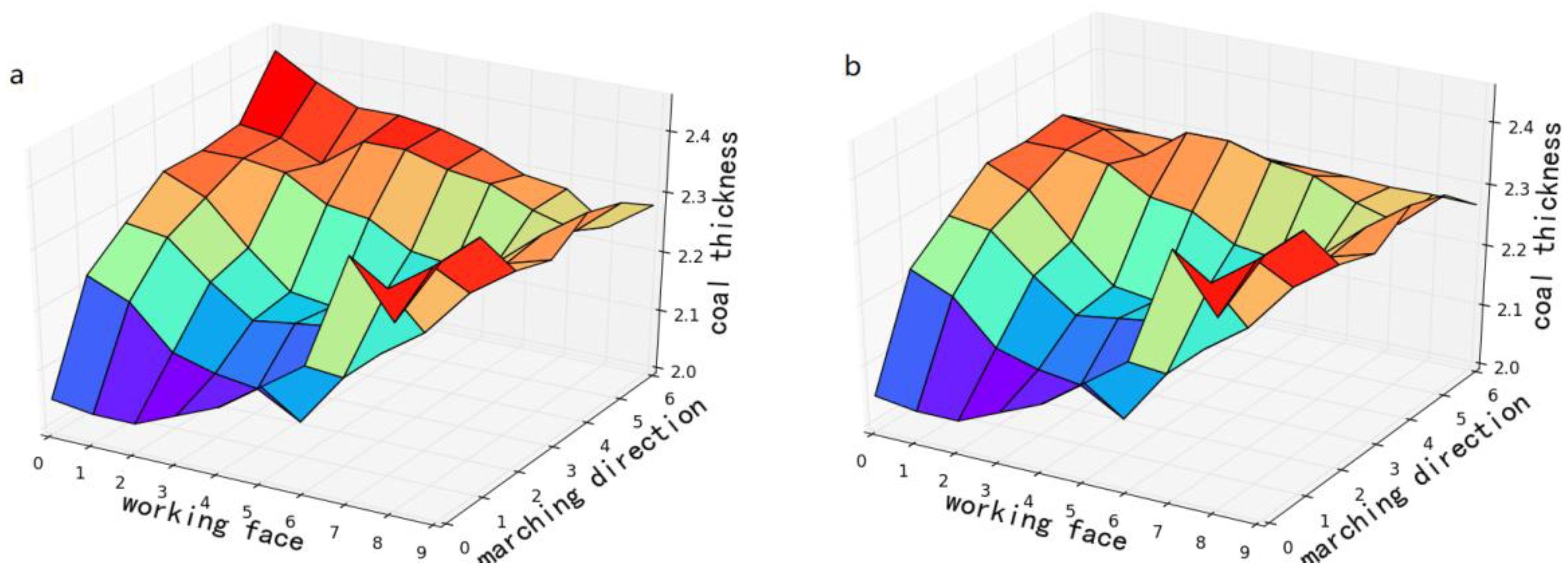
Figure 13 shows the real surface and predicted surface in order to visually represent the pros and cons of the prediction algorithm in the coal-rock interface identification process while using the real data. The predicted surface shown in Figure 13 is the upper surface of the coal seam is obtained from the predicting and known data. The real surface is obtained from the known data in the test set. It can be seen that the predicted surface can accurately express coal seam movements and changes in coal seam thickness, especially in the local district.

4.3. Performance Comparison with the Existing Methods

Due to predicting the coal seam thickness through the proposed STTP-GPR algorithm with data filling at the edge of structural elements moving interpolated by the proposed RBF-Kriging algorithm, we compare our predicting algorithm with the BP neural network (BPNNs) algorithm, SVR algorithm, GPR algorithm [8,22] in this Section, and BPNNS, SVR, and GPR still predict the coal seam thickness without transition probability and interpolated data. A 5-6-8-1 four-layer BP neural network was constructed. The SVR algorithm uses the Gaussian kernel function as the data mapping method to predict the training set data. The Mean Absolute Error (MAE) was used to measure the performance of the four algorithms in prediction of the coal seam thickness. The above real coal seam data of 30 training sets was used in this experiment.
Table 1 shows the average absolute error that was predicted by using the four prediction algorithms. From Table 1, it can be seen that the proposed STTP-GPR algorithm is superior to the other algorithms. The prediction value of the SVR algorithm changes with the change of kernel function, and the kernel function usually depends on empirical selection. The neural network algorithm may over fit in processing small sample data, and because of a lack of sample data, the prediction error is usually worse. The proposed STTP-GPR algorithm that includes the local spatial attributes highlights the influencing factors of local data for unknown data, and the predicted values have little difference with the actual coal seam data, which reflects the changing trend of coal seams. At the same time, it enhances the ability within a certain error range for the local prediction lag that is caused by the coal seam geology change.

5. Conclusions

A STTP-GPR coal seam prediction algorithm with the cutting data being interpolated by the RBF-Kriging is proposed. The RBF-Kriging interpolation algorithm ensures the data integrity of the structural elements at the edge of the marching direction. It uses the transition probabilities between the structural elements to represent the spatial distribution structure. By taking into account the spatial distribution of coal seams, the proposed method makes up for the deficiencies only using the marching direction to predict the coal seam without considering the influence in other directions, thus improving prediction performance. The proposed method is verified using the simulated and real coal seam data. The experimental results show that the prediction accuracy of the proposed STTP-GPR algorithm is superior in comparison to the popular BP neural network, SVR algorithm, and GPR algorithm.
In practical application, due to the precise prediction of coal–rock interface and coal seam thickness of next cutting, the proposed method enables the shearer to automatically track the coal-rock interface in mining and adjust the coal cutting height to improve the production efficiency and coal quality. The proposed method can be used both for manually operated shearers and for computer controlled shearers.

Author Contributions

Conceptualization, W.K. and A.Q.; Methodology, W.K.; Software, W.K.; Validation, A.Q., W.K. and H.L.; Formal Analysis, W.K.; Investigation, H.L.; Resources, A.Q.; Data Curation, A.Q. and W.K.; Writing-Original Draft Preparation, W.K.; Writing-Review & Editing, G.Z.; Visualization, W.K.; Supervision, A.Q.; Project Administration, W.K.; Funding Acquisition, A.Q.

Funding

This research was funded by National Natural Science Foundation of China (No. 61674121).

Conflicts of Interest

The authors declare no conflict of interest.

References

  1. Yuan, L.; Zhang, N.; Kan, J.G.; Wang, Y. The concept, model and reserve forecast of green coal resources in China. J. China Univ. Min. Technol. 2018, 47, 1–8. [Google Scholar]
  2. Chen, D. Discussion on the technology and development direction of coal mine safety in China. Sci. Technol. Inf. 2013, 9, 150. [Google Scholar]
  3. Zhao, T.; Liu, C. Roof instability characteristics and pre-grouting of the roof caving zone in residual coal mining. J. Geophys. Eng. 2017, 14, 1463–1474. [Google Scholar] [CrossRef] [Green Version]
  4. Xiao, M.; Zhang, G.; Breitkopf, P.; Villon, P.; Zhang, W. Extended Co-Kriging interpolation method based on multi-fidelity data. Appl. Math. Comput. 2018, 323, 120–131. [Google Scholar] [CrossRef]
  5. Wu, W.; Yang, Y.; Chen, Y. Kriging Interpolation Method Optimized by LSSVM and Its Application in Predicting Coal Thickness. Coal Technol. 2015, 34, 89–91. [Google Scholar]
  6. Qiao, G.; Cai, H.; Zhou, A.; Yang, F.; Wang, H.; Jing, Y.; Yang, L.; Ma, L. Coal Quality Prediction Model of Drilling Coal Based on Kriging Interpolation Method. Coal Technol. 2016, 35, 151–153. [Google Scholar]
  7. Li, Y.M.; Liu, E.M.; Xue, G.H.; Miao, W. Coal-Rock Interface Identification Method Based on Dimensionless Parameters and Support Vector Machine. Appl. Mech. Mater. 2015, 716–717, 843–847. [Google Scholar] [CrossRef]
  8. Wang, B.; Liu, S.; Huang, L. Comprehensive forecast system of the thickness of coal seam and its application. In Proceedings of the International Conference on Mechatronic Science, Jilin, China, 19–22 August 2011. [Google Scholar]
  9. Mair, S.; Brefeld, U. Distributed robust Gaussian Process regression. Knowl. Inf. Syst. 2017, 55, 415–435. [Google Scholar] [CrossRef]
  10. Richardson, R.R.; Osborne, M.A.; Howey, D.A. Gaussian process regression for forecasting battery state of health. J. Power Sources 2017, 357, 209–219. [Google Scholar] [CrossRef]
  11. Marcotte, D.; David, M. Trend surface analysis as a special case of IRF-k, kriging. Math. Geol. 1988, 20, 821–824. [Google Scholar] [CrossRef]
  12. Ghiasi, Y.; Nafisi, V. Strain estimation using ordinary Kriging interpolation. Surv. Rev. 2016, 48, 361–366. [Google Scholar] [CrossRef]
  13. Klauberg, C.; Hudak, A.T.; Bright, B.C.; Boschetti, L.; Dickinson, M.B.; Kremens, R.L.; Silva, C.A. Use of ordinary kriging and Gaussian conditional simulation to interpolate airborne fire radiative energy density estimates. Int. J. Wildland Fire 2018, 27, 228–240. [Google Scholar] [CrossRef]
  14. Mukhtar, A.; Ching, N.K.; Yusoff, M.Z. Optimal Design of Opening Ventilation Shaft by Kriging Metamodel Assisted Multi-objective Genetic Algorithm. Int. J. Model. Optim. 2017, 7, 92–97. [Google Scholar] [CrossRef]
  15. Li, W.; Luo, C.; Yang, H.; Fan, Q. Memory cutting of adjacent coal seams based on a hidden Markov model. Arab. J. Geosci. 2014, 7, 5051–5060. [Google Scholar] [CrossRef]
  16. Fianu, S.; Davis, L.B. A Markov Decision Process Model for Equitable Distribution of Supplies under Uncertainty. Eur. J. Oper. Res. 2017, 264, 1101–1115. [Google Scholar] [CrossRef]
  17. Amsalu, S.B.; Homaifar, A.; Esterline, A. A Simplified Matrix Formulation for Sensitivity Analysis of Hidden Markov Models. Algorithms 2017, 10, 97. [Google Scholar] [CrossRef]
  18. Eidsvik, J.; Mukerji, T.; Switzer, P. Estimation of Geological Attributes from a Well Log: An Application of Hidden Markov Chains. Math. Geol. 2004, 36, 379–397. [Google Scholar] [CrossRef]
  19. Larsen, A.L.; Ulvmoen, M.; Omre, H.; Buland, A. Bayesian lithology/fluid prediction and simulation on the basis of a Markov-chain prior model. Geophysics 2006, 71, R69–R78. [Google Scholar] [CrossRef]
  20. Li, J.; Qu, Y.; Li, C.; Xie, Y.; Wu, Y.; Fan, J. Learning local Gaussian process regression for image super-resolution. Neurocomputing 2015, 154, 284–295. [Google Scholar] [CrossRef]
  21. Min, Z.; He, Y. Research on Prediction of Coal and Rock Based on Grey Neural Network. Autom. Instrum. 2012, 2, 16–18. [Google Scholar]
  22. Youkuo, C.; Yongguo, Y.; Wangwen, W. Coal seam thickness prediction based on least squares support vector machines and kriging method. Electron. J. Geotech. Eng. 2015, 20, 167–176. [Google Scholar]
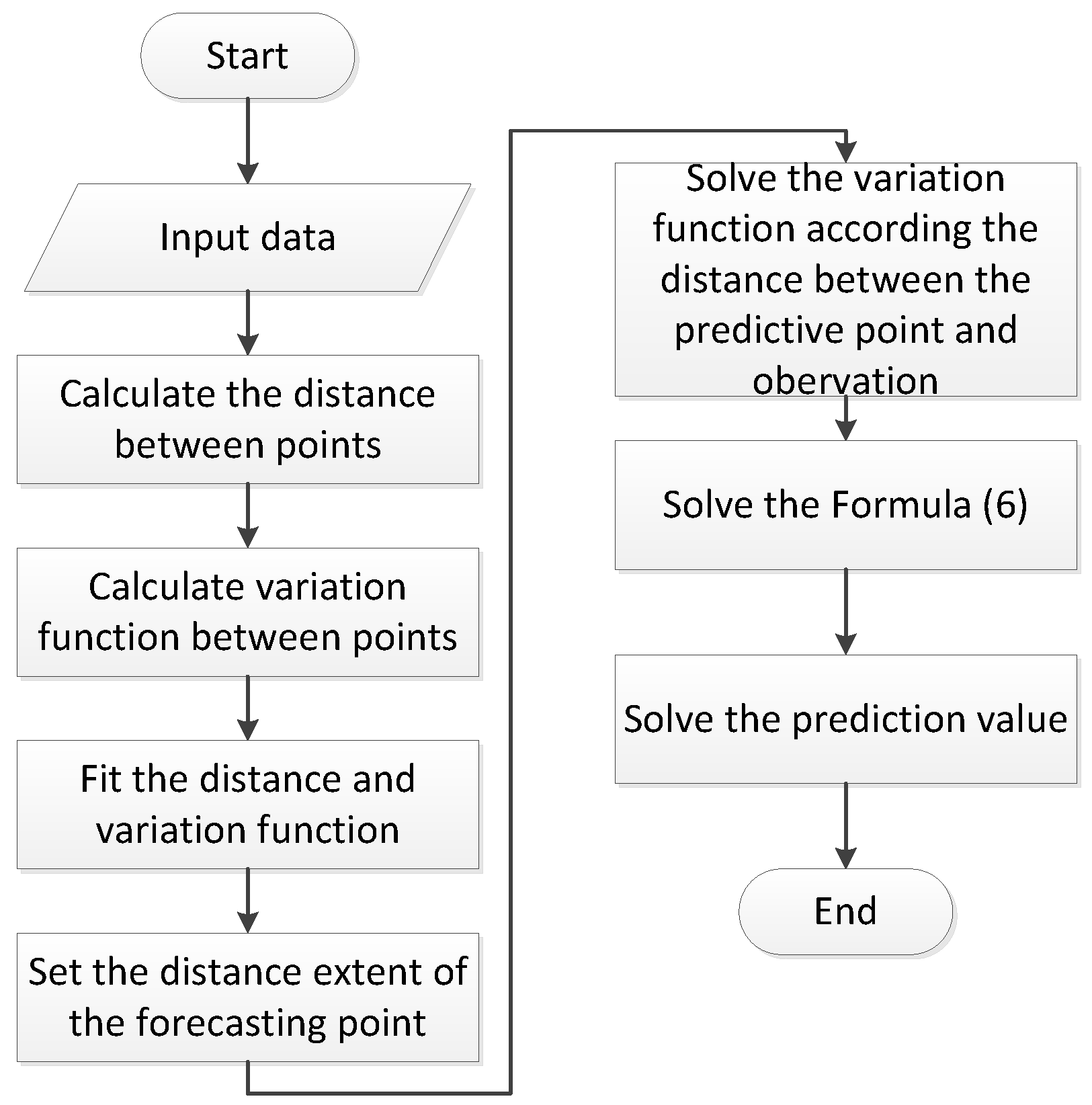
Figure 1. Flowchart of the proposed RBF-Kriging interpolation algorithm.
Applsci 09 01144 g001
Figure 2. Change of prediction mode diagram, (a) is the prediction mode in the marching direction, (b) is our prediction mode through structural elements. It used the red color data to predict the green unknown data.
Applsci 09 01144 g002
Figure 3. Radial Basis Function (RBF-Kriging) algorithm interpolated diagram (blue points).
Applsci 09 01144 g003
Figure 4. Diagram of overlapping with structural elements movement.
Applsci 09 01144 g004
Figure 5. Diagram of structural elements state.
Applsci 09 01144 g005
Figure 6. Form of data transformation.
Applsci 09 01144 g006
Figure 7. Flowchart of structural element transition probability based Gaussian process progression (STTP-GPR).
Applsci 09 01144 g007
Figure 8. Simulated coal seam surface.
Applsci 09 01144 g008
Figure 9. Test-Prediction Data Graph of improved algorithm.
Applsci 09 01144 g009
Figure 10. Three-dimensional (3D) visualization of the coal seam surface obtained from the simulated experiment: (a) real surface and (b) prediction surface.
Applsci 09 01144 g010
Figure 11. Interpolated surface from the real coal seam data
Applsci 09 01144 g011
Figure 12. Prediction results obtained by using the proposed STTP-GPR algorithm and real coal seam data.
Applsci 09 01144 g012
Figure 13. 3D visualization of the coal seam surface obtained from the real experiment: (a) Real surface and (b) prediction surface.
Applsci 09 01144 g013
Table 1. Mean absolute error.
AlgorithmMAE(m)
SVR0.061
BPNNs0.043
GPR0.036
STTP-GPR0.025