Collinear Deflection Method for the Measurement of Thermal Conductivity of Transparent Single Layer Anisotropic Material

Abstract

Transparent anisotropic materials have garnered attention along with the growth of the semiconductor and display industries. Transparent anisotropic materials have the characteristic of varying electrical, optical, and thermal properties based on their crystal orientation, and many studies are being conducted on this topic. In order to utilize transparent anisotropic materials properly, thermal properties such as thermal conductivity are essentially required. However, due to the limitations of the existing thermal property measurement methods for transparent anisotropic materials, it is difficult to provide the thermal properties of transparent anisotropic materials. To address this problem, a transparent anisotropic collinear method capable of measuring the effective thermal conductivity of a transparent anisotropic material according to its crystal orientation is proposed in this paper. To this end, the internal temperature distribution of a transparent anisotropic material and the phase delay of the probe beam were theoretically derived through a numerical analysis model that uses a three-dimensional heat conduction equation. This model was applied to anisotropic thermal conductivity with orthorhombic structure. To verify the proposed method of measuring the thermal conductivity of a transparent anisotropic material, the thermal properties of 3 mm-thick A-plane sapphire glass were measured and compared with those of the existing literature. It was confirmed that the absolute errors were less than about 4 W/mk.

1. Introduction

As the display industry grows and transparent flexible displays attract attention, studies on new materials used in transparent flexible substrates and transparent electrodes continue to actively be conducted [1,2,3,4]. In particular, many studies have been conducted on transparent anisotropic materials whose properties, such as the electrical conductivity, light transmittance, and thermal conductivity, vary depending on their crystal orientations [5,6,7]. However, materials with high flexibility and high light transmittance generally have wide gaps between molecules, which leads to low thermal conductivity [8]. Moreover, in the case of transparent anisotropic materials formed using composite materials, they can be applied to systems only when their accurate thermal properties in the applied direction are known because those properties are significantly different depending on the direction. Therefore, for the optimal thermal design of displays that use such new transparent anisotropic materials, accurate information on the thermal properties of the materials is required. Due to the limitations of the existing thermal property measurement methods for transparent anisotropic materials [9,10,11,12,13,14,15,16,17], the need for developing new measurement methods is increasing.

When a heat source is applied to a material, its temperature change essentially depends on its thermal properties. Therefore, the thermal properties of a material can be determined by measuring its temperature change, and there are various methods to do so. The categories of thermal property measurement methods can be divided according to the contact or non-contact of the temperature change measuring sensor.

Table 1. Various thermal property measurement methods and limitations.

	Method	Limitation
Contact	DC heating [9,10,11]	Conductive materials only
	Pulse heating [12,13,14]	Conductive materials only
	Laser calorimetry [15]	Large amount of heat loss
	3ω method	Complexity damage of specimen
Non-Contact	Photo Acoustic [15]	Low accuracy
	Laser Flash [17]	Damage of specimen & Limitation of shape/size
	Photothermal radiometry [15]	Problem of emissivity factor
	Photothermal reflection [15]	Standardization of roughness on surface of specimen
	Photothermal displacement [15]	Surface treatment of specimen
	Photothermal deflection [15]	Increase of S/N

summarizes various measurement methods [9,10,11,12,13,14,15,16,17] and their limitations.

Thermal property measurement using the photothermal effect is attracting attention as one of the non-contact methods with high accuracy. Among the photothermal thermal property measurement methods, the photothermal deflection method is currently the most actively researched and it has universal applicability to various materials as well as high accuracy [18,19,20,21,22,23,24,25,26,27,28,29,30]. The photothermal deflection method must be applied differently depending on the material. Therefore, developing specialized photothermal deflection methods is a key issue.

The photothermal deflection method uses two types of lasers—pump beam and probe beam—for measurement, and can be classified as either a mirage deflection method [18,19,21,22,23,26,27,28,29] or a collinear deflection method [20,24,25,30] depending on the alignment of the two lasers, as shown in Figure 1. The mirage deflection method is mainly applied to optically thick materials, while the collinear deflection method is applied to transparent or optically thin materials.

In the case of the mirage deflection method, the measurement method for single layer isotropic materials has been established by researchers, including Jackson [18], Salazar [21,27], and Bertolotti [22,26], and the measurement method for single layer anisotropic materials has been established by Jeon et al. [29]. In the case of the collinear deflection method, studies limited to isotropic single/double layer materials were conducted by Jonathan et al. [20,24] and Salaszar et al. [25,30]. Very restricted studies on the photothermal deflection method for anisotropic materials have been conducted by Iravani et al. [31], Quelin et al. [32], and Salazar et al. [33,34].

Iravani et al. [31] analyzed three-dimensional (3D) heat conduction equations for semi-infinite solid and slab models to describe the propagation of heat waves in anisotropic materials. Quelin et al. [32] analyzed the heat conduction equation for 3D models by applying the thermal conductivity with only the component in the principal axis direction to poly (4-BCMU). Based on this, they proposed a relation for the mirage deflection method and showed that the results were in relatively good agreement with the measured experimental data. Salazar et al. [33,34] proposed a 3D analysis model for the case where only the thermal conductivity component in the principal axis direction was present based on the mirage deflection method and conducted research on the determination of the thermal diffusivity using the relationship of the anisotropic properties of the thermal conductivity. Through their research, they showed that the analysis method applied to isotropic materials could also be applied to anisotropic materials. In summary, the previous studies on the photothermal deflection method [18,19,20,21,22,23,24,25,26,27,28,29,30,31,32,33,34] were conducted only for the mirage deflection method, which measures the thermal properties of optically thick isotropic/anisotropic materials, but not for the collinear deflection method, which measures the thermal properties of transparent anisotropic materials.

Therefore, this study investigates the collinear deflection method for measuring the thermal conductivity of a transparent anisotropic material depending on its crystal orientation. To this end, the temperature distribution of a single layer transparent anisotropic material was derived through numerical analysis using a 3D heat conduction equation. To measure the thermal conductivity of the transparent anisotropic material using the derived temperature distribution, the deflection of the probe beam was analyzed. To verify this, measurement was performed for the 3 mm-thick A-plane sapphire glass whose thermal conductivity in the principal axis direction was well known, and it was found that the effective thermal conductivity ($k_{eff}$) could be derived according to the measurement direction ($\theta$, $k_{\theta =0°}=k_{11}$, $k_{\theta =90°}=k_{22}$).

2. Background Theory and Method

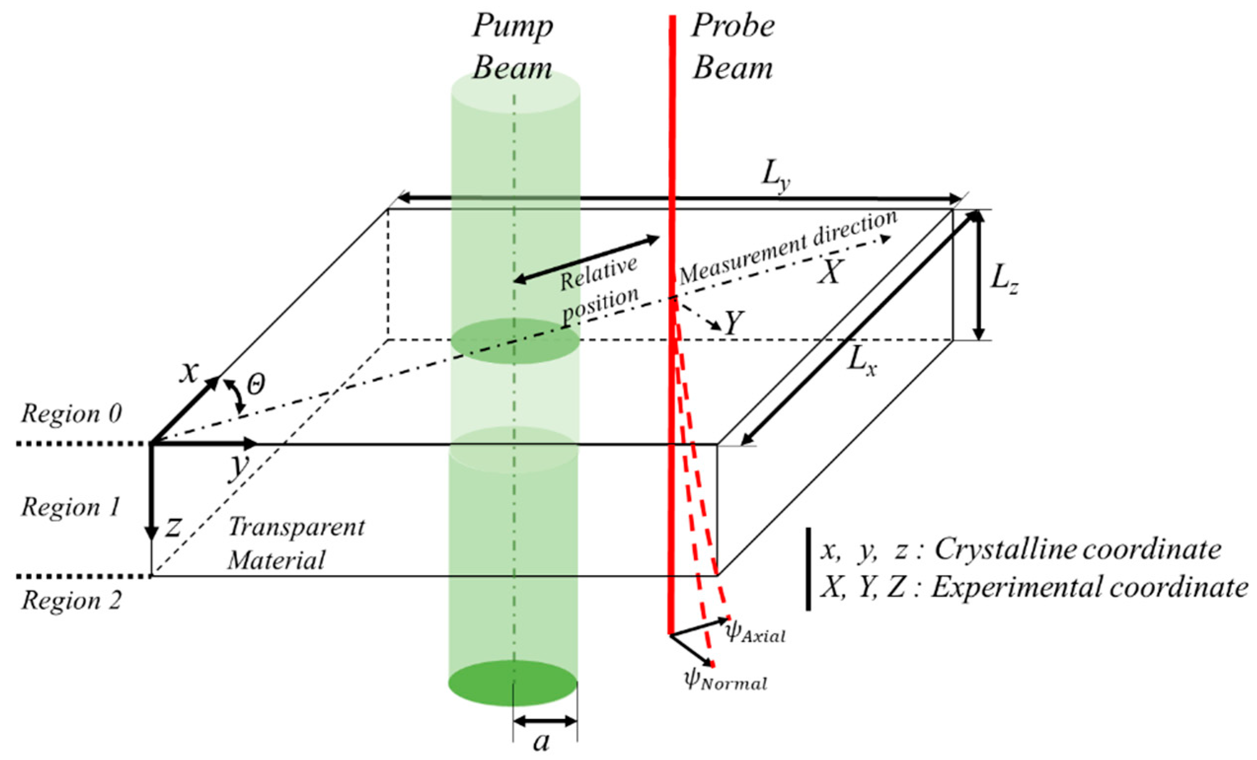
2.1. Collinear Deflection Method

The photothermal effect used in this study is a phenomenon in which heat is generated as the energy level of a material increases due to the photons colliding with the surface of the material [15,35]. The collinear deflection method uses the temperature gradient inside the material, which is induced from the photothermal effect by the modulated laser (pump beam). This temperature gradient causes changes in the density of the transparent material, which leads to changes in the refractive index of the material. As shown in Figure 1b, when the probe beam is irradiated on the area where temperature and refractive index gradients occurred so it is perpendicular to the specimen and parallel to the pump beam, deflection occurs. In this instance, the deflection angle of the probe beam ($\psi$) can be expressed by Equation (1) [13].

$$\psi ={\displaystyle {\int }_{path}\frac{1}{n}\left(\frac{\partial n}{\partial T}\right){\nabla }_{n}T(x,y,z,t)ds}$$

(1)

where $n$ is the refractive index, $\partial n/\partial T$ is the temperature coefficient of the refractive index, and ${\nabla }_{n}T$ is the temperature gradient perpendicular to the probe beam path.

As a pump beam modulated with a constant period is used, the temperature gradient inside the material also repeats rising (heating) and falling (cooling) according to the heating period of the pump beam. In this case, a time difference occurs between the temperature gradient and pump beam periods depending on the thermal properties of the target material. As a result, when the deflection of the probe beam passing through the temperature gradient is compared with the period of the pump beam, a time difference occurs, as shown in Figure 2, and this is referred to as the phase delay. The phase delay increases as the relative position between the pump beam and probe beam increases, and it varies depending on the thermal properties of the material. Therefore, it is possible to derive the thermal conductivity by analyzing the phase delay according to the relative position.

2.2. Temperature Distribution Analysis

To derive the thermal conductivity by analyzing the phase delay, it is essential to compare the results of the probe beam deflection analysis based on the theoretical temperature analysis with the experiment results.

For the temperature distribution analysis, a 3D single layer solid model with infinite lengths in the $x$ and $y$ directions and finite length in the $z$ direction was selected, as shown in Figure 3. Regions 0 and 2 are air layers surrounding the measurement material (specimen) and Region 1 is the measurement specimen. As the temperature increase by the pump beam is very small and occurs in local areas, only conduction heat transfer was considered in this study. Therefore, the governing equation can be expressed by Equation (2) below.

$$\nabla \cdot \left\{\overrightarrow{k_k}\times \nabla T_k\right\}-{\rho }_k{c}_{p,}{}_k\frac{\partial T_k}{\partial t}=Q_i\begin{array}{cc}\begin{array}{cc}& \end{array}& \end{array}(k=0,1,2)$$

(2)

$$\overrightarrow{k_1}=\left(\begin{array}{ccc}{k}_{1,11}& k_{1,12}& k_{1,13}\\ k_{1,21}& k_{1,22}& k_{1,23}\\ k_{1,31}& k_{1,32}& k_{1,33}\end{array}\right),\begin{array}{cc}& \end{array}{k}_{1,ij}>0\begin{array}{ccc},k_{1,ij}=0(i\ne j),& & \end{array}(i,j=1,2,3)$$

(3)

where $\mathrm{T}$ is the temperature, $k$ is the thermal conductivity, $\rho$ is the density, $C_p$ is the specific heat, and $Q$ is the heat source by the pump beam. The values $k$, $\rho$, and $C_p$ are thermal properties of the object of the measurement and thermal properties of the air layer.

As the target material was thermally anisotropic, the thermal conductivity could be expressed in orthorhombic form, as shown in Equation (3), and an orthorhombic system composed of $k_{1,11}$, $k_{1,22}$, and $k_{1,33}$ components without ${k_{1,ij}|}_{i\ne j}$ components was considered.

As mentioned above, only conduction was considered in this study. Therefore, the boundary conditions can be expressed by Equation (4) below.

$$\begin{array}{l}{T}_0(x,y,0)=T_1(x,y,0)\begin{array}{cccc}& & & \end{array}{q}_0(x,y,0)=q_1(x,y,0)\\ T_1(x,y,L)=T_2(x,y,L)\begin{array}{cccc}& & & \end{array}{q}_1(x,y,L)=q_2(x,y,L)\\ \begin{array}{cccc}& & & \end{array}{q}_1=-\left(k_{1,11}\frac{\partial T}{\partial x}+k_{1,22}\frac{\partial T}{\partial y}{k}_{1,33}\frac{\partial T}{\partial z}\right)\\ \begin{array}{cccc}& & & \end{array}{q}_k=-k_k\frac{\partial T}{\partial x}\begin{array}{cccc}& & & \end{array}(k=0,2)\end{array}$$

(4)

The pump beam is a laser with Gaussian distribution and can be expressed as shown in Equation (5) according to the modulation frequency ($f$), radius ($a$, $1/e^2$ of maximum intensity), and light absorption coefficient of the material ($\lambda$). The pump beam reaches the material through the air layer. As the light absorption coefficient of the air layer is very small and the pump beam is absorbed only by the material, the heat source of the air layer can be expressed as shown in Equation (6). $P_1$ is the intensity of the laser that finally reaches the material and can be expressed by Equation (7) using the initial intensity of the laser ($P_0$) and the reflectivity of the specimen (${\epsilon }_1$).

$$Q_1(x,y,z,t)=-{\lambda }_1\frac{P_1}{4\pi a^2}{e}^{-{\lambda }_{1}z}{e}^{-(x^2+y^2)/a^2}\left[1+\cos (\omega t)\right]$$

(5)

$$Q_k(x,y,z,0)=0\begin{array}{cccc}& & & \end{array}(k=0,2)$$

(6)

$$P_1=P_0\times (1-{\epsilon }_1)$$

(7)

The heat source $Q_1$ consists of a time-independent term and a time-dependent term with a constant period. Only the time-dependent term was considered because the time-independent term does not affect the phase delay. Therefore, the governing equation is a 3D unsteady-state heat conduction equation in which a periodic heat source exists over time. It can be converted into a form in which steady-state analysis is possible by applying a complex transformation method, as shown in Equation (8).

$$\begin{array}{l}{k}_{11}\frac{{\partial }^2{\tilde{T}}_1}{\partial x^2}+k_{22}\frac{{\partial }^2{\tilde{T}}_1}{\partial y^2}+k_{33}\frac{{\partial }^2{\tilde{T}}_1}{\partial z^2}+(k_{12}+k_{21})\frac{{\partial }^2{\tilde{T}}_1}{\partial x\partial y}+(k_{13}+k_{31})\frac{{\partial }^2{\tilde{T}}_1}{\partial x\partial z}+\left(k_{23}+k_{32}\right)\frac{{\partial }^2{\tilde{T}}_1}{\partial y\partial z}\hfill \\ \hfill =i\omega {\rho }_1{c}_{p,1}{\tilde{T}}_1-\frac{P_1}{4\pi a^2}{e}^{-\lambda z}{e}^{-(x^2+y^2)/a^2}\\ \frac{{\partial }^2{\tilde{T}}_k}{\partial x^2}+\frac{{\partial }^2{\tilde{T}}_k}{\partial y^2}+\frac{{\partial }^2{\tilde{T}}_k}{\partial z^2}=i\omega \frac{{\rho }_k{c}_{p,k}}{k_k}{\tilde{T}}_k\begin{array}{cc}& \end{array}(k=0,2)\hfill \\ T_k(x,y,z,t)={\tilde{T}}_k(x,y,z)e^{i\omega t}\hfill \end{array}$$

(8)

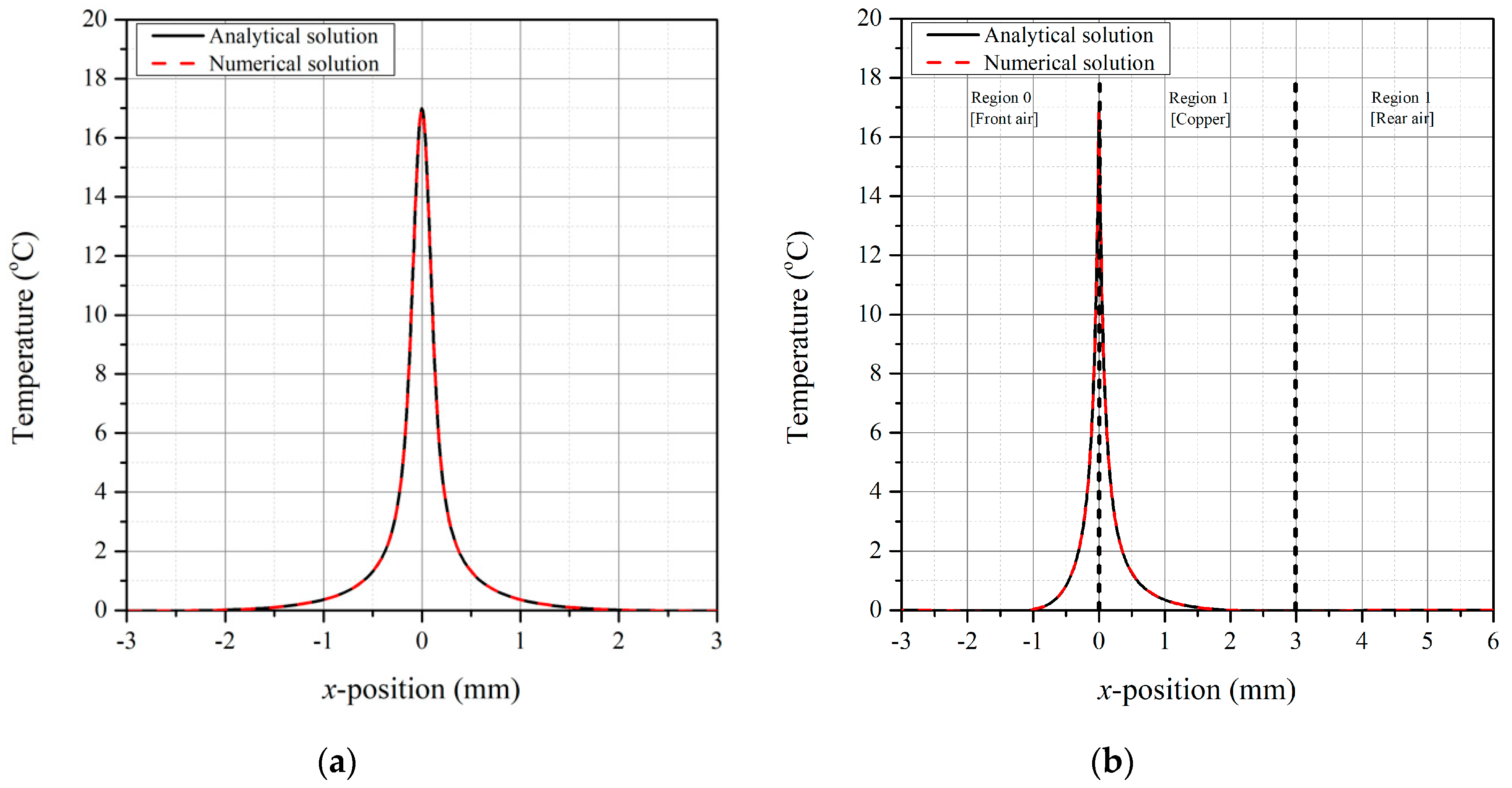
2.3. Numerical Investigation

Based on Equation (8), the temperature distribution was analyzed using COMSOL Multiphysics 5.2a, which is a commercial numerical analysis software program. The governing equation and boundary conditions were applied as explained in Equations (2)–(8). Geometry was constructed using the values shown in

Table 2. Geometry setup for numerical investigation and validation.

		Length (mm)
$L_x$		20
$L_y$		20
$L_z$	Region 0	6
	Region 1	3
	Region 2	6

. To verify the numerical analysis model, node dependency was evaluated and compared with the analytical solution results of the mirage deflection method performed by Jeon et al. [29,36,37]. The material used for evaluating node dependency and verifying the numerical analysis model was copper. The thermal properties used and pump beam radius are summarized in

Table 3. Thermal properties for validation.

	Copper [38]	Air [3]
Density $(\rho ,kg/m^3)$	8930	1.1614
Specific heat capacity $(c_P,J/(kg\cdot K))$	385	1007
Thermal conductivity $(k,W/(mK))$	398	0.0263
Absorption coefficient $(\lambda ,m^{-1})$	7.01 × 107	-
Thermo-optical coefficient $(\partial n/\partial T,K^{-1})$	2.22	2.55 × 10−5
Pump beam radius $(a,\mu m)$	100

.

Table 4. Node dependency evaluation.

Number of Nodes	Computing Time	Temperature (°C)
		X-Position
		0 mm	0.15 mm	0.3 mm	0.45 mm
26,901	10s	2.5412	2.3569	1.3154	0.8852
87,451	22s	2.6542	2.1516	1.2987	0.8751
203,401	49s	2.7567	2.1159	1.2256	0.9045
348,145	105s	2.8457	2.2548	1.4146	0.8912
549,081	120s	2.7542	2.1987	1.3554	0.8759
815,425	223s	3.0157	2.2247	1.4254	0.8945
976,005	253s	3.2187	2.4194	1.4610	0.9153
1,156,393	379s	3.2235	2.4243	1.4646	0.9192
1,357,741	3,868s	3.2234	2.4245	1.4648	0.9190

shows the results derived through the node dependency evaluation. It was found that the temperature in the $x$-axis direction on the material surface ($y=0, z=0$) according to the relative position converged when the number of the nodes was equal to or higher than approximately 970,000. In this study, approximately 1,150,000 nodes were used for the analysis.

Figure 4 compares the analytical solution results of the mirage deflection method for copper with the results of the numerical analysis model constructed in this study. The temperature change (at $y=0, z=0$) in the $x$-axis direction on the material surface (Figure 4a) and the temperature changes (at $x=0, y=0$) in the air layer and inside the material (Figure 4b) were in good agreement with analytical solution (for temperature distribution) of mirage deflection.

2.4. Deflection Analysis

The thermal conductivity of the transparent anisotropic material, which is the target material of this study, varies depending on the crystal coordinates ($x, y, z$) of the material. As the accurate direction of the principal thermal conductivity of the specimen cannot be found by measurement through experiments, it is necessary to compare and analyze the experimental and analytical results. To this end, the crystal coordinates ($x, y, z$) used for the analysis must be matched to the coordinates of the experimental setup ($X, Y, Z$) using the coordinate transformation equation below [37].

$$\begin{array}{l}x=X\cos \theta +Y\sin \theta \hfill \\ y=Y\cos \theta -X\sin \theta \hfill \\ z=Z\hfill \end{array}$$

(9)

Through this process, the effective thermal conductivity can be derived according to the measurement direction ($\theta$). The theoretical thermal conductivity ($k_{\theta ,eff}$) according to the measurement direction ($\theta$) can be expressed by the principal thermal conductivity and direction cosine, as shown in Equation (9) [39,40,41,42]. $k_{1,11}$, $k_{1,22}$, and $k_{1,33}$ are the principal thermal conductivities for each axis, and $l, m, \mathrm{and} n$ are the direction cosines for the $x, y, \mathrm{and} z$ axes, which are the crystal coordinates of the material, respectively.

$$\begin{array}{l}{k}_{1,11}{x}^2+k_{1,22}{y}^2+k_{1,33}{z}^2=1\hfill \\ k_{\theta ,eff}=k_{1,11}{l}^2+k_{1,22}{m}^2+k_{1,33}{n}^2\hfill \end{array}$$

(10)

As explained above, the deflection angle of the probe beam ($\psi$) can be derived through Equation (1). The probe beam in collinear deflection passes through the upper air layer (region 0), material layer (region 1), and lower air layer (region 2) in sequence, and can be derived as the sum of the deflection angles ($\psi$) in each region as shown in Equation (11).

$$\psi ={\psi }_0+{\psi }_1+{\psi }_2$$

(11)

It is reasonable to assume that the refractivity ($n$) of Equation (1) and the temperature coefficient of the refractivity ($\partial n/\partial T$) are constants when the ambient temperature is constant. The deflection of the probe beam can be divided into two components perpendicular to the path (X-dir, Y-dir), as shown in Figure 3, and can be finally expressed by Equation (12). In this study, only the X-direction deflection component (${\psi }_{axial}$) of the probe beam was used.

$$\begin{array}{l}{\psi }_{axial}=\frac{1}{n_0}{\left(\frac{\partial n}{\partial T}\right)}_0{{\displaystyle {\int }_{-\infty }^0\left(\frac{\partial T_0}{\partial X}\right)dZ+\frac{1}{n_1}{\left(\frac{\partial n}{\partial T}\right)}_1{\displaystyle {\int }_0^{L_1}\left(\frac{\partial T_1}{\partial X}\right)}dZ+\frac{1}{n_2}\left(\frac{\partial n}{\partial T}\right)}}_2{\displaystyle {\int }_{L_1}^{\infty }\left(\frac{\partial T_2}{\partial X}\right)}dZ\\ {\psi }_{normal}=\frac{1}{n_0}{\left(\frac{\partial n}{\partial T}\right)}_0{{\displaystyle {\int }_{-\infty }^0\left(\frac{\partial T_0}{\partial Y}\right)dZ+\frac{1}{n_1}{\left(\frac{\partial n}{\partial T}\right)}_1{\displaystyle {\int }_0^{L_1}\left(\frac{\partial T_1}{\partial Y}\right)}dZ+\frac{1}{n_2}\left(\frac{\partial n}{\partial T}\right)}}_2{\displaystyle {\int }_{L_1}^{\infty }\left(\frac{\partial T_2}{\partial Y}\right)}dZ\hfill \end{array}$$

(12)

As it is very difficult to accurately measure the deflection angle ($\psi$) through experiments, the phase delay ($\chi$) between the pump beam and probe beam is measured. The deflection angle ($\psi$) derived from the analysis is a complex number. Therefore, the phase delay ($\chi$) can be expressed as shown in Equation (13).

$$\chi (X_0,z,a,l,k)={\tan }^{-1}\left(\frac{\mathrm{Imag}(\psi )}{\mathrm{Real}(\psi )}\right)$$

(13)

2.5. Algorithm for Determination of Thermal Conductivity

For the photothermal deflection method, the methods of finding the thermal conductivity with the minimum error from the experimental results by comparing the measured phase delay curve according to the relative position with the calculated phase delay curve according to the relative position for various thermal conductivities derived from theoretical analysis are commonly used [29,36,37]. These methods include the zero-crossing method [21], phase slope method [22], and phase curve method [29]. In this study, the thermal conductivity was determined using the phase curve method, and its algorithm is shown in Figure 5. This method directly compares the phase curve measured through the experiment (${\chi }_{exp}$) with that derived from theoretical analysis (${\chi }_{cal}$) through Equation (13) and determines the point at which the minimum root mean squared error (RMSE) occurs. This method has the highest accuracy.

3. Experimental Setup

3.1. Experimental Apparatus

Figure 6 shows a schematic of the experimental setup and optical alignment. The pump beam, which was the heating source, was a continuous-wave, diode-pumped solid-state (DPSS) source with a 532 nm wavelength laser (Sprout-G, Lighthouse Photonics, San Jose, CA, USA) and Gaussian intensity distribution. The pump beam was modulated to a cosine waveform using a mechanical chopper (SRS 40, Stanford Research System, Sunnyvale, CA, USA). The measurement specimen was fixed to a rotate-stage with a resolution of 1/60° to measure thermal properties according to the crystal orientation. The rotate-stage (M481-1, Newport, Irvine, CA, USA) used the tilting-stage (M-36, Newport, Irvine, CA, USA) with a resolution of 1/60°, and the measurement specimen was aligned perpendicular to the pump beam. The probe beam was a He-Ne laser (Newport 1123P, Newport, Irvine, CA, USA) with a 633 nm wavelength and a 5 mW intensity. The probe beam was aligned perpendicular to the measurement specimen using a dichroic mirror that selectively transmits the pump beam. The relative position between the probe beam and the pump beam was adjusted by a motorized-stage (IMS300CCHA, Newport, Irvine, CA, USA) with a resolution of 1.25 um equipped with the probe beam. The periodic deflection angle of the probe beam was measured using a photoelectric position sensor (C10443-01, Hamamatsu Photonics, Hamamatsu City, Shizuoka Pref., Japan). Later, the signal of the position sensor passed through the amplifier, and it was synchronized with the modulation signal of the mechanical chopper in a lock-in amplifier (AMETEK 7270 DSP, AMETEK, Berwyn, PA, USA) to obtain the phase difference between the two signals.

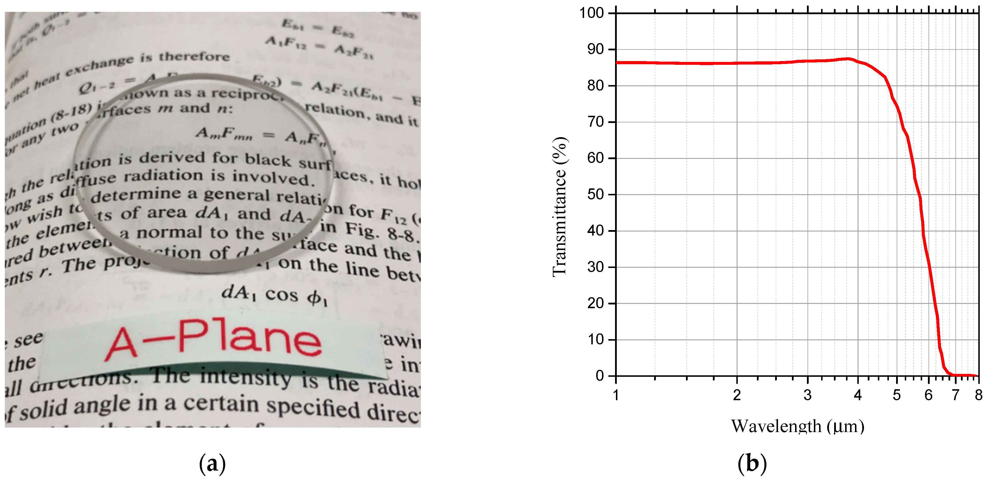
3.2. Specimen for Measurement

This study aims to develop a technology to measure the thermophysical properties of transparent anisotropic materials. To verify this measurement method, an appropriate specimen needs to be selected. In this study, an emphasis was placed on selecting a material, which has literature values and is used in various fields, as the object of the verification. Therefore, 3 mm-thick A-plane sapphire glass was selected as the specimen (Figure 7a). Sapphire glass has excellent mechanical and heat transfer properties as well as high light transmittance over a broad range of wavelengths, as shown in Figure 7b. Therefore, it has been widely used in various industries, including transparent displays [43]. Also, for such reasons, it was easy to obtain the specimen in appropriate size and form to the research.

As shown in Figure 8, sapphire glass is classified as C-plane, A-plane, or R-plane depending on the crystal orientation [43], and the anisotropic properties vary depending on this orientation. In this study, A-plane sapphire glass was used.

Table 5. Literature values of thermal conductivity for sapphire glass.

$\mathbf{Thermal}\mathbf{Conductivity}(\mathit{W}/(\mathit{m}\mathit{K}))$		Measurement Temperature $(\mathit{K})$	Literature Author	Average Value $(\mathit{W}/(\mathit{m}\mathit{K}))$
x-dir ($k_{1,11}$) and z-dir ($k_{1,33}$)	32.5	298	Dobrovinskaya et al [43]	36.4 ($\pm$ 8.5)
	25.2	300	Ho et al [44]
	47	298	Kinoshita et al [45]
	42.3	303	Knapp [46]
	35	300	Darwish et al [47]
y-dir ($k_{1,22})$	30.3	298	Dobrovinskaya et al [43]	27.1 (± 4.1)
	23.1	300	Ho et al [44]
	31	298	Kinoshita et al [45]
	24	300	Schmid et al [48]

summarizes ${\mathrm{k}}_{11}$, ${\mathrm{k}}_{22}$, and ${\mathrm{k}}_{33}$ of A-plane sapphire glasses presented in various literature [43,44,45,46,47,48]. In the numerical analysis, ${\mathrm{k}}_{11}$, ${\mathrm{k}}_{22}$, and ${\mathrm{k}}_{33}$ were selected as 32.5, 23.1, and 32.5 $\mathrm{W}/\left(\mathrm{mk}\right)$ from various literature.

Table 6. Properties of A-Plane Sapphire.

$\mathbf{Density}(\rho ,kg/m^3)$		3980
Specific heat capacity$(c_P,J/(kg\cdot K))$		761
Thermal conductivity $(k,W/(mK))$	x-dir ($k_{1,11}$)	32.5
	y-dir ($k_{1,22})$	23.1
	z-dir ($k_{1,33}$)	32.5
Absorption coefficient $(\lambda ,m^{-1})$		653.05
Thermo-optical coefficient $(dn/dT,k^{-1})$		1.30 × 10−5

shows the thermal and optical properties of the sapphire glass used in this numerical analysis [43,49].

3.3. Parameter for Experiment

Through the experiment, the thermal conductivities of A-plane sapphire glass in the principal axis directions ($k_{11}$, $k_{22}$) were measured, and the results were compared with the values in the existing literature to verify the transparent anisotropic collinear method. To this end, the modulation frequency of the pump beam, the radius of the pump beam, the radius of the probe beam, the relative position, and the travel distance between the measurement points were summarized as shown in

Table 7. Experimental setup value.

Frequency (Hz)	20
Radius (mm)	82.5
Relative position (Numerical) (mm)	0.15~0.5 (interval: 0.02)
Relative position (Experimental) (mm)	0.15~0.5 (interval: 0.02)

. When the relative position between the probe beam and the pump beam was very small (0–0.15 mm), it was excluded because it could cause errors in the phase delay measurement. 2400 phase delay values were obtained for 120 s to determine the phase delay value at one relative position. The arithmetic mean of these data in the 95% confidence interval was used as the representative value.

4. Results and Discussion

Figure 9 shows the phase delay in each measurement direction ($\theta$: $0°$, $30°$, $45°$, $60°$, and $90°$) according to the relative position. The black lines represent the values derived through theoretical analysis (temperature field derivation through numerical analysis and phase delay calculation using Equations (12) and (13)) using the properties in Table 6, and the square points represent the values derived through the experiment. The experimental results are shown along with error bars. An error bar represents the standard deviation of the 95% interval data among the obtained 2400 phase delay values at one relative position.

It was found that the experimental and numerical analysis results had similar tendencies and were in good agreement. The experimental results showed that the error was relatively higher due to the influence of the pump beam in the area where the distance between the pump beam and the probe beam was small (near 0.15 mm), as explained above. On the other hand, in the area where the distance between the pump beam and the probe beam was large (near 0.50 mm), the error was relatively higher because the accuracy of the phase difference acquisition was reduced due to the low temperature gradient in the material.

Using the experimental results, it is possible to determine the thermal conductivity through the phase curve method algorithm explained above through Figure 5. From the theoretical phase delay results derived while the thermal conductivity ($k_{rand}$) was varied and the phase delay results derived from the experiment, the RMSE was derived using Equation (14). Figure 10 shows the RMSE according to the thermal conductivity substituted into theoretical analysis for various measurement directions ($\theta$: $0°$, $30°$, $45°$, $60°$, and $90°$).

$$RMSE=\sqrt{\frac{{\displaystyle \sum _{i=1}^N{({\chi }_{cal}-{\chi }_{\exp })}^2}}{N}}(N=\mathrm{Relative}\mathrm{positions})$$

(14)

Based on these results, Figure 11 shows the thermal conductivity according to the measurement direction derived using the transparent anisotropic collinear method, the average of literature values in the principal axis directions ($k_{11}$, $k_{22}$), and the calculated values that can be derived through the vector operation of Equation (10).

It was found that the measurement values were accurate because absolute errors from the thermal conductivity of A-plane sapphire glass in the principal axis direction from various literature were less than about 4 $\mathrm{W}/\left(\mathrm{m}\mathrm{K}\right)$. It was also found that the thermal conductivity according to the measurement direction was accurate because errors from the values calculated based on the average of literature values were less than 4 $\mathrm{W}/\left(\mathrm{m}\mathrm{K}\right)$.

Table 8. Measurement results of A-plane sapphire using collinear deflection method.

Measurement angle(deg)	0	30	45	60	90
Literature value$(W/mK)$	36.40 ($\pm$8.5)	34.10 (± 7.4)	31.75 (± 6.3)	29.43 (± 5.2)	27.10 (± 4.1)
Measurement value$(W/mK)$	32.23	29.97	28.17	25.58	23.54
Root mean square error(deg)	3.3	5.52	3.18	4.47	2.97
Absolute error$(W/mK)$	4.17	4.13	3.58	3.85	3.56

summarizes the measured values and errors.

5. Conclusions

In this study, a transparent anisotropic collinear deflection method was proposed to measure the thermal properties of transparent anisotropic materials, which could not be measured using the existing photothermal deflection methods. To this end, numerical analysis and experimental study were conducted for a single layer anisotropic material, and the following conclusions could be drawn.

• Based on the 3D heat conduction equation to which the anisotropic thermal conductivity with the orthorhombic structure was applied, the temperature distribution of the anisotropic material was derived using a complex transformation method and numerical analysis, and it was verified through a comparison with the analytical solution of the well-known mirage deflection method. Deflection analysis was conducted to measure the thermal conductivity of the transparent anisotropic material by applying the derived temperature distribution.
• The measurement method proposed in this study was verified by measuring the effective thermal conductivity according to the principal thermal conductivity directions ($k_{11}$, $k_{22}$) and measurement directions using A-plane sapphire glass whose $k_{11}$, $k_{22}$, and $k_{33}$ were known to be 36.4, 27.1, and 36.4 W/(mk) from the various literatures.
• The phase curve method algorithm was applied to derive the thermal conductivity of the measurement specimen using the phase curve results according to the relative position (distance between the pump beam and the probe beam) derived from the experiment. The RMSE ranged from 2.97 to 5.25° depending on the measurement direction.
• It was confirmed that the measured thermal conductivity according to the finally derived direction ($\theta$) had absolute errors less than about 4 W/(mk) when compared with the average of literature values.

In this study, a method for measuring the thermal conductivity of a material with transparent anisotropic properties was proposed. However, it was found that the RMSE derived by applying the phase curve method was relatively high. This appears to be because sufficient heat could not be supplied due to the specificity of the material (high transparency), and thus a low temperature field ($dT$= 2–3 °C) was generated. It is thought that this problem can be solved by applying materials with high light absorption to the surface. In future research, a measurement method capable of overcoming this drawback will be proposed.

References

1. Oktay, S.; Hannemann, R.; Bar-Cohen, A. High heat from a small package. Mech. Eng. (USA) 1986, 108, 36–42. [Google Scholar]
2. Nakayama, W. Thermal management of electronic equipment: A review of technology and research topics. Appl. Mech. Rev. 1986, 39, 1847–1868. [Google Scholar] [CrossRef]
3. Incropera, F. Convection heat transfer in electronic equipment cooling. J. Heat Transf. 1988, 110, 1097–1111. [Google Scholar] [CrossRef]
4. Bar-Cohen, A. Thermal management of electronic components with dielectric liquids. JSME Int. J. Ser. B Fluids Therm. Eng. 1993, 36, 1–25. [Google Scholar] [CrossRef]
5. Kubo, W.; Fujikawa, S. Embedding of a gold nanofin array in a polymer film to create transparent, flexible and anisotropic electrodes. J. Mater. Chem. 2009, 19, 2154–2158. [Google Scholar] [CrossRef]
6. Bae, S.; Kim, H.; Lee, Y.; Xu, X.; Park, J.-S.; Zheng, Y.; Balakrishnan, J.; Lei, T.; Kim, H.R.; Song, Y.I. Roll-to-roll production of 30-inch graphene films for transparent electrodes. Nat. Nanotechnol. 2010, 5, 574–578. [Google Scholar] [CrossRef] [Green Version]
7. Mietta, J.L.; Ruiz, M.M.; Antonel, P.S.; Perez, O.E.; Butera, A.; Jorge, G.; Negri, R.M. Anisotropic magnetoresistance and piezoresistivity in structured Fe3O4-silver particles in PDMS elastomers at room temperature. Langmuir 2012, 28, 6985–6996. [Google Scholar] [CrossRef]
8. Uetani, K.; Okada, T.; Oyama, H.T. Thermally conductive and optically transparent flexible films with surface-exposed nanocellulose skeletons. J. Mater. Chem. C 2016, 4, 9697–9703. [Google Scholar] [CrossRef]
9. Powell, R.; Taylor, R. Multi-Property Apparatus and Procedure for High Temperature Determinations; Purdue Univ., Lafayette, Ind.: West Lafayette, IN, USA, 1970. [Google Scholar]
10. Taylor, R.; Kimbrough, W.; Powell, R. Thermophysical properties of tantalum, tungsten, and tantalum-10 wt. per cent tungsten at high temperatures. J. Less Common Met. 1971, 24, 369–382. [Google Scholar] [CrossRef]
11. Taylor, R. Determination of thermophysical properties by direct electric heating. High Temp. High Press. 1981, 13, 9–22. [Google Scholar]
12. Cezairliyan, A.; Morse, M.; Beckett, C. Measurement of melting point and electrical resistivity (above 2840 deg K) of molybdenum by a pulse heating method. Rev. Int. Des Ht. Temp. Et Des Refract. 1970, 7, 382–388. [Google Scholar]
13. Cezairliyan, A. Design and operational characteristics of a high-speed (millisecond) system for the measurement of thermophysical properties at high temperatures. J. Res. Nat. Bur. Stand.(US) C 1971, 75, 7–18. [Google Scholar] [CrossRef]
14. Cezairliyan, A.; Miiller, A. Specific heat capacity and electrical resistivity of a carbon-carbon composite in the range 1500–3000 k by a pulse heating method. Int. J. Thermophys. 1980, 1, 317–326. [Google Scholar] [CrossRef]
15. Sell, J. Photothermal Investigations of Solids and Fluids; Academic Press INC.: Boston, MA, USA, 1989. [Google Scholar]
16. Cahill, D.G.; Katiyar, M.; Abelson, J. Thermal conductivity of a-Si: H thin films. Phys. Rev. B 1994, 50, 6077. [Google Scholar] [CrossRef]
17. Vozár, L.; Hohenauer, W. Flash method of measuring the thermal diffusivity. A review. High Temp.-High Press. 2004, 36, 253–264. [Google Scholar] [CrossRef]
18. Jackson, W.B.; Amer, N.M.; Boccara, A.; Fournier, D. Photothermal deflection spectroscopy and detection. Appl. Opt. 1981, 20, 1333–1344. [Google Scholar] [CrossRef] [PubMed]
19. Fournier, D.; Boccara, C.; Skumanich, A.; Amer, N.M. Photothermal investigation of transport in semiconductors: Theory and experiment. J. Appl. Phys. 1986, 59, 787–795. [Google Scholar] [CrossRef]
20. Spear, J.D.; Russo, R.E.; Silva, R.J. Collinear photothermal deflection spectroscopy with light-scattering samples. Appl. Opt. 1990, 29, 4225–4234. [Google Scholar] [CrossRef] [PubMed]
21. Salazar, A.; Sánchez-Lavega, A.; Fernandez, J. Thermal diffusivity measurements in solids by the ‘‘mirage’’technique: Experimental results. J. Appl. Phys. 1991, 69, 1216–1223. [Google Scholar] [CrossRef]
22. Bertolotti, M.; Liakhou, G.; Li Voti, R.; Peng Wang, R.; Sibilia, C.; Yakovlev, V. Mirror temperature of a semiconductor diode laser studied with a photothermal deflection method. J. Appl. Phys. 1993, 74, 7054–7060. [Google Scholar] [CrossRef]
23. Rantala, J.; Wei, L.; Kuo, P.; Jaarinen, J.; Luukkala, M.; Thomas, R. Determination of thermal diffusivity of low-diffusivity materials using the mirage method with multiparameter fitting. J. Appl. Phys. 1993, 73, 2714–2723. [Google Scholar] [CrossRef]
24. Spear, J.D.; Silva, R.J.; Klunder, G.L.; Russo, R.E. Collinear photothermal deflection spectroscopy of liquid samples at varying temperature. Appl. Spectrosc. 1993, 47, 1580–1584. [Google Scholar] [CrossRef]
25. Salazar, A.; Sánchez-Lavega, A.; Fernández, J. Thermal diffusivity measurements on solids using collinear mirage detection. J. Appl. Phys. 1993, 74, 1539–1547. [Google Scholar] [CrossRef]
26. Bertolotti, M.; Liakhou, G.; Ferrari, A.; Ralchenko, V.; Smolin, A.; Obraztsova, E.; Korotoushenko, K.; Pimenov, S.; Konov, V. Measurements of thermal conductivity of diamond films by photothermal deflection technique. J. Appl. Phys. 1994, 75, 7795–7798. [Google Scholar] [CrossRef]
27. Salazar, A.; Sánchez-Lavega, A. Low temperature thermal diffusivity measurements of gases by the mirage technique. Rev. Sci. Instrum. 1999, 70, 98–103. [Google Scholar] [CrossRef]
28. Li, B.; Gupta, R. Simultaneous measurement of absorption coefficient, thermal diffusivity, and flow velocity in a gas jet with pulsed photothermal deflection spectroscopy. J. Appl. Phys. 2001, 89, 859–868. [Google Scholar] [CrossRef]
29. Jeon, P.; Lee, E.; Lee, K.; Yoo, J. A theoretical study for the thermal diffusivity measurement using photothermal deflection scheme. Energy Eng. J. 2001, 10, 63–70. [Google Scholar]
30. Salazar, A.; Gateshki, M.; Gutiérez-Juárez, G.; Sánchez-Lavega, A.; Ang, W.T. Novel results on collinear mirage deflection. Anal. Sci. 2001, 17, 95–98. [Google Scholar]
31. Iravani, M.V.; Nikoonahad, M. Photothermal waves in anisotropic media. J. Appl. Phys. 1987, 62, 4065–4071. [Google Scholar] [CrossRef]
32. Quelin, X.; Perrin, B.; Louis, G.; Peretti, P. Three-dimensional thermal-conductivity-tensor measurement of a polymer crystal by photothermal probe-beam deflection. Phys. Rev. B 1993, 48, 3677. [Google Scholar] [CrossRef]
33. Salazar, A.; Sánchez-Lavega, A.; Ocáriz, A.; Guitonny, J.; Pandey, J.; Fournier, D.; Boccara, A. Novel results on thermal diffusivity measurements on anisotropic materials using photothermal methods. Appl. Phys. Lett. 1995, 67, 626–628. [Google Scholar] [CrossRef]
34. Salazar, A.; Sánchez-Lavega, A.; Ocariz, A.; Guitonny, J.; Pandey, G.; Fournier, D.; Boccara, A. Thermal diffusivity of anisotropic materials by photothermal methods. J. Appl. Phys. 1996, 79, 3984–3993. [Google Scholar] [CrossRef]
35. Murphy, J.C.; Spicer, J.M.; Aamodt, L.C.; Royce, B.S. Photoacoustic and photothermal phenomena II. Baltimore, Maryland, July 31–August 3, 1989. Available online: https://link.springer.com/book/10.1007/978-3-540-46972-8 (accessed on 10 April 2019).
36. Lee, K.; Kang, J.; Jeon, P.; Jo, B.; Yoo, J.; Kim, H. Measurement of thermal conductivity for single-and bilayer materials by using the photothermal deflection method. J. Korean Phys. Soc. 2007, 51, 36. [Google Scholar] [CrossRef]
37. Jeon, P.; Kim, J.; Kim, H.; Yoo, J. Thermal conductivity measurement of anisotropic material using photothermal deflection method. Thermochim. Acta 2008, 477, 32–37. [Google Scholar] [CrossRef]
38. Ross, R.B. Metallic Materials Specification Handbook; Springer Science & Business Media: Berlin, Germany, 2013. [Google Scholar]
39. Carslaw, H.S.; Jaeger, J.C. Conduction of Heat in Solids; Clarendon Press: Oxford, UK, 1960. [Google Scholar]
40. McKie, C.; McKie, D. Newnham. Structure-Property Relations (Crystal Chemistry of Non-Metallic Materials, Vol. 2). Mineral. Mag. 1977, 41, 143–144. [Google Scholar] [CrossRef]
41. Putnis, A. An Introduction to Mineral Sciences; Cambridge University Press: Cambridge, UK, 1992. [Google Scholar]
42. Lovett, D. Tensor Properties of Crystals; CRC Press: Boca Raton, FL, USA, 2018. [Google Scholar]
43. Dobrovinskaya, E.R.; Lytvynov, L.A.; Pishchik, V. Sapphire: Material, Manufacturing, Applications; Springer Science & Business Media: Berlin, Germany, 2009. [Google Scholar]
44. Ho, C.Y.; Powell, R.W.; Liley, P.E. Thermal Conductivity of the Elements: A Comprehensive Review. J. Phys. Chem. Ref. Data 1974, 3, 1–30. [Google Scholar]
45. Kinoshita, H.; Otani, S.; Kamiyama, S.; Amano, H.; Akasaki, I.; Suda, J.; Matsunami, H. Zirconium diboride (0001) as an electrically conductive lattice-matched substrate for gallium nitride. Jpn. J. Appl. Phys. 2001, 40, L1280. [Google Scholar] [CrossRef]
46. Knapp, W. Thermal conductivity of nonmetallic single crystals. J. Am. Ceram. Soc. 1943, 26, 48–55. [Google Scholar] [CrossRef]
47. Darwish, A.M.; Bayba, A.J.; Hung, H.A. Thermal resistance calculation of AlGaN-GaN devices. IEEE Trans. Microw. Theory Tech. 2004, 52, 2611–2620. [Google Scholar] [CrossRef]
48. Schmid, F.; Rogers, H.H.; Khattak, C.P.; Felt, D.M. Growth of very large sapphire crystals for optical applications. Inorg. Opt. Mater. 1998, 3424, 3–47. [Google Scholar]
49. Hagemann, H.-J.; Gudat, W.; Kunz, C. Optical constants from the far infrared to the x-ray region: Mg, Al, Cu, Ag, Au, Bi, C, and Al2O3. JOSA 1975, 65, 742–744. [Google Scholar] [CrossRef]
Figure 1. Photothermal deflection method types. (a) Mirage deflection method. (b) Collinear deflection method.
Applsci 09 01522 g001
Figure 2. Schematic of phase delay.
Applsci 09 01522 g002
Figure 3. Schematic diagram of collinear deflection analysis.
Applsci 09 01522 g003
Figure 4. Comparison of analytical and numerical solutions. (a) Temperature change in x-direction ( y = 0 ,   z = 0 ). (b) Temperature change in z-direction ( x = 0 ,   y = 0 ).
Applsci 09 01522 g004
Figure 5. Algorithm for determination of thermal conductivity.
Applsci 09 01522 g005
Figure 6. Schematic of experimental setup.
Applsci 09 01522 g006
Figure 7. Characteristic of specimen for measurement. (a) A-plane sapphire (3 mm thick). (b) Transmittance curve of A-plane sapphire.
Applsci 09 01522 g007
Figure 8. Crystal orientation of sapphire glass.
Applsci 09 01522 g008
Figure 9. Comparison of experimental and theoretical results for various measurement directions. (a) θ = 0 ° . (b) θ = 30 ° . (c) θ = 45 ° . (d) θ = 60 ° . (e) θ = 90 ° .
Applsci 09 01522 g009
Figure 10. RMSE of thermal conductivity determination algorithm. (a) θ = 0 ° . (b) θ = 30 ° . (c) θ = 45 ° . (d) θ = 60 ° . (e) θ = 90 ° .
Applsci 09 01522 g010aApplsci 09 01522 g010b
Figure 11. Experimental results for various measurement directions.
Applsci 09 01522 g011