Abstract
Improvements in sustainability at the farm level are the basic driver of agricultural sustainability at the macro level. This is a challenge that can only be met by farms which efficiently process inputs into products. The increase in the efficiency of European farms is largely conditioned by measures taken under the Common Agricultural Policy (CAP), especially its second pillar. The purpose of this study was to determine the net effect of pro-investment instruments available under the second pillar of the CAP in selected Central and Eastern European countries. Unpublished Farm Accountancy Data Network (FADN) microdata provided by the European Commission’s Directorate-General for Agriculture and Rural Development (DG AGRI) were used as the source material. The study presented in this paper is unique in that the research tasks are based on unpublished microdata of selected Central and Eastern European farms. The study relied on the Propensity Score Matching approach; the net effect of pro-investment mechanisms was analyzed using productivity and profitability indicators calculated for farms which have been keeping FADN records for a continuous period of no less than 6 years. As shown by the study, structural funds available under the CAP clearly provided an investment incentive for farms. The conclusion from the assessment of changes in the availability of productive inputs is that the beneficiaries reported a greater increase in fixed asset value and in farm area in all countries except for the Czech Republic and Slovakia. The comparative analysis of countries covered by this study failed to clearly confirm that labor is substituted with capital to a significant extent. Every country covered by this study experienced a noticeable negative net effect on both the productivity and profitability of capital. When considering all the countries, the beneficiary group has no clear advantage over the control group in terms of changes in land and labor productivity and profitability (a statistically significant positive effect was recorded for land productivity and profitability in Slovenia). As regards labor, a statistically significant positive net effect (a difference in growth rate between the beneficiary group and the control group) was recorded in Slovenia, but also in Poland, where beneficiary farms reported a greater increment in labor profitability and reduced the negative difference in labor productivity.
1. Introduction
The main challenge faced by agriculture is to provide the population with the food and other bio-products necessary for their development while protecting natural capital, which means using it in a sustainable way [1]. Improvements in sustainability at the farm level are the basic driver of agricultural sustainability at the macro level [2], which means performing stable, economically viable, socially accepted and environmentally sound production activity. Hence, sustainable farm development depends on three main factors: economic, environmental and social factors. The attainment of sustainability at the farm level is largely based on economic sustainability, which is expressed by actions such as investing and reaping the related economic outcomes (which drive improvements in sustainability). However, as Savickienė and Miceikienė [3] emphasize, when dealing with farm sustainability, researchers mostly focus on the environmental and social aspects while neglecting the impact of the economic factor. Nevertheless, as shown by the literature review [4,5], the economic factor is of key importance to sustainable farm development because the other two factors depend on it. Ensuring an adequate level of production profitability is the only way to encourage farmers to take better care of the environment which, in turn, can translate into improvements in the population’s standards of living, as emphasized by Savickienė and Miceikienė [3]. This is a challenge that can only be met by farms which efficiently process inputs into products [6]. Improvements in productivity—i.e., greater output per unit of input—result in reducing harmful pressures on the environment and improving profitability either by enhancing productivity or by reducing costs [7]. Many countries rely on a broad spectrum of intervention instruments to support the sustainable development of the agricultural sector because of its particularities.
In European Union countries, government intervention in agriculture is underpinned by the Common Agricultural Policy, which was designed primarily to ensure sustainable agricultural development by pursuing social, economic and environmental goals [6], and the farms are covered by a series of its intervention mechanisms. Since 2000, the Common Agricultural Policy has been composed of two pillars. The objectives of the first one include supporting farm incomes and promoting environmental sustainability and animal welfare. The second pillar involves structural measures (mostly including investment support) which take into account the particularities and rural development requirements of each EU member country [8]. In that context, a highly important outcome of investment measures taken under the CAP is the implementation of state-of-the-art technologies which contribute to environmental protection and counteract adverse climate change; this is how they meet the priority goals sought by the Community, which intends to stop adverse climatic changes. The European Union encourages farmers to employ environmentally friendly solutions [9], rewarding environmental enhancements with investment subsidies.
European Union countries differ from each other in the size and structure of their agricultural output, including crop yields, unit livestock productivity ratios and the size and structure of inputs. As a consequence, they also differ in economic performance [10]. There are many reasons behind the differences in the resource, production and economic situations of farms [11,12]. According to many authors [13,14,15,16], Common Agricultural Policy instruments are increasingly often the cause of these gaps between countries. In this context, it is worthy of note that member countries differ in how long they have been covered by CAP instruments (depending on when they joined the EU). The newest members (who joined the Community after 2000) mainly include Central and Eastern European countries, who differ from the “old” Union in terms of their agricultural policies and the economic developments experienced in recent years [17]. They have now been covered by the implementation of CAP measures for more than ten years. The above situation makes it even more imperative to assess the effectiveness of these mechanisms on the changes in the economic situation of farms in these countries.
Structural measures which promote farm modernization and restructuring play an important role in member countries who joined the EU in 2004. This is because, as regards the techniques and technologies employed and the advancement of structural transformation processes [18,19,20], they lag considerably behind countries who underwent the necessary changes in the post-war period [21,22,23]. The objective of investment support under the CAP is to overcome the many factors that restrict the farms’ capacity to incur significant investment expenditure. Therefore, since the implementation of pre-accession mechanisms to this day, support for farm development investments has been among the key instruments of the agricultural transformation process [24]. This enables a faster implementation of technical, biological and organizational advancements which, in turn, contribute to increasing the agricultural production potential and driving improvements in the farms’ economic performance [25,26,27]. The expected outcome of investment mechanisms available under the second pillar of the CAP is an improvement in productivity and economic performance at farm level [28]. This is because modern agriculture requires capital [29]. Investment decisions affect both current and future production [30]. Taking into consideration the limited access to capital due to the unique characteristics of agricultural sectors throughout the world [31,32,33], many governments see it as their responsibility to assist farmers in obtaining capital. Agricultural programs in developed market economies, such as Western Europe, have evolved over the years and have been rationalized as interventions to correct market failures [29]. Similarly, Barry and Robinson [32] assume that the policy element of agricultural finance considers the role of governments in filling the gaps and resolving imperfections in the agricultural finance markets and in providing targeted assistance to designated recipients. The importance of CAP investment mechanisms to the development of farms was also emphasized by Guastella et al. [34] and Czubak and Sadowski [35]. For instance, in Poland, agricultural investments doubled after the accession to the EU. This contributed to improving the availability of fixed assets in farms [36]. However, the countries differ considerably in how they implement CAP investment measures [37] which, in turn, can affect the possible impacts of interventions on the renewal and development of the farms’ technical assets.
A situation in which the farms become highly dependent upon subsidies could undermine the improvements in productivity and efficiency; that fact also makes it reasonable to address the impacts of intervention mechanisms designed to promote investments [38]. The metrics of efficiency include technical efficiency—a concept which means that an enterprise should seek to maximize output under the assumption that a defined level of input is available [39]. As shown by a literature review, that aspect was addressed by several researchers who endeavored to determine the relationship between agricultural subsidies and technical efficiency; however, they ended up with contrasting findings [40]. For instance, in their meta-analysis comprising 70 different studies spanning over a period of circa 30 years, Minviel and Latruffe [41] demonstrated that agricultural subsidies had a significant negative impact on the farms’ technical efficiency. However, on the other hand, a number of papers exist that confirm the positive effect of subsidies on farm efficiency [42,43,44]. These contradictions could result from differences in agricultural characteristics between the countries, and from structural differences between intervention mechanisms [45]. The dual impact of subsidies on changes in efficiency is particularly noticeable in the case of payments decoupled from production volumes [46]. Various types of subsidies can result in different impacts on farms, and hence can have different effects on their efficiency and profitability [47].
The diverse impacts are also confirmed in studies by Bonfiglio [40], who found that the effect of subsidies on the farms’ technical efficiency can differ in terms of the function of factors, including their type of farming. Despite these highly interesting findings, the authors point to certain imperfections in their studies. First of all, there are some reservations as to the analysis period, which was only one year. The authors believe that a longer time perspective could yield more reliable findings [40]. Therefore, unlike their research project, the analysis presented in this paper covers a broader time frame (12 years) and a larger territory (eight countries). According to some studies, while subsidies can drive an increase in input productivity, this mainly depends on their nature [45]. Therefore, this paper focuses on investment mechanisms which can enhance productivity and reduce costs (and, as a consequence, improve profitability), as confirmed by numerous studies, including those by Boulanger and Philippidis [47] and Dudu and Kristkova [48].
This paper relied on micro-data from the Farm Accountancy Data Network (FADN) operated by DG-AGRI. According to Michalek [49], FADN is the only data source suitable for research based on the counterfactual approach, including the Propensity Score Matching used in this study. The European FADN was established in European Economic Community countries upon the implementation of Common Agricultural Policy mechanisms. Note that only commercial farms are monitored by the system. While findings from research based on FADN micro-data (such as this paper) are available, they relate solely to single regions or countries [49,50]. Importantly, the authors cited above consider the counterfactual method used in this paper to be suitable for assessing the Rural Development Programs implemented by the EU, including the intervention measures taken to promote investments. In practice, the following four alternative methods, referred to as naïve methods, are generally used in evaluating the EU programs [49]: (1) observing only the beneficiaries of aid prior to, and following the receipt of, subsidies (this approach fails to take account of other impacts on the change in the situation); (2) comparing the group of beneficiaries with all other operators; or (3) comparing the group of beneficiaries with an averaged group composed of beneficiaries and non-beneficiaries (these approaches fail to take account of comparability between groups which may be composed of operators with different characteristics); and (4) a method which consists of comparing the beneficiary group with a random control group (without matching, which also makes the groups non-comparable). Unlike the above methods, PSM enables the examination of the net effect of interventions by comparing two groups (the beneficiaries and the control group) which share similar characteristics based on the selected variables.
This paper contributes to the literature by determining the changes in the production and income efficiency of farms resulting from the implementation of investment mechanisms under the CAP. Despite many attempts and a number of dedicated studies, scientific discussion is still ongoing because no clear answer has yet been provided to the question of the impacts of intervention mechanisms (including investment measures) on the broadly defined economic condition of farms. This study was designed to answer the following research questions: what is the impact of investment intervention mechanisms on the situation of farms as regards changes in productive inputs (labor, land and capital), the relationships between them and the production and income performance? Are there any significant differences between the beneficiaries of investment support programs and farms which do not access these programs? Are there any significant differences between the countries in terms of the production and income-related effects of the implementation of investment mechanisms under the second pillar of the CAP? Answers to these questions are sought through an analysis of productivity and profitability indicators of labor, land and capital.
2. Materials and Methods
Unpublished FADN microdata provided by the European Commission’s DG AGRI were used as the source material. The study presented in this paper is unique in that the research tasks are based on unpublished microdata of selected Central and Eastern European farms. The microeconomic nature of this data also makes it possible to carry out dynamic analyses [51]. Formal guidelines for working with extremely sensitive data are highly restrictive, and therefore this paper only presents aggregated results for 15 farms. The research covered selected Central and Eastern European countries: Czech Republic, Estonia, Lithuania, Latvia, Poland, Slovakia, Slovenia and Hungary. For the purposes of this research, the countries were selected because of their geographic location and (mostly) because they joined the EU in the same year. Of the countries who joined the EU in 2004, Cyprus and Malta were excluded because (as shown by previous own research and a study of the relevant literature) their agriculture is substantially different and unique. The study period was 2004–2015. The initial year marks the first enlargement of the EU with CEE countries, while the last year corresponds to the most recent data from FADN resources. Agricultural accounting data are subject to a multi-stage verification process at farm, national and European Commission levels and are therefore made available only after a delay. Hence, 2015 was the last period surveyed.
The implementation of agricultural policies entails heavy expenditure, and public funds must therefore be disbursed to provide investment support. The implementation of relevant measures needs to be evaluated to determine the actual benefits brought by specific instruments. The main purpose of the evaluation is to improve the effectiveness, quality and coherence of the implemented programs [52]. Support to the investment and modernization of agricultural holdings is a capital subsidy that aims to encourage agricultural firms to undertake more gross investment in plants, machinery, and new production equipment on the assumption that this results in increased productivity and output [25]. Hence, it is important to determine the outcomes brought by the implementation of these instruments, which is the main research goal of this paper.
In practice, the evaluation of political interventions proves to be a difficult task [53]. The analytical difficulty is the assessment of the causative link, i.e. the attribution of changes to the implemented policy. The problem of causality was addressed by a number of researchers, including Fisher, Neyman, Cochran, Cox, Heckman, Roy, Quandt and Rubin [54]. The randomized controlled experiment is a recognized method for the assessment of causative links [55]. However, in economic analyses, experiments seem to be extremely difficult, if not impossible, because of numerous technical, social or ethical restrictions. In such cases, efforts should be made to assign the characteristics of an experimental set to the available dataset. This can be done by combining data, in particular by using the Propensity Score Matching method [56,57].
When interpreting the results of economic analyses, it is very helpful to compare the figures with reference entities or to make a time comparison (from 2004 onwards) or a regional comparison (within eight CEE countries). In this research, the above is of key importance in order to answer the question of how the selected agricultural interventionism mechanisms affect the microeconomic situation of farms in different countries. In other words, the purpose of the analysis was to determine the net effect of selected measures in particular countries (Figure 1).
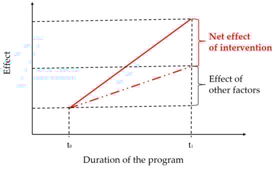
Figure 1.
Determining the net effect of Common Agricultural Policy (CAP) pro-investment measures. Source: own study.
This effect may be estimated by comparing the average economic performance of farms covered by structural support with that recorded in the control group. The reference group included similar operators selected based on their resources of productive inputs: labor, land and capital. The analysis was based on Propensity Score Matching (PSM). As a consequence, it was possible to compare microeconomic data between beneficiaries of structural funds and their counterparts from the control pool.
All farms covered were divided into the beneficiaries’ pool and the control pool as per the formula below
where
- PIM: pro-investment measures;
- SIV: investment subsidies (SE406 in the FADN).
Accordingly, the control pool was composed of farms which did not access any investment support under the second pillar of the CAP in the entire study period (2004–2015) but, at the same time, they met the minimum requirements for investment support measures (including the minimum economic size or maximum acreage). This is how the second methodological assumption was met, which requires that each farm have equal opportunities in applying for investment subsidies. In turn, experimental farms were those which accessed support for the first time in year t1, with the total amount of support in the following 5 years being no less than EUR 5,000. A large proportion of farms was eliminated because of the unavailability of continuous records in the FADN database within a period of no less than 6 years. This study used a 6-year analysis period, which is consistent with program requirements for the minimum sustainability of investment, plus one year preceding the investment. The population of the experimental and control pools was as follows (Table 1).

Table 1.
Number of farms in the experimental and control pools.
The initial situation of, and the differences between, the two groups of farms (the beneficiaries and the control group) were determined for the year before the use of pro-investment funds (t0). This allowed us to avoid the distorting impact of the pro-investment subsidies received on the farms’ economic standing (which is an essential part of this research). The input variables of the PSM vector were set as utilized agricultural area in hectares (SE025), labor input in AWU (Annual Work Unit, SE010) and gross fixed assets other than land (SE441–SE446). As a consequence, the paired farms had a similar production potential (a similar value of productive inputs) in year t0. In year t1, one of them started to access pro-investment funds (the experimental group) while the other one (the control group) did not. This resulted in the creation of two equally sized groups for each country. The difference in the size of the groups between the countries is mostly due to the difference in the continuous presence of respective farms in the FADN database. For instance, the Polish FADN includes 3964 farms with continuous entries from 2004 to 2015, whereas in Lithuania, continuous data were available only for 23 farms. The number of farms which have been keeping records in the FADN database for a 6-year period reached the required minimum (15) in all countries. Hence, it is possible to present the results for all of them.
The matching-based estimation consists of analyzing the counterfactual conditions, i.e., the hypothetical values of the outcome variable. When considering the impact of a treatment on the outcome variable, calculating the magnitude of that impact means determining the effect one treatment would have had on a unit which, in fact, received some other treatment [58]. Therefore, in the counterfactual approach, the outcome variable may be defined as [59,60]
where
- Yi: the value of the outcome variable for unit i;
- Yi1, Yi0: the values of the outcome variable in the case where unit i either received a treatment or did not receive it (respectively);
- Di: a Boolean variable, which is 0 if unit i did not receive the treatment, or 1 otherwise.
The effect of the treatment on the outcome variable considered may be determined at the level of a single observation as per the following formula
In fact, variable D may only have one of two possible values, and therefore only one of the outcomes may be observed (Yi1 or Yi0). Under the assumption that Yi1 is known, no information is available on Yi0. This situation is referred to by Rubin et al. [61] and Heckman et al. [62] as the missing data problem. One way to solve this is to consider the counterfactual conditions, i.e., the estimations which approximate the non-observable values of the variables
where and are the estimated potential values of the outcome variable in the case where unit i either did not receive a treatment or did receive it (respectively).
Many authors, including Holland [63], refer to the static solution, which consists of shifting from the unit level to the level of the population to which that unit belongs. Let WATE be the average treatment effect (ATE) for population I. In accordance with earlier assumptions for the unit causal effect, the following is true
Or
where E(Y1) is the average effect in a situation where all units across the population received the treatment, and E(Y0) is the average effect in a situation where all units are included in the control group. In order to assess specific actions, a researcher must focus only on the effect experienced by units subject to intervention. In this situation, the treatment on treated effect (Average Treatment of Treated) is sought, and may be expressed as follows [60]
where
- E(Y1 | D = 1): the average outcome of the intervention in the group of units which received the treatment.
- E(Y0| D = 1): the average outcome of the absence of intervention in the group which received the treatment.
E(Y0| D = 1) is the non-observable (counterfactual) effect, which, however, may be estimated. In fact, (Y0| D = 0) is known. This is the average effect experienced after intervention by units who were not covered by it. Under the assumption that all the units of the population are identical, the following is true: E(Y0| D = 0) = E(Y0| D = 1). In this situation, the causal effect would be the difference between the outcome of the unit who received the treatment and the outcome of any unit from the control pool.
In the matching-based estimation, the basic problem is the multidimensionality of empirical data. Paired units should demonstrate identical or similar characteristics [57].
Once the variables characterizing the experimental group and the control group are established; the next step is the estimation of the propensity score (P(Xi)), which is the probability that an entity will access the investment support program, determined based on the selected variables for the period prior to accessing the program. Next, farms from the experimental and control groups are paired based on similar P(Xi) values. While P(Xi) may be estimated in different ways, logit and probit models are cited in the literature as the most useful methods (with logit being the preferred one) [64]. Logistic regression is the most frequently used procedure [57].
Once the data are combined, the variables covered by actions performed in the experimental group and in the control group were checked for balanced distribution. In accordance with the procedure proposed by P. Rosenbaum and D. Rubin [58], the selection was assessed by analyzing the changes in standard loadings of variables, i.e., the degree of variation in the distributions of specific variables in the experimental group and in the control group.
In summary, the impact of pro-investment support on farm incomes was measured as per the diagram below [57] (Figure 2).
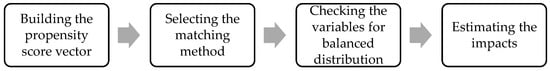
Figure 2.
Diagram of the Propensity Score Matching procedure.
Two approaches to determining the growth rate were considered. The first one consisted of using the geometric mean of chain indexes and would actually mean taking the initial and final datapoints of the time series into consideration. However, that approach was found to be poorly substantiated, especially as the processes studied did not follow a steady (upward or downward) trend. As shown by a preliminary analysis of empirical data, the growth rates of the phenomena concerned did not always follow a clear trend. As a consequence, in order to determine the growth rate, the authors used an approach which was based on all datapoints of the time series and, thus took into account the diverse changes throughout the study period. Following this, the average growth rate served as a basis for determining the dynamics of selected farm variables in both groups in the period t0–t5, as per the formula below [65]
where
- n: the number of years considered when determining the dynamics of the phenomenon;
- m: n (n-1);
- yt: the value of the phenomenon in the years considered.
3. Results and Discussion
3.1. Results of the Propensity Score Matching Procedure
Propensity Score Matching was performed in STATA 15 with the use of the psmatch2 command. The one-to-one closest neighbor matching procedure was used: exactly one unit of the control group was attributed to each unit of the beneficiary group. It was decided to use a unified matching technique for all countries in order to increase the comparability of results. An attempt was made to use other techniques in order to improve the matching quality for Lithuania and Latvia, but this did not fundamentally change the differences between the control pool and the beneficiary group in these countries, and had an adverse effect on the quality of matching in other countries. Considering the absence of statistical significance, the results for these two countries were not interpreted in further detail. Because the common option was checked, beneficiaries with a pscore above the maximum or below the minimum level for the control group were excluded from the matching procedure. This allowed us to reject considerable outliers. The results of matching, including the average values of variables before and after matching, percentage errors, error reduction and statistical significance tests are as shown in Table 2, Table 3 and Table 4. In summary, the PSM method allowed us to create two groups (the beneficiaries and the control group) for each country (except Latvia and Lithuania). As they do not significantly differ in average indicators (of labor, land and capital), they are statistically identical.
Table 2.
Results of the matching procedure for the variable “labor” (in AWU, SE010).
Table 3.
Results of the matching procedure for the variable “land” (in ha, SE025).
Table 4.
Results of the matching procedure for the variable “capital” (in EUR, SE441-SE446).
3.2. Productive Input Resources Owned by Farms
The first part of the analysis was to examine the changes in productive input resources (Table 5). In accordance with Article 20 of Council Regulation (EC) No. 1698/2005 [66], the support for targeting the competitiveness of the agricultural sector concerns measures aimed at restructuring and developing physical potential and promoting innovation through the modernization of agricultural holdings. This modernization is based on grants for investments in farm machinery and equipment such as tractors, harvesters, farm buildings, manure storage, and irrigation facilities [67]. In accordance with these program assumptions, investment support is expected to result in an increase in fixed asset value. This was the outcome attained in all countries from the group who accessed pro-investment funds. Note that, in all countries (except Slovakia), both the increase in asset value and the pace of changes were higher in the beneficiary group than in the control group. This means that the investment funds available under the second pillar of the CAP clearly provided an investment incentive. In many countries, they actually made development investments possible. This is true for Hungary and Slovenia, where the value of assets held by the control group followed a slight downward trend. In turn, in the Czech Republic and Poland, it remained virtually unchanged. In addition to increasing the value of their fixed assets, farms which accessed investment funds also grew in size. A positive net effect also exists for the area of agricultural land: indeed, the experimental group reported a greater increase in acreage, with Czech Republic as the sole exception. However, the decline in the area of Czech farms can actually be considered negligible, which means that a stagnation was observed, especially as the average farm area was very large (the average area of a Czech beneficiary farm recorded in the FADN was circa 1200 ha). In turn, the comparison of the pace of changes between the area of agricultural land and the value of fixed assets clearly shows that financial support was allocated to enhancing the technical equipment of farms (fixed assets). There are two essential reasons for this: first, in the context of the implementation of investment funds under the CAP, the purchase of land was not considered an eligible cost; moreover, the purchase of land is limited by land availability, irrespective of the financing options (own funds, loan or non-repayable funds disbursed under the agricultural policy), and land investments thus primarily depend on land supply.
Table 5.
Productive input resources in beneficiary farms in the base year (preceding the year where the beneficiaries accessed the pro-investment mechanisms under the second pillar of the CAP) and in the fifth year after they accessed the respective funds.
The resulting substitution of labor with capital is one of the elements assessed as part of the changes driven by the implementation of CAP pro-investment measures. It is an important and expected outcome, especially in countries which continue to struggle with structural problems affecting their agriculture. The findings reveal that an ambiguous direct relationship exists between changes in capital and the decline in farm employment. Furthermore, no clear differences can be identified between the beneficiary group and the control farms in the countries surveyed. The Czech Republic, Estonia, Slovakia and Hungary witnessed a reduction in average employment figures in the five subsequent years following the completion of investments (this was true for both beneficiary and control farms), whereas in other countries average employment levels remained virtually unchanged. These differences between the countries can be explained by two factors: first, not all investments are labor-saving—if the investment was targeted at increasing production volumes (e.g., the construction or extension of animal housings or purchase of land), additional farm employment was needed, and conversely, if the purpose of the investment was to purchase more efficient machinery or equipment, fewer people were required to operate it and perform the work—second, the purchase of technologically sophisticated equipment could require the farm to employ specialists. Whatever the reasons may be, note that these are specific situations which differ between farms, whereas FADN data—at such a high degree of generality—do not allow for a case-by-case analysis. However, even if this was possible, it still would not provide a clear general answer. This was confirmed by Nilsson [25], who noted that the operators “can receive different levels of subsidies depending on the nature of the investment project and the characteristics and choice of the firm, which may affect the outcome”.
3.3. Productivity and Profitability of Farms
As part of the defined research tasks, the authors also sought to trace the changes in productivity (Table 6) and profitability (Table 7) of productive inputs used in beneficiary farms (compared to the control group). Characteristically, in most countries, beneficiary farms had a higher productivity and profitability for all productive inputs in the year preceding access to funds (t0) than the control group. Significant differences in this respect were discovered for land productivity and profitability in the Czech Republic; labor productivity and profitability in Estonia; labor profitability in Hungary; and productivity and profitability of all productive inputs (except for capital profitability) in Slovenia. Poland was an exception; in the initial period, all productivity ratios were significantly higher in the control group, whereas land and capital profitability was significantly higher in beneficiary farms. The PSM routine was based on productive input resources (in the year preceding access to support funds, t0). Hence, the conclusion from the comparison is that the beneficiaries of investment funds disbursed under the second pillar of the CAP were farms at a (slightly) higher or similar level of the productivity and profitability of inputs. In a dynamic approach (starting from the year preceding access to support funds, and moving through the five subsequent years), it appears that, in beneficiary farms, the increase in fixed asset values was faster than the changes in production value; only in Poland and Slovenia did production value per euro of fixed assets grow at an average annual rate of 3% and 4.5%, respectively. In these two countries and in the Czech Republic, changes in fixed capital profitability followed a similar trend, i.e., growth was recorded in the first two years upon completing the investment. Irrespective of the (growth or decline) trends followed by capital profitability, farms from the control group demonstrated better performance (faster growth or slower decline, respectively). In the 5th year of the analysis, statistically significant differences in capital productivity and profitability (testifying to the advantage of the control group) were found in all countries except Czech Republic and Slovakia. This is understandable in the context of the consequences of the investments which, as mentioned earlier, increase fixed capital value much faster in farms which access investment funds. When estimating the net effect of changes in the productivity and profitability of fixed capital (the difference in the pace of changes between the beneficiary and control group), it seems that, in all countries, the control group experienced a more advantageous transformation than the beneficiary group. However, it is important to note that the effects of investments (primarily including the increase in production) will come to light only in the long run, which goes beyond the five-year analysis period. This means that farms which access funds under the second pillar of the CAP implement investments that develop their production potential; the resulting improvements in production and income performance are of a rather long-term nature and go beyond the first years following the completion of the investment. These findings are consistent with that noted by Nilsson [25] as regards intervention in the loan market, namely that the support has enabled firms to modernize their holdings and realize investments with new production techniques, which in turn improved their productivity. However, in the case of CAP funds, the improvements in productivity and profitability are long-term effects.
Table 6.
Productivity of productive input (measured as total output) of beneficiary farms which accessed pro-investment funds under the second pillar of the CAP and of control farms in the base year (preceding the year where the beneficiaries accessed the pro-investment mechanisms under the second pillar of the CAP) and in the fifth year after they accessed the respective funds.
Table 7.
Profitability of productive input (measured as Gross Farm Income) of beneficiary farms which accessed pro-investment funds under the second pillar of the CAP and of control farms in the base year (preceding the year where the beneficiaries accessed the pro-investment mechanisms under the second pillar of the CAP) and in the fifth year after they accessed the respective funds.
Indeed, land productivity and profitability increased in beneficiary farms, even though they increased their area of agricultural land. The pace of this process was comparable to changes in productivity in the control group (Poland, Slovenia), whether slower (Estonia, Hungary) or slightly faster (Czech Republic). When considering all the countries covered by this study, the beneficiary group has no obvious advantage over the control group in terms of changes in land productivity and profitability (a statistically significant positive net effect was recorded for land productivity and profitability in Slovenia). As with the case of capital productivity, this could be explained by differences in investment types. However, a general conclusion can be drawn that, while no clear positive net effect exists for land productivity and profitability in all countries, none of the countries saw a deterioration in the situation of beneficiaries (in relation to the control group) during the first 5 years following the investment.
From the perspective of structural changes, and when assessing the implementation effects of CAP pro-investment mechanisms, an important remark is that, in all countries, farms which implemented the program were capable of increasing their labor productivity and profitability, just like the control group. The average annual production growth rate and the growth in income per unit of labor input was clear (from 2.6% in Hungary to as much as 7.5% in Czech Republic. In these countries, as was the case for land, a statistically significant positive net effect (a difference in growth rate between the beneficiary group and the control group) was recorded in Slovenia, but also in Poland, where beneficiary farms reported a greater increment in labor profitability and reduced the negative difference in labor productivity. It is important that, despite the investment, beneficiary farms were able to maintain or increase labor profitability in the first years following the implementation.
4. Conclusions
The purpose of this study was to determine the net effect of implementing pro-investment instruments available under the second pillar of the CAP in selected Central and Eastern European countries. With regard to developing production potential (i.e., the availability of productive inputs), structural funds disbursed under the CAP clearly provided an investment incentive for farms. In many countries, they actually made development investments possible. In addition to increasing the value of their fixed assets, farms which accessed investment funds also expanded their resources of agricultural land. When assessing the changes, it is important to note that most countries saw a positive net effect because the beneficiaries reported a greater increase in fixed asset value and in farm area (except for Slovakian beneficiaries, who experienced a decline in both fixed asset value and land resources, and for Czech beneficiaries, who witnessed a reduction in their land resources). The comparative analysis of countries covered by this study failed to clearly confirm that labor is substituted with capital to a significant extent.
Regarding the productivity and profitability of productive inputs, the characteristic finding is that in the year preceding access to funds (t0), the results recorded by beneficiary farms were slightly better than, or comparable to, what was found in the control group. This is true for all countries except Poland, where the control group had significantly better levels of all productivity ratios in the initial period, while beneficiary farms had higher levels of land and capital profitability. Therefore, the beneficiaries of investment funds disbursed under the second pillar of the CAP were farms at a (slightly) higher or similar level of productivity of inputs. It is important to note, however, that the countries covered by this study differed in the observed net effects of investment mechanisms implemented. Every country covered by this study experienced a noticeable negative net effect on both the productivity and profitability of capital. In the 5th year of the analysis, statistically significant differences in capital productivity and profitability (testifying to the advantage of the control group) were found in all countries except Czech Republic and Slovakia. Although beneficiary farms had higher capital growth rates than the control group, they were not accompanied by a pro-rated increase in output value and income. When considering all the countries, the beneficiary group has no clear advantage over the control group in terms of changes in land productivity and profitability (a statistically significant positive effect was recorded for land productivity and profitability in Slovenia). This was similar for labor: a statistically significant positive net effect (a difference in growth rate between the beneficiary group and the control group) was recorded in Slovenia, but also in Poland where beneficiary farms reported a greater increment in labor profitability and reduced the negative difference in labor productivity. Beneficiary farms were able to maintain or increase labor profitability in the first years following the implementation of the investment. In can be reasonably expected (knowing the particularities of agricultural investments) that farms which access funds under the second pillar of the CAP implement diverse investments that develop their production potential; the outcomes (improvements in productivity and profitability) will emerge in different periods, often in the long term, which goes beyond the first years following the completion of the investment.
This study can provide guidelines for CAP decision makers, especially in the context of the new EU financial perspective for 2021–2027. The differences in the net effects of pro-investment measures between the countries suggest that subsidies should be aligned as much as possible with the characteristics of the local agricultural sector, which undoubtedly determine the outcomes of intervention mechanisms. As a consequence, the allocated funds will be used as efficiently as possible, resulting in the improved effectiveness, quality and cohesion of programs implemented. Furthermore, taking into account the long-term rate of return on agricultural investments could also provide some guidelines for agricultural policy regarding investment support mechanisms. Due to the particularities of agricultural production, farm investments are of a long-term nature (the buildings, constructions, machinery and equipment have a years-long lifecycle). Considering the above, it may be expected (though caution must be exercised) that the outcomes of investments, depending on their type, will also come to light with different delays, which will often be longer than the initial years following the completion of the investment. If the above hypothesis can be deemed true, it is worth considering whether the application documents related to investment support mechanisms should require the beneficiaries to outline the expected outcomes of investments over a longer period (e.g., a ten-year period).
Keeping the above in mind, the authors intend to extend the analysis period by several years in their further research. This will allow us to carry out more in-depth research on the impact of investments on economic sustainability, which is often attained as a long-term outcome. Moreover, it seems useful to carry out a similar analysis which, rather than considering all the farms together, would focus on representatives of the same type of farming or farms with a similar acreage and to make an attempt to determine the impact of the investment type on how fast the outcomes emerge.
Author Contributions
Conceptualization, W.C. and K.P.P.; methodology, W.C. and K.P.P.; software, W.C. and K.P.P.; validation, W.C. and K.P.P.; formal analysis, W.C. and K.P.P.; investigation, W.C. and K.P.P.; resources, W.C. and K.P.P.; data curation, W.C. and K.P.P.; writing—original draft preparation, W.C. and K.P.P.; writing—review and editing, W.C. and K.P.P.; visualization, W.C. and K.P.P.; supervision, W.C. and K.P.P.; project administration, W.C. and K.P.P.; funding acquisition, W.C. and K.P.P. All authors have read and agreed to the published version of the manuscript.
Funding
This research was funded by National Science Centre, Poland, grant number UMO-2018/31/N/HS4/03052.
Acknowledgments
Data source: EU-FADN – DG AGRI.
Conflicts of Interest
The authors declare no conflict of interest.
References
- Boone, L.; Dewulf, J.; Ruysschaert, G.; D’Hose, T.; Muylle, H.; Roldán-Ruiz, I.; Van linden, V. Assessing the consequences of policy measures on long-term agricultural productivity—Quantification for Flanders. J. Clean. Product. 2020, 246, 1–10. [Google Scholar] [CrossRef]
- Dong, F.X.; Mitchell, P.D.; Colquhoun, J. Measuring farm sustainability using data envelope analysis with principal components: The case of Wisconsin cranberry. J. Environ. Manag. 2015, 147, 175–183. [Google Scholar] [CrossRef] [PubMed]
- Savickiene, J.; Miceikiene, A. Sustainable economic development assessment model for family farms. Agric. Econ. Czech 2018, 64, 527–535. [Google Scholar] [CrossRef]
- Gafsi, M.; Legagneux, B.; Nguyen, G.; Robina, P. Towards sustainable farming systems: Effectiveness and deficiency of the French procedure of sustainable agriculture. Agric. Syst. 2006, 90, 226–242. [Google Scholar] [CrossRef]
- Gliessman, S.R. Agroecology: The Ecology of Sustainable Food Systems; CRC Press: Boca Raton, FL, USA, 2007. [Google Scholar]
- Lazíková, J.; Lazíková, Z.; Takáč, I.; Rumanovská, Ľ.; Bandlerová, A. Technical efficiency in the agricultural business—The case of slovakia. Sustainability 2019, 11, 5589. [Google Scholar] [CrossRef]
- De Koeijer, T.J.; Wossink, G.A.A.; Struik, P.C.; Renkema, J.A. Measuring agricultural sustainability in terms of eficiency: The case of Dutch sugar beet growers. J. Environ. Manag. 2002, 66, 9–17. [Google Scholar] [CrossRef]
- Zolin, M.B.; Pastore, A.; Mazzarolo, M. Common agricultural policy and sustainable management of areas with natural handicaps. The veneto region case study. Environ. Dev. Sustain. 2019, 1–19. [Google Scholar] [CrossRef]
- Himics, M.; Fellmann, T.; Barreiro-Hurle, J. Setting climate action as the priority for the common agricultural policy: A simulation experiment. J. Agric. Econ. 2020, 71, 50–69. [Google Scholar] [CrossRef]
- Runowski, H. The problem of assessing the level of agricultural income in European Union. Ann. Pol. Assoc. Agric. Agribus. Econ. 2017, 19, 185–190. [Google Scholar]
- Hergrenes, A.; Berknel, H.; Linem, G. Income instability among farm households—Evidence from norwey. farm management. J. Inst. Agric. Manag. 2001, 11, 37–48. [Google Scholar]
- Samuelson, P.A.; Nordhaus, W.D. Ekonomia (Economics); Rebis Press: Poznań, Poland, 2012. [Google Scholar]
- Zawalińska, K.; Majewski, E.; Wąs, A. Long-term changes in the incomes of the Polish agriculture compared to the European Union. Ann. Pol. Assoc. Agric. Agribus. Econ. 2017, 17, 346–354. [Google Scholar]
- Kutkowska, B. Support of agricultural incomes by direct payments in farms located in the lower silesia area. J. Agribus. Rural Dev. 2009, 2, 101–109. [Google Scholar]
- Poczta-Wajda, A. Polityka Wspierania Rolnictwa a Problem Deprywacji Dochodów Rolników w Krajach o Rożnym Poziomie Rozwoju (Agricultural Support Policy and the Problem of Income Deprivation for Farmers in Countries with Different Levels of Development); PWN Press: Warsaw, Poland, 2017. [Google Scholar]
- Czubak, W. Rozwój Rolnictwa w Polsce z Wykorzystaniem Wybranych Mechanizmów Wspólnej Polityki Rolnej Unii Europejskiej (Development of Agriculture in Poland Using Selected Mechanisms of the Common Agricultural Policy of the European Union); Publishing House of the Poznań University of Life Sciences: Poznań, Poland, 2013. [Google Scholar]
- Czubak, W.; Sadowski, A. The priorities of rural development in EU countries in years 2007–2013. Agric. Econ. Czech 2013, 59, 58–73. [Google Scholar]
- Swinnen, J.F.M.; Gow, H.R. Agricultural credit problems and policies during the transition to a market economy in central and Eastern Europe. Food Policy 1999, 24, 21–47. [Google Scholar] [CrossRef]
- Lerman, Z. Reform and farm restructuring in central and eastern Europe: A regional overview. In Structural Change in the Farming Sectors in Central and Eastern Europe; Technical Paper 465; Csaki, C., Lerman, Z., Eds.; World Bank: Washington, DC, USA, 2000; pp. 39–65. [Google Scholar]
- Swinnen, J. Major trends and developments in the agribusiness and agricultural sectors in CEE and NIS. In Proceedings of the EBRD/FAO Conference on “Investment in Agribusiness and Agriculture in CEE and the CIS”, Budapest, Hungary, 20–21 March 2002. [Google Scholar]
- Frohberg, K. Competitiveness of Farming in Countries Associated with the EU under the Common Agricultural Policy. In Structural Change in the Farming Sectors in Central and Eastern Europe; Technical Paper 465; Csaki, C., Lerman, Z., Eds.; World Bank: Washington, DC, USA, 2000; pp. 39–65. [Google Scholar]
- Sarris, A.; Doucha, T.; Mathijs, E. Agricultural Restructuring in Central and Eastern Europe: Implications for Restructuring and Rural Development. Eur. Rev. Agric. Econ. 1999, 26, 305–330. [Google Scholar] [CrossRef]
- Sin, A.; Nowak, C. Comparative analysis of EAFRD’s measure 121 (“Modernization of agricultural holdings”) implementation in Romania and Poland. Procedia Econ. Financ. 2014, 8, 678–682. [Google Scholar] [CrossRef]
- Medonos, T.; Ratinger, T.; Hruška, M.; Špička, J. The Assessment of the effects of investment support measures of the rural development programmes: The case of the Czech Republic. J. Agris Line Papers Econ. Inform. 2012, 4, 35–47. [Google Scholar]
- Nilsson, P. Productivity effects of CAP investment support: Evidence from Sweden using matched panel data. Land Use Policy 2017, 66, 172–182. [Google Scholar] [CrossRef]
- Czubak, W. Wykorzystanie funduszy Unii Europejskiej wspierających inwestycje w gospodarstwach rolnych (Use of European agricultural fund supporting investments in agricultural holdings in Poland). J. Agribus. Rural Dev. 2012, 3, 57–67. [Google Scholar]
- Bakucs, L.Z.; Latruffe, L.; Fertõ, I.; Fogarasi, J. The impact of EU accession on farms’ technical efficiency in Hungary. Post-Communist Econ. 2010, 22, 165–175. [Google Scholar] [CrossRef]
- Wilkin, J. Ekonomia polityczna reform Wspólnej Polityki Rolnej (he political economics of the Common Agricultural Policy reform). Gospodarka Narodowa (Natl. Econ.) 2009, 229, 1–25. [Google Scholar] [CrossRef]
- Stiglitz, J.E. Incentives, organizational structures, and contractual choice in the reform of socialist agriculture. In The Agricultural Transition in Central and Eastern Europe and the Former U.S.S.R.; Braverman, A., Brooks, K.M., Csaki, C., Eds.; The World Bank: Washington, DC, USA, 1993; pp. 27–46. [Google Scholar]
- Sckokai, P.; Moro, D. Modelling the impact of the CAP Single Farm Payment on farm investment and output. Eur. Rev. Agric. Econ. 2009, 36, 395–423. [Google Scholar] [CrossRef]
- Blancard, S.; Boussemart, J.-P.; Briec, W.; Kerstens, K. Short and long-run credit constraints in French agriculture: A directional distance function framework using expenditure-constrained profit functions. Am. J. Agric. Econ. 2006, 88, 351–364. [Google Scholar] [CrossRef]
- Barry, P.J.; Robison, L.J. Agricultural Finance: Credit, Credit Constraints, and Consequences. In Handbook of Agricultural Economics; Gardner, B., Rausser, G., Eds.; Elsevier: Amsterdam, The Netherlands, 2001; Volume 1, pp. 513–571. [Google Scholar]
- Rosochatecká, E.; Tomšík, K.; Žídková, D. Selected problems of capital assets of Czech agriculture. Agric. Econ. 2008, 54, 108–116. [Google Scholar]
- Guastella, G.; Moro, D.; Sckokai, P.; Veneziani, M. Investment behaviour of EU arable crop farms in selected EU countries and the impact of policy reforms. In Factor Markets; Working Papers, No 42; Centre for European Policy Studies: Brussels, Belgium, 2013. [Google Scholar]
- Czubak, W.; Sadowski, A. Impact of the EU funds supporting farm modernisation on the changes of the assets in Polish farms (Impact of the EU Funds Supporting Farm Modernisation on the Changes of the Assets in Polish Farms). J. Agribus. Rural Dev. 2014, 32, 45–57. [Google Scholar]
- Czubak, W. Nakłady inwestycyjne w rolnictwie polskim w kontekście wdrażania Wspólnej Polityki Rolnej Unii Europejskiej (Investment expenditures in Polish agriculture in the context of the implementation of the Common Agricultural Policy of the European Union). In Problemy Rozwoju Rolnictwa i Gospodarki Żywnościowej w Pierwszej Dekadzie Członkostwa POLSKI w Unii Europejskiej (Problems of Agriculture and Food Economy Development in the First Decade of Poland’s Membership in the European Union); Czyżewski, A., Klepacki, B., Eds.; Publishing House of the Polish Economic Society: Warsaw, Poland, 2015. [Google Scholar]
- Pawłowski, K.P.; Czubak, W. Identification of ways of implementing the 2nd pillar of the CAP in Central and Eastern Europe countries. Zeszyty Naukowe Szkoły Głównej Gospodarstwa Wiejskiego. Ekonomika i Organizacja Gospodarki Żywnościowej (Sci. Noteb. Wars. Univ. Life Sci. Econ. Food Econ. Organ.) 2018, 124, 109–123. [Google Scholar]
- Matthews, A. The Future of Direct Payments. Research for AGRI Committee—CAP Reform Post-2020—Challenges in Agriculture, IP/B/AGRI/CEI/2015-70/0/C5/SC1, Directorate General for Internal Policies, Policy Department B: Structural and Cohesion Policies; European Parliament: Brussels, Belgium, 2016. [Google Scholar]
- Farrell, M.J. The Measurement of Productive Efficiency. J. R. Stat. Soc. Ser. A (Gen.) 1957, 120, 253–290. [Google Scholar] [CrossRef]
- Bonfiglio, A.; Henke, R.; Pierangeli, F.; Pupo D’Andrea, M.R. Effects of redistributing policy support on farmers’ technical efficiency. Agric. Econ. 2019, 51, 305–320. [Google Scholar] [CrossRef]
- Minviel, J.J.; Latruffe, L. Effect of public subsidies on farm technical efficiency: A metaanalysis of empirical results. Appl. Econ. 2017, 49, 213–226. [Google Scholar] [CrossRef]
- Kazukauskas, A.; Newman, C.; Sauer, J. The impact of decoupled subsidies on productivity in agriculture: A cross-country analysis using microdata. Agric. Econ. 2014, 45, 327–336. [Google Scholar] [CrossRef]
- Martinez Cillero, M.; Thorne, F.; Wallace, M.; Breen, J.; Hennessy, T. The Effects of Direct Payments on Technical Efficiency of Irish Beef Farms: A Stochastic Frontier Analysis. J. Agric. Econ. 2018, 69, 669–687. [Google Scholar] [CrossRef]
- Rizov, M.; Pokrivcak, J.; Ciaian, P. CAP Subsidies and Productivity of the EU Farms. J. Agric. Econ. 2013, 64, 537–557. [Google Scholar] [CrossRef]
- Garrone, M.; Emmers, D.; Lee, H.; Olper, A.; Swinnen, J. Subsidies and agricultural productivity in the EU. Agric. Econ. 2019, 50, 803–817. [Google Scholar] [CrossRef]
- Latruffe, L.; Desjeux, Y. Common Agricultural Policy support, technical efficiency and productivity change in French agriculture. Rev. Agric. Food Environ. Stud. 2016, 97, 15–28. [Google Scholar] [CrossRef]
- Boulanger, P.; Philippidis, G. The EU budget battle: Assessing the trade and welfare impacts of CAP budgetary reform. Food Policy 2015, 51, 119–130. [Google Scholar] [CrossRef]
- Dudu, H.; Kristkova, Z. Impact of CAP Pillar II Payments on Agricultural Productivity; JRC Technical Report 106591; Publications Office of the European Union: Luxembourg, 2017. [Google Scholar]
- Michalek, J. Counterfactual Impact Evaluation of EU Rural Development Programmes—Propensity Score Matching Methodology Applied to Selected EU Member States. 1: A Micro-Level Approach; Publications Office of the European Union: Luxembourg, 2012. [Google Scholar]
- Baráth, L.; Fertő, I.; Bojnec, Š. Are farms in less favored areas less efficient? Agric. Econ. 2018, 49, 3–12. [Google Scholar] [CrossRef]
- Grzelak, A. Ocena procesów inwestycyjnych w rolnictwie w Polsce w latach 2000-2011 (Evaluation of investment processes in agriculture in Poland in 2000–2011). J. Agribus. Rural Dev. 2013, 28, 111–120. [Google Scholar]
- Olejniczak, K. Teoretyczne podstawy ewaluacji ex-post (Theoretical foundations of ex-post evaluation). In Ewaluacja Ex-Post. Teoria i Praktyka Badawcza (Ex-Post Evaluation. Research Theory and Practice); Haber, A., Ed.; Polish Agency for Enterprise Development: Warsaw, Poland, 2007; pp. 15–41. [Google Scholar]
- Pufahl, A.; Weiss, C.R. Evaluating the effects of farm programmes: Results from propensity score matching. Eur. Rev. Agric. Econ. 2009, 36, 79–101. [Google Scholar] [CrossRef]
- Winship, C.; Morgan, S.L. The estimation of causal effects from observational data. Annu. Rev. Sociol. 1999, 25, 659–706. [Google Scholar] [CrossRef]
- Strawiński, P. Propensity Score Matching. Własności Małopróbkowe (Propensity Score Matching. Small Sample Properties); Publishing House of the Warsaw University: Warsaw, Poland, 2014. [Google Scholar]
- Kirchweger, S.; Kantelhardt, J. Improving Farm Competitiveness through Farm-Investment Support: A Propensity Score Matching Approach. Paper Presented at the 131st EAAE Seminar in Prague. 2012. Available online: http://ageconsearch.umn.edu/handle/135791 (accessed on 5 January 2020).
- Pawłowska, A.; Bocian, M. Estymacja Wpływu Polityki Rolnej Na Wydajność Pracy z Wykorzystaniem Propensity Score Matching (Estimation the Impact of Agricultural Policy on Labor Productivity Using Propensity Score Matching); Institute of Agriculture and Food Economics-National Research Institute: Warsaw, Poland, 2017. [Google Scholar]
- Rosenbaum, P.R.; Rubin, D.B. The central role of the propensity score in observational studies for causal effects. Biometrika 1983, 70, 41–55. [Google Scholar] [CrossRef]
- Guo, S.; Fraser, M.W. Propensity Score Analysis. Statistical Methods and Applications, 2nd ed.; SAGE Publications INC: Thousand Oaks, CA, USA, 2015. [Google Scholar]
- Trzciński, R. Wykorzystanie Techniki Propensity Score Matching w Badaniach Ewaluacyjnych (The Use of Propensity Score Matching in Evaluation Studies); Polish Agency for Enterprise Development: Warsaw, Poland, 2009. [Google Scholar]
- Rubin, D.B. Matched Sampling for Causal Effects; Cambrige University Press: New York, NY, USA, 2006. [Google Scholar]
- Heckman, J.J.; Ichimura, H.; Todd, P. Matching as an Econometric Evaluation Estimator: Evidence from Evaluating a Job Training Program. Rev. Econ. Stud. 1977, 64, 605–654. [Google Scholar] [CrossRef]
- Holland, P.W. Statistics and causal inference. J. Am. Stat. Assoc. 1986, 81, 945–960. [Google Scholar] [CrossRef]
- Konarski, R.; Kotnarowski, M. Zastosowanie metody propensity score matching w ewaluacji ex-post (Application of the propensity score matching method in ex-post evaluation). In Ewaluacja Ex-Post. Teoria i Praktyka Badawcza (Ex-Post Evaluation. Research Theory and Practice); Haber, A., Ed.; Polish Agency for Enterprise Development: Warsaw, Poland, 2007; pp. 156–183. [Google Scholar]
- Wysocki, F. Metody Taksonomiczne w Rozpoznawaniu Typów Ekonomicznych Rolnictwa i Obszarów Wiejskich (Taxonomic Methods in the Identification of Economic Types of Agriculture and Rural Areas); Publishing House of the Poznań University of Life Sciences: Poznan, Poland, 2010. [Google Scholar]
- Council Regulation (EC). No. 1698. Support for Rural Development by the European Agricultural Fund for Rural Development (EAFRD). Official Journal of the European Union. Available online: http://eur-lex.europa.eu/legal-content/EN/TXT/HTML/?uri=CELEX:32005R1698&from=en (accessed on 10 December 2019).
- Caruso, D.; Contò, F.; Skulskis, V. The implementation of measure 121 of the rural development program: Comparative analysis between Italy and Lithuania. Intellect. Econ. 2016, 9, 102–107. [Google Scholar] [CrossRef]


© 2020 by the authors. Licensee MDPI, Basel, Switzerland. This article is an open access article distributed under the terms and conditions of the Creative Commons Attribution (CC BY) license (http://creativecommons.org/licenses/by/4.0/).