Abstract
A sensitivity analysis is critical for determining the relative importance of model parameters to their influence on the simulated outputs from a process-based model. In this study, a sensitivity analysis for the SPACSYS model, first published in Ecological Modelling (Wu, et al., 2007), was conducted with respect to changes in 61 input parameters and their influence on 27 output variables. Parameter sensitivity was conducted in a ‘one at a time’ manner and objectively assessed through a single statistical diagnostic (normalized root mean square deviation) which ranked parameters according to their influence of each output variable in turn. A winter wheat field experiment provided the case study data. Two sets of weather elements to represent different climatic conditions and four different soil types were specified, where results indicated little influence on these specifications for the identification of the most sensitive parameters. Soil conditions and management were found to affect the ranking of parameter sensitivities more strongly than weather conditions for the selected outputs. Parameters related to drainage were strongly influential for simulations of soil water dynamics, yield and biomass of wheat, runoff, and leaching from soil during individual and consecutive growing years. Wheat yield and biomass simulations were sensitive to the ‘ammonium immobilised fraction’ parameter that related to soil mineralization and immobilisation. Simulations of CO2 release from the soil and soil nutrient pool changes were most sensitive to external nutrient inputs and the process of denitrification, mineralization, and decomposition. This study provides important evidence of which SPACSYS parameters require the most care in their specification. Moving forward, this evidence can help direct efficient sampling and lab analyses for increased accuracy of such parameters. Results provide a useful reference for model users on which parameters are most influential for different simulation goals, which in turn provides better informed decision making for farmers and government policy alike.
Keywords:
sensitivity analysis; winter wheat; drainage; yield; soil water dynamics; soil loss; soil pool 1. Introduction
Process-based models for agricultural systems provide a widely used and efficient tool for understanding the complex interactions between soil water, carbon (C), nitrogen (N), phosphorus (P), and plant growth [1,2], where both production under various environmental conditions [3] and nutrient cycling [4] can be simulated. To run a simulation successfully, models need to be informed with parameters that accurately quantify individual processes, together with local soil conditions, weather, and management practices. However, parameters that might vary with environmental conditions and have varying, possibly complex distributions themselves [5] are often difficult to precisely characterise, especially if they are costly to measure, requiring long-term monitoring [6]. In turn, this parameter variability, uncertainty, or quality directly affects the reliability of the model simulations [1,7]. In general, agricultural simulation models require a large amount of input data and parameters, many of which are difficult to source or collect. At the same time, it is common for only a few parameters to strongly influence (and maximize) the variability of model outputs, while the majority of parameters only provide a weak influence in this respect [8]. Therefore, understanding the likely influence of each parameter on a model’s outputs is crucial, as this allows the number of parameters to be safely reduced without a worrying loss of model accuracy, while at the same time, focus can be placed on data collection for parameters that most strongly influence model performance.
To identify how parameters impact model outputs, sensitivity diagnostics can be calculated through running multiple model simulations while varying the parameters across specific ranges [9]. Sensitivity analysis for model parameterization and outputs have been applied to various cropping systems, soil types and climate conditions using a range of models. For example, Specka et al. [10] applied a parameter sensitivity analysis for modelling above-ground biomass with regard to a future model calibration and an improved understanding of model response patterns; Jabloun et al. [11] assessed the sensitivity of outputs (crop yield and N leaching) from a crop simulation model, where 128 parameters were assessed. A sensitivity analysis quantifies those parameters which are most influential on model outputs, and in this respect can guide the efforts towards improving their accuracy as well as the model’s output accuracy [12].
The SPACSYS model is implemented in a modular approach and provides a field-scale and weather-driven dynamic process-based simulation model of water, C and N cycling between plants, soils, and microbes [13]. The model has been widely used to assess the impact of climate change [14,15,16], tillage [17], fertilizer application [16,18], and different cultivars [19] on agricultural systems in terms of crop yields, C and N budgets, soil physical properties, and soil water redistribution. However, the model requires over 200 parameters for the simulation of various processes and plant growth and development. It would therefore be informative and beneficial to assess which parameters the SPACSYS outputs are the most and the least sensitive to, so that there can be guidelines for its use when all 200 parameters are not readily available.
A sensitivity analysis has also been used in building and understanding the structure of agro-ecosystem models [20,21]. Distinctions are made between a local and global sensitivity analysis (LSA and GSA, respectively), where the former is also known as a ‘one at a time’ (OAT) approach, while the latter considers multiple parameters at the same time. Thus, an LSA does not consider any interactions between parameters, while a GSA does. Both GSA [22] and LSA [23,24,25,26] have merit, where in ideal situations both should be applied and their results objectively assessed and compared [27,28]. In studies where uncertainty and interactions in model parameters are minimal, then an LSA may suffice [27] over the inherently more complex, GSA. Specifically, Link et al. [27] concludes that an LSA may suffice for situations where the ranking of model parameters is of importance, while GSA should be used for a precise attribution of variance in model outputs. Of course, it should be noted that results and insights from literature are always dependent on the characteristics of the process-based models employed.
Given this study is the first to identify parameter input sensitivity for the SPACSYS model, we chose to present results in two stages: first, an LSA as presented here, and second, a GSA (which is prep.) for presentation elsewhere. This two-stage reporting approach is followed for computational reasons, together with differences in associated interpretations, visualisations, and comparisons of the LSA and GSA outputs. Given SPACSYS requires over 200 parameters, assessing and reporting the sensitivity of them all would be problematic, for both an LSA and a GSA alike. Further, different subsets of parameters would be chosen according to their likely importance in simulating different processes under different background conditions. Because of computational and associated interpretation constraints, an LSA can investigate the sensitivity of outputs to a greater number of input parameters and investigate the distribution of each input parameter more intensively, than that feasible with a GSA. A GSA for, say, only four parameters entails the added investigation of six 2-parameter interactions, four 3-parameter interactions, and one 4-parameter interaction, which themselves vary on how the parameter input distributions are described (likely done simply, with say low, medium, and high values only). Given these thorny design and implementation issues for a GSA, for this study, we only consider the effects of a single parameter change on outputs via an LSA. This allows for a greater number of parameters to be investigated coupled with more detailed descriptions of the parameter distributions than would be viable within a GSA.
For this study, we carried out an LSA on the parameters that control soil water redistribution, and C and N cycling with the SPACSYS model, using a winter wheat field experiment conducted at Rothamsted Research in Harpenden, UK as the case study. To investigate potential influences of climatic and soil conditions on the analysis, simulations with the same configurations were run with different climatic and soil conditions. The study objectives were: (1) to identify those parameters that have the maximum influence on the simulation outputs with respect to wheat production and environment risks under UK soils and climatic conditions, and (2) to examine and understand the relationships between parameter sensitivity and model outputs.
2. Materials and Methods
2.1. Study Site
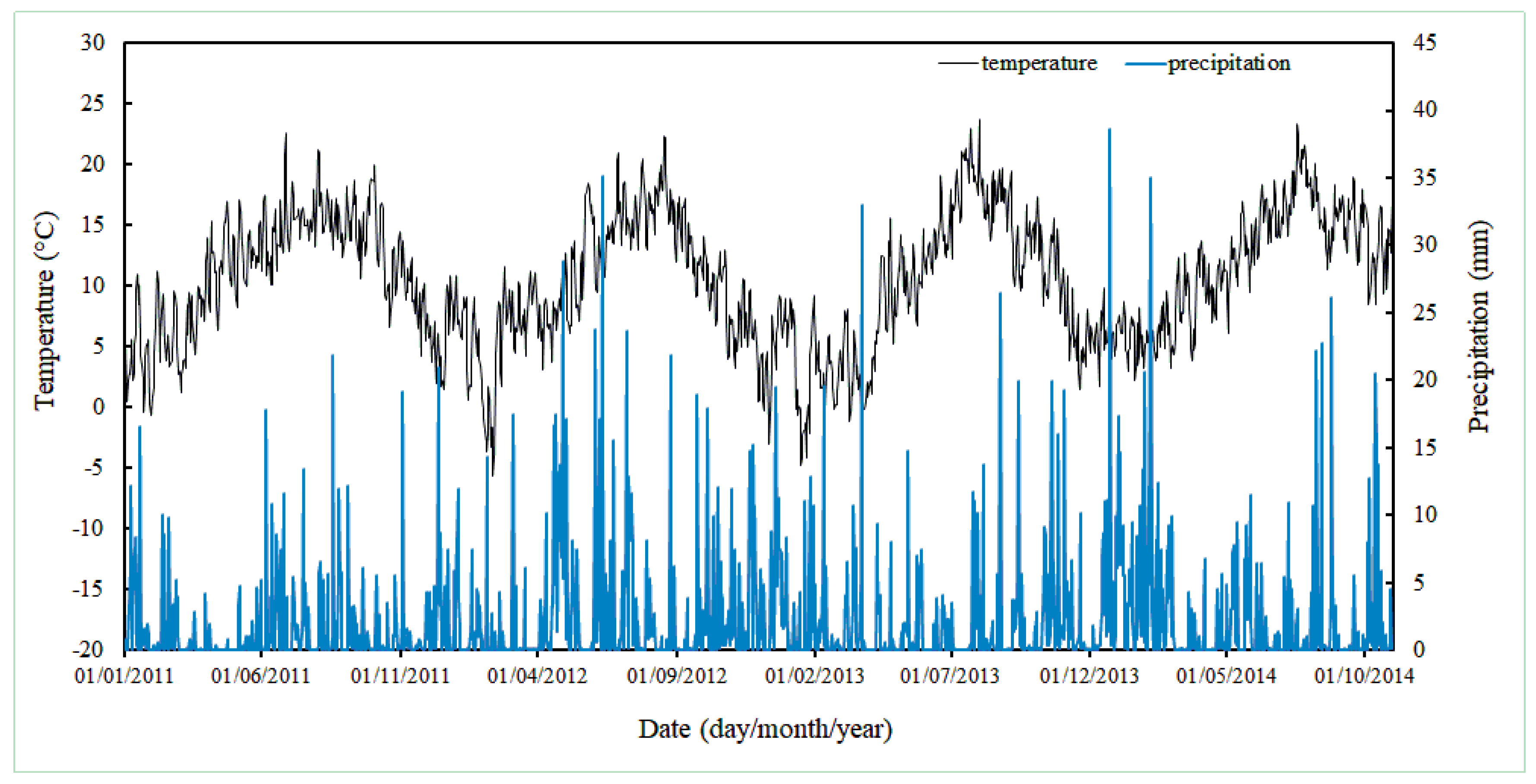
Data from a winter wheat field experiment was used for this study. The experiment was conducted for three growing seasons from 2011 to 2014 in the experimental plots of “Exhaustion Land”, one of the classical long-term experiments at Rothamsted Research in Harpenden (51°49′ N, 0°21′ W and 128 m a.s.l.). The winter wheat cultivar was Xi-19. The soil is classified as a Chromic Luvisol (FAO classification) with a silty clay loam texture topsoil. Daily maximum and minimum air temperatures and precipitation during the growing years are shown in Figure 1. Compared to the mean climatic conditions over the growing season between 1981 and 2010 (mean temperature is 8.7 °C, precipitation 611mm), the first growing season and the third growing season were warmer and wetter (9.4 °C and 770 mm, 10.1 °C and 814 mm, respectively), but the second season was cooler and dryer (7.9 °C and 672 mm, respectively). The total sunshine hours of the three growing seasons (1314, 1268, and 1363 h, respectively) were all higher than the 1981 to 2010 mean (1243 h). Data for the study period were downloaded from the electronic Rothamsted Archive (e-RA, http://www.era.rothamsted.ac.uk/, accessed on 30 June 2021).
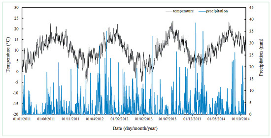
Figure 1.
Daily rainfall and mean air temperature over the observational period (2011 to 2014).
2.2. Parameters and Simulated Outputs
A total of 61 model required parameters, describing both water redistribution and C and N processes, were chosen to investigate the responses of the system. To reduce complexity in the analysis, parameters that relate to crop growth and development were set as the usual default values, and thus not part of the 61 parameters investigated. The ranges (maximum to minimum) of the chosen parameters were ± 50% of the default values used in previous studies [29,30,31]. Each parameter was set to one of 100 different values to ensure sampling points are uniformly distributed across the probability distribution. A total number of 6100 SPACSYS simulations were run, each with a 3-years length, meaning that only one of 61 parameters (Table A1) was investigated in turn, whilst all others were set at their default. Details on the linkage of each parameter to each process can be found in various applied SPACSYS model studies [13,32] and also in subsequent, developmental studies [31].
For the simulation outputs, a total of 27 variables were considered. Variables include those for grain yield and above-ground dry matter biomass of winter wheat, soil water dynamics, losses (runoff, leaching, and release) from soil and nutrient pool sizes (Table A2).
2.3. Sensitivity Analysis and Diagnostics
As indicated above, only the effect of a single parameter change on the simulated outputs was considered—i.e., an LSA was followed. We analysed sensitivity to the 61 parameters by ranking the values of the root mean square deviation (RMSD) of simulated outputs as follows:
where D represents the simulated value using the default parameter values (Wu, et al., 2019) and Si represents the simulated values as defined above, at the ith step of parameter changes and n is equal to 100 (the number of simulations). In order to ensure that all results from the SPACSYS runs, with each of 61 parameters varying in turn, can be assessed and objectively compered to each other, we used the normalized RMSD (NRMSD) as follows:
where Smax is the maximum value of all the simulated outputs for the whole set (100 simulations) of a single parameter over the entire simulated period. The NRMSD diagnostic combines RMSD values across multiple output variables to produce an overall measure of model sensitivity, while normalising for the different scales of the outputs. It can be interpreted as a fraction of the maximum values. The higher the NRMSD, the more sensitive the output variables are to the given parameter specification. A parameter that yields an NRMSD equal to 0% means it contributes very little on the simulated outputs and can be taken as a fixed parameter [33]. Simulations are considered sensitive to parameters yielding NRMSD values > 1%.
In order to capture the effects of different weather conditions on parameter sensitivity, we calculated the NRMSD in each individual growing year (2011/12, 12/2013, and 13/2014) and consecutive years (2011/13, 12/2014, and 11/2014). Further clarity was provided with averaged NRMSDs for the individual growing years and consecutive years:
where NRMSDIN and NRMSDCD represent the averaged NRMSD for the individual and the consecutive years, respectively. NRMSD1, NRMSD2, NRMSD3, NRMSD12, NRMSD23, and NRMSD123 represent the NRMSD for years 2011/12, 2012/13, 2013/14, 2011/13, 2012/14, and 2011/14, respectively. All analyses were carried out within the R statistical programming environment (version 3.5.0).
2.4. Simulated Climate and Soil Data
In order to assess the impact of climate and soil type on the results of the sensitivity analysis, four additional simulation runs were built with the same configuration as the main simulation experiment described—replacing the weather over the simulation period with another set collected for South West England (50°46′10′′ N, 3°54′05′′ W) and replacing soil properties with (a) a sandy soil with 10% clay, 70% sand, and 20% silt content in the top 10 cm layer, with 12% clay, 72% sand, and 16% silt content in the 10–20 cm layer and with 15% clay, 75% sand, and 10% silt content in the 20–30 cm layer; (b) a loam soil with 20% clay, 40% sand, and 40% silt content in the top 10 cm layer, with 22% clay, 42% sand, and 36% silt content in the 10–20 cm layer and with 25% clay, 45% sand, and 30% silt content in the 20–30 cm layer; and (c) a clay soil with 80% clay, 10% sand, and 10% silt content in the top 10 cm layer, with 76% clay, 12% sand, and 12% silt content in the 10–20 cm layer and with 70% clay, 15% sand, and 15% silt content in the 20–30 cm layer. Additional simulations were configured as described in Section 2.2, where the use of default parameter values was considered reasonable.
3. Results
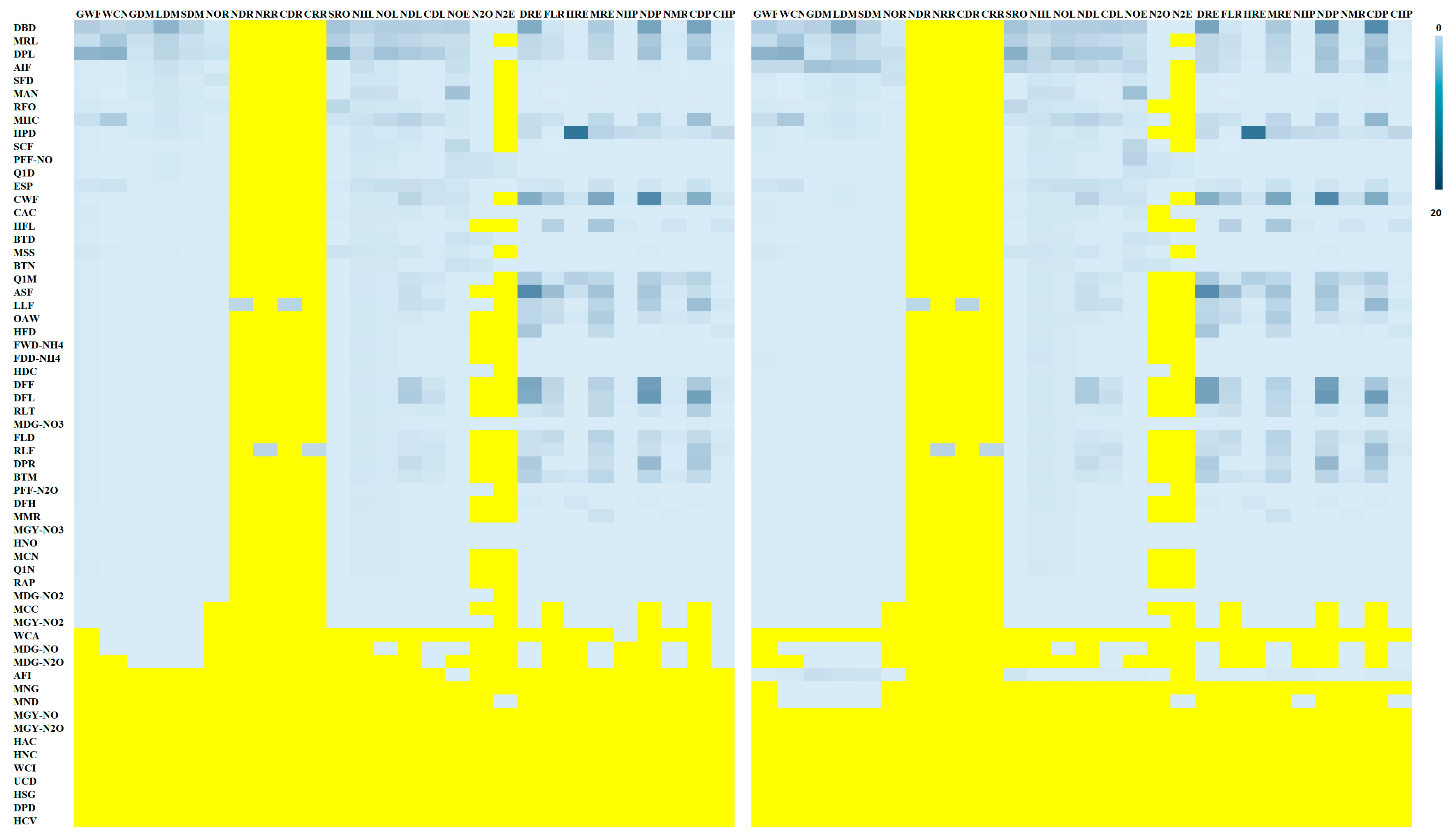
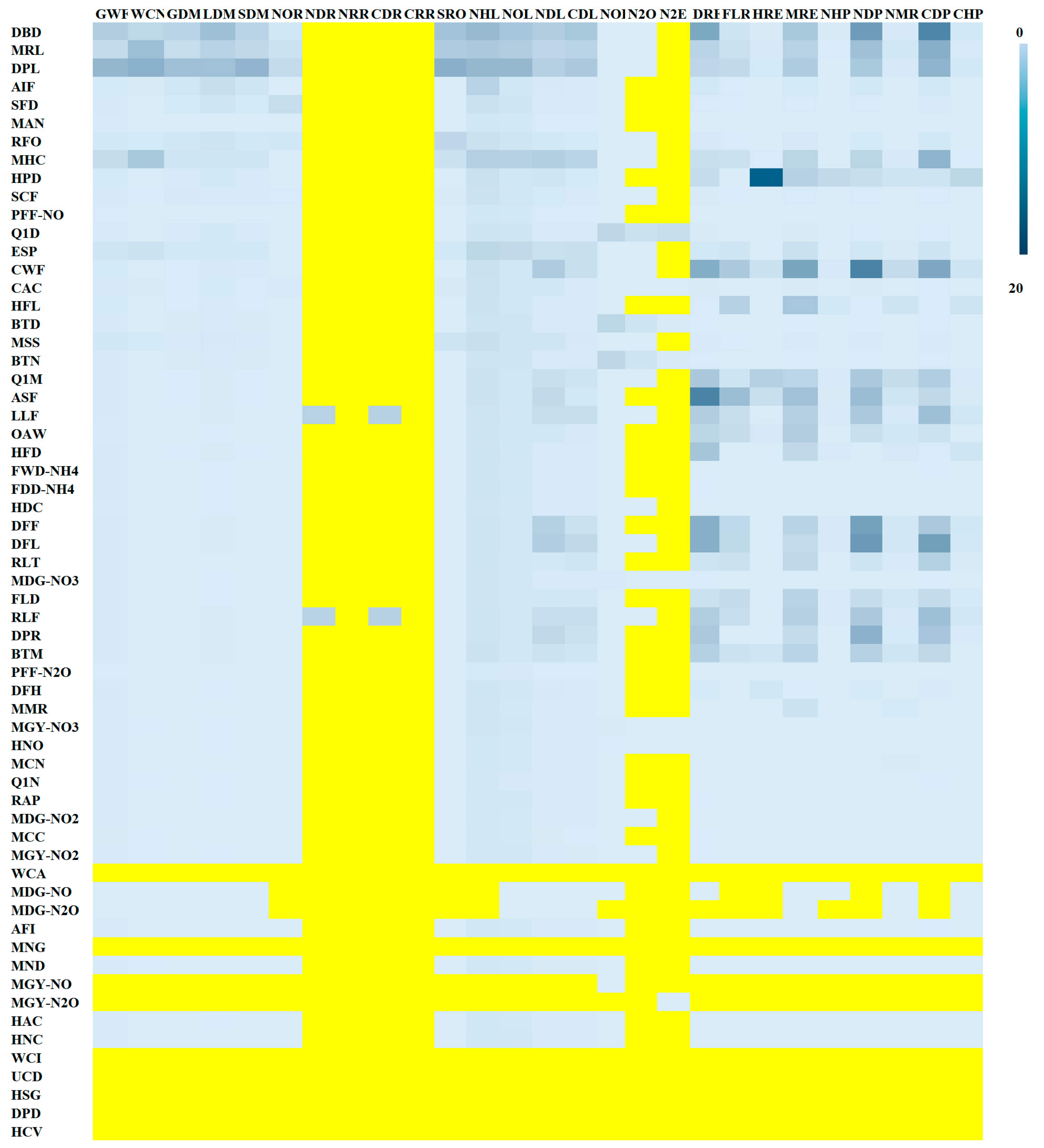
Figure 2 maps the influence of each of the 61 parameters with respect to their effect on the simulations of 27 output variables both for the individual growing years and the consecutive years. The values of NRMSD range between 0 to 16%, with 87.83% between 0 and 1%. Output variables were insensitive to 11 of the 61 parameters, as their NRMSDs were all 0. The 11 parameters were: maximum nitrifier growth rate (MNG), maximum growth yield on NO (MGY-NO), maximum growth yield on N2O (MGY-N2O), half ammonium concentration (HAC), half NOx concentration (HNC), water content interval to unity (WCI), unsaturated conductivity decrease (UCD), half saturation global radiation intensity (HSG), drain pipe diameter (DPD), and finally, half closure vapour pressure deficit (HCV).
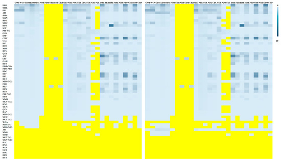
Figure 2.
Heat maps of averaged NRMSDs for the 61 parameters (rows) with respect to the 27 output variables (columns) under the experimental condition from individual years (left) and the pairs of consecutive years (right). A yellow pixel represents no interaction.
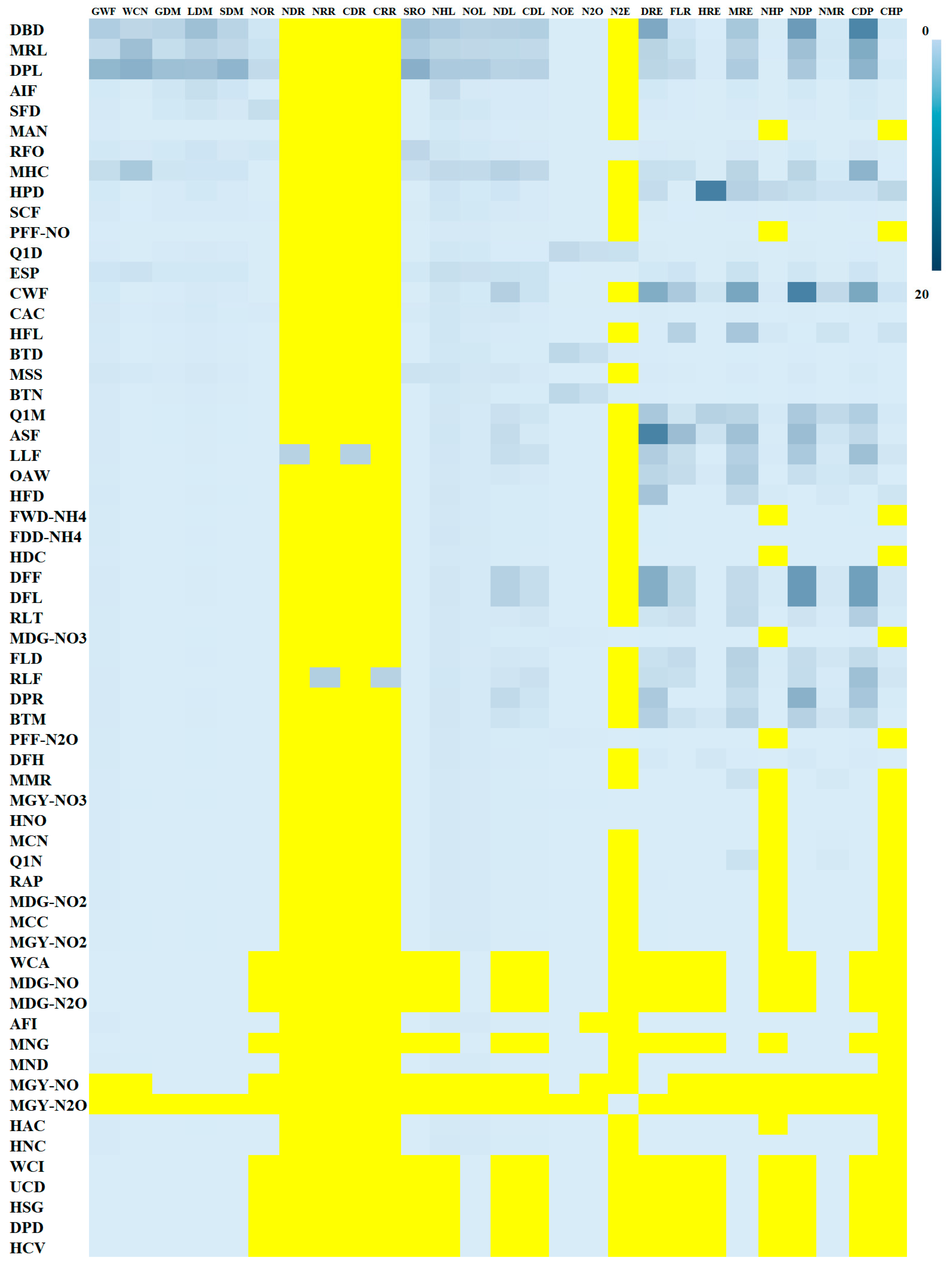
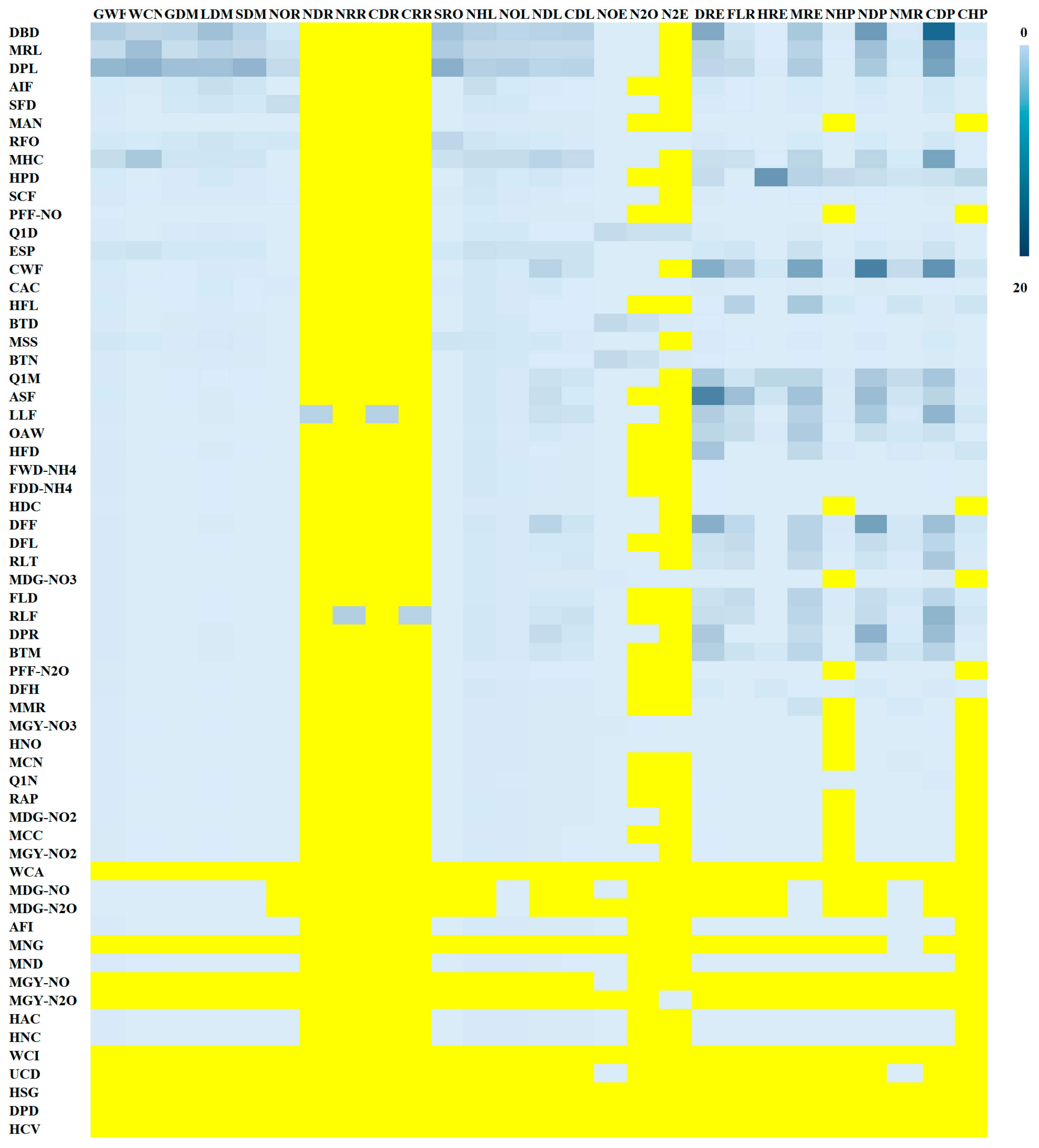
The influences of the parameters on the chosen output variable under alternative weather conditions are shown in Figure 3 and with the three different soil types in Figure 4 (sandy), Figure 5 (loam), and Figure 6 (clay). The results from these additional climate and soil simulations were hardly different to those from the main simulation experiment (Figure 2), where the sensitive parameters with NRMSD greater than 1% were almost identical. However, the number of fixed parameters reduced, especially in the sandy soil where none of the 61 parameters could be taken as fixed.
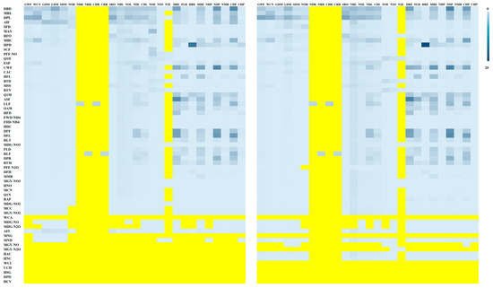
Figure 3.
Heat maps of averaged NRMSDs for the 61 parameters (rows) with respect to the 27 output variables (columns) with the climate condition in South West England from individual years (left) and the pairs of consecutive years (right). A yellow pixel represents no interaction.

Figure 4.
Heat maps of averaged NRMSDs for the 61 parameters (rows) with respect to the 27 output variables (columns) in the sandy soil from consecutive years. A yellow pixel represents no interaction.
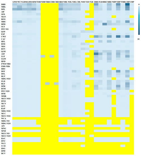
Figure 5.
Heat maps of averaged NRMSDs for the 61 parameters (rows) with respect to the 27 output variables (columns) in the loam soil from consecutive years. A yellow pixel represents no interaction.

Figure 6.
Heat maps of averaged NRMSDs for the 61 parameters (rows) with respect to the 27 output variables (columns) in the clay soil from consecutive years. A yellow pixel represents no interaction.
As the most sensitive parameters had similar trends across all the simulations (main and additional), regardless of climate or soil type, we now focus our attention only on the relationships between the parameters and the output variables from the main simulation experiment. Here the greatest sensitivity to parameter specification was observed for simulated outputs grouped as: (1) soil water dynamics, (2) crop dry matter accumulation, and (3) N and C losses and pools.
3.1. Soil Water Dynamics
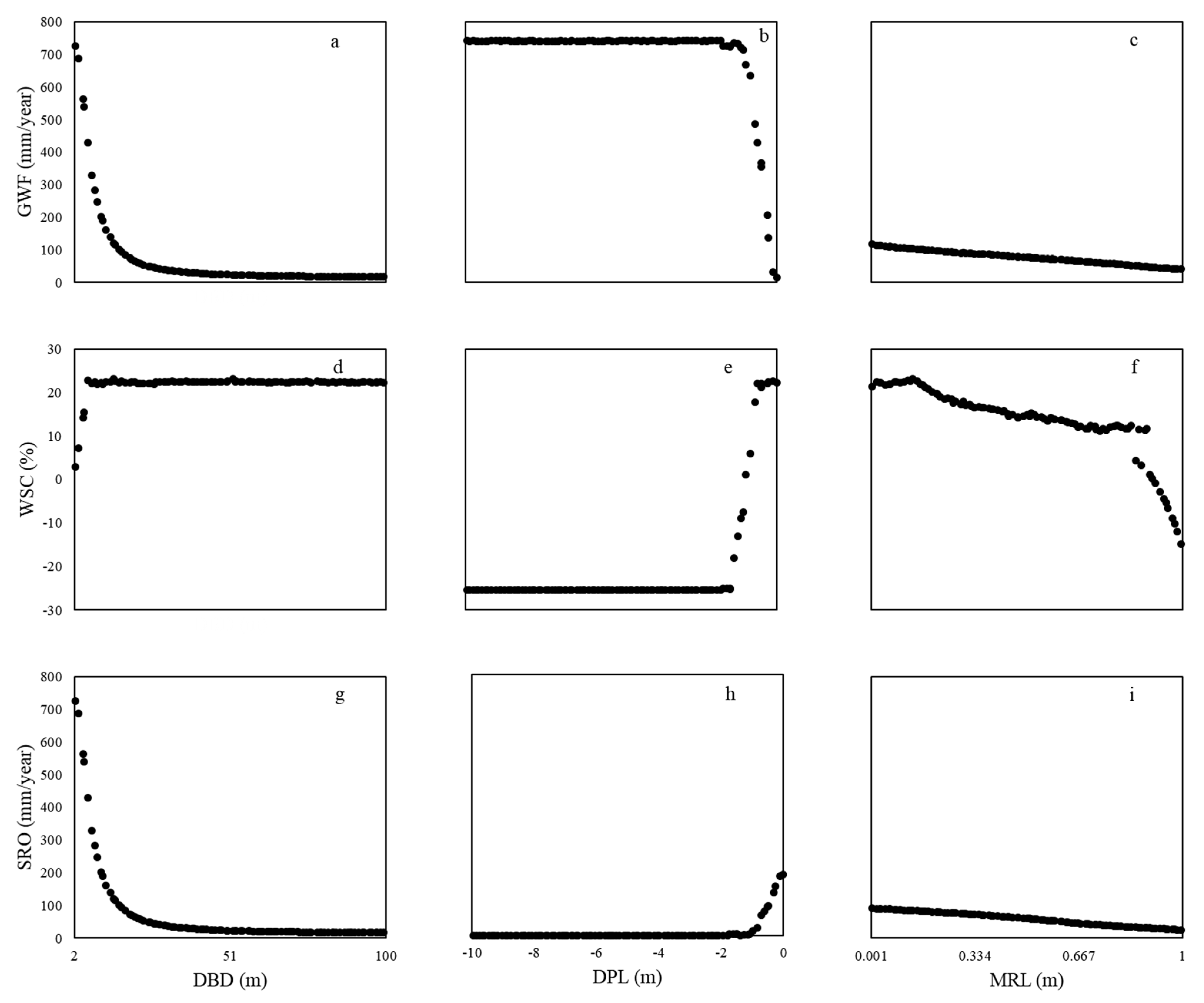
The drainpipe level (DPL) parameter had the greatest influence on the simulations for ground water flow (GWF) and water content change (WSC) with NRMSD values > 7% (Figure 2), especially when the specified value of DPL was from the surface to the 2 m soil depth (Figure 7b,e,h). Here GWF increased and then plateaued at around 2 m, while WSC decreased moving from positive to negative values. For DPL values between 0 and −2 m, surface runoff (SRO) decreased from about 570 mm/year to values of zero. Likewise, other parameters relating to the drainage system, such as distance between drainpipes (DBD) and minimum roughness length (MRL) were similarly influential with NRMSD values > 1% and > 3% (Figure 2) for GWF, WSC, and SRO outputs (Figure 7). Here GWF, WSC, and SRO outputs all decreased as the MRL parameter increased from its minimum (0.001 m) to maximum specification (1 m) (Table A1 in Appendix A), while only GWF and SRO outputs decreased as the DBD parameter increased from its minimum (2 m) to maximum specification (100 m) (Table A1). The influence of minimum hydraulic conductivity (MHC), runoff first order rate coefficient (RFO) and maximum surface storage (MSS) parameters on GWF, WSC, and SRO outputs are given in Figure A1 in Appendix A.
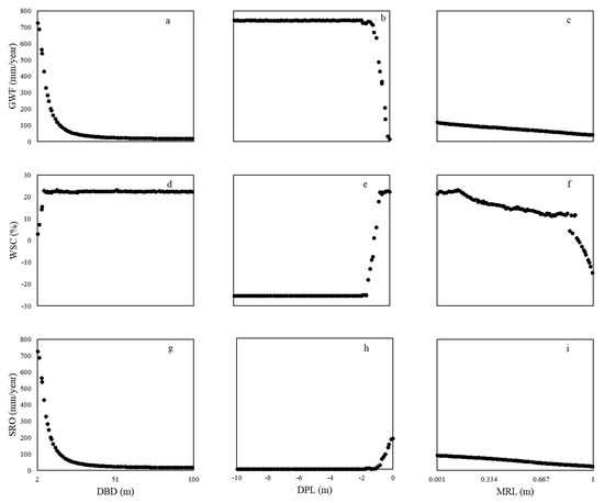
Figure 7.
Response of averaged drainage water fluxes and the change in soil water content change (i.e., groundwater flow (GWF, a–c), water content change (WSC, d–f) and surface runoff (SRO, g–i)) to parameter change for distance between drainpipe (DBD), drain pipe level (DPL), and minimum roughness length (MRL) over the simulation period.
3.2. Dry Matter of Winter Wheat
The simulation of dry matter of leaves, stems, and grains for winter wheat (LDM, SDM, and GDM) are particularly sensitive to parameters DBD, MRL, DPL, and AIF (ammonium immobilisation fraction) following their NRMSD values (Figure 2). DBD was the most sensitive parameter (NRMSD > 3%) for LDM, SDM, and GDM in the individual years, with increases in dry matter simulation only for DBD < 40 m. However, SDM and GDM were most sensitive to AIF with NRMSD > 4%, where dry matter simulation increased slightly across the full range of the AIF values specified (i.e., 0 to 1). Increases in dry matter were found for DPL > −2 m, while a stepped but small increase in dry matter was observed for MRL across its minimum to maximum values specified (Figure A2 in Appendix A).
3.3. Nitrogen and Carbon Losses from Soil
3.3.1. Losses with Surface Runoff
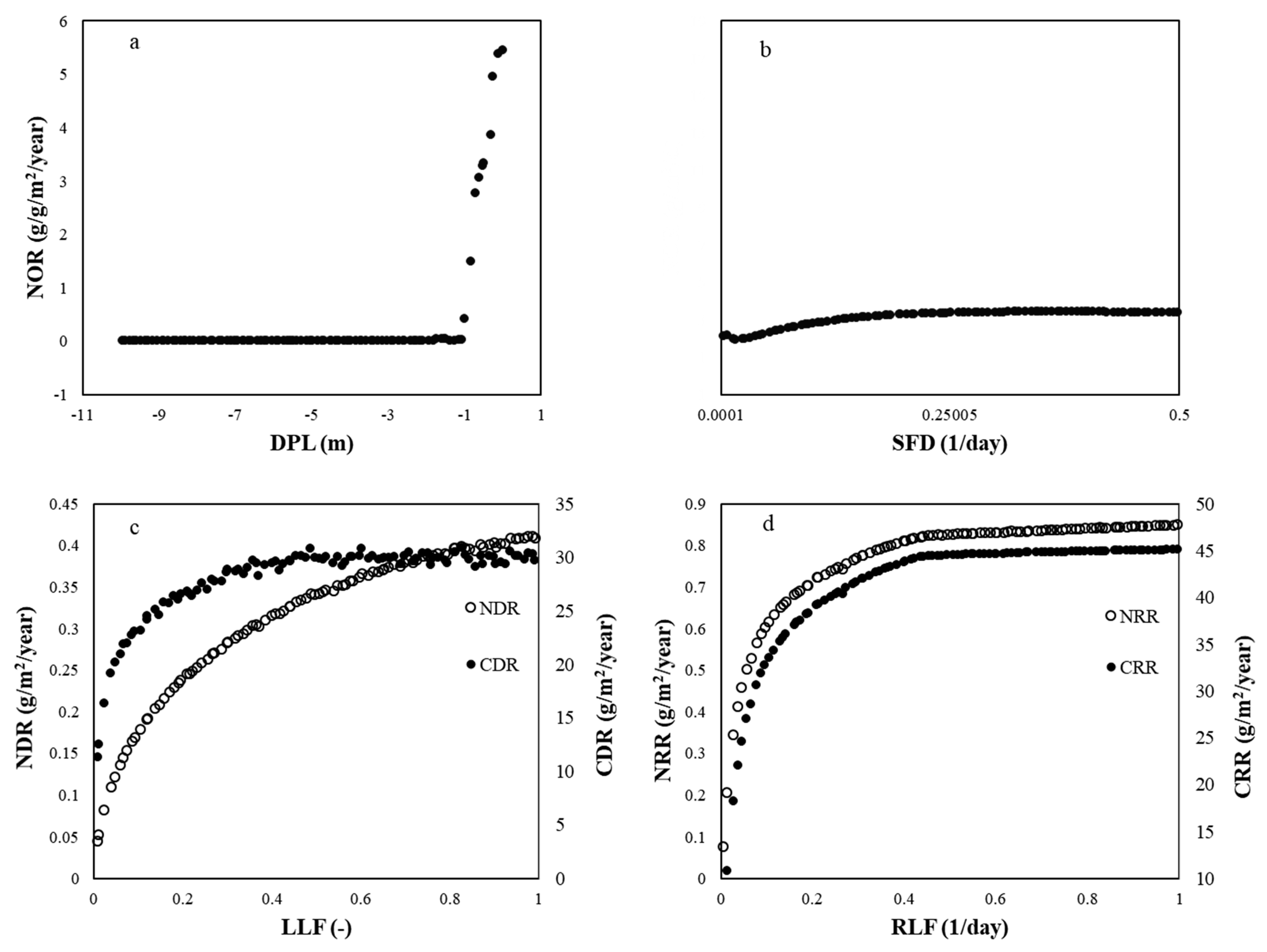
The simulations for nitrate (NO3) loss with surface runoff (NOR) were also highly sensitive to DPL, with NRMSD values of 1.38% and 1.73% in the individual and pairs of consecutive years, respectively (Figure 2). For DPL > −2 m, NOR displayed an increasing trend (Figure 8a). As would be expected, simulations for NOR were also sensitive to the fertiliser dissolution rate (SFD), where NOR simulations displayed a non-linear increase for SFD < 0.2. (Figure 8b). With NRMSD values > 0%, the simulations of dissolved N loss (NDR) and C loss (CDR) with surface runoff were sensitive to the loss of litter parameter (LLF) (Figure 8c), and the simulations of residue N loss (NRR) and residue C loss (CRR) were sensitive to the loss of residue parameter (RLF) (Figure 8d).

Figure 8.
Relationships for simulations of: (a) NO3 runoff (NOR) and parameter drain pipe level (DPL), (b) NOR and parameter specific fertiliser dissolution rate (SFD), (c) dissolved N loss (NDR) and C dissolved loss (CDR) and parameter litter loss (LLF), and (d) residue N loss (NRR) and residue C loss (CRR) and parameter residue loss (RLF) over the simulation period.
3.3.2. Nitrogen and Carbon Leaching
With the specification of parameters DBD, MRL, DPL, MHC, and ESP (the empirical scale in pore shape), each had a clear influence on the simulations of leaching for NO3 (NOL), NH4 (NHL), N (NDL), and C (CDL) in the individual and pairs of consecutive years (Figure 2). The same variable simulations were also sensitive to parameters AIF, LLF, RLF, DFF (a transferring fraction of decomposed fresh litter to dissolved organic matter), DFL (a transferring fraction of litter to dissolved organic matter), CWF (coefficient in the water function for decomposition), and DPR (potential decomposition rate of dissolved organic matter). DBD was a highly influential parameter for NOL and NHL with NRMSDs > 3% whilst DPL was highly influential for NDL and CDL with NRMSDs > 4%. Relationships between output simulations of NOL, NHL, NDL, and CDL and parameters DBD, MRL, DPL, AIF, MHC, ESP, DFF, DFL, CWF, DPR, LLF, and RLF are given in Figure A3 and Figure A4 in Appendix A.
3.3.3. Gas Emissions
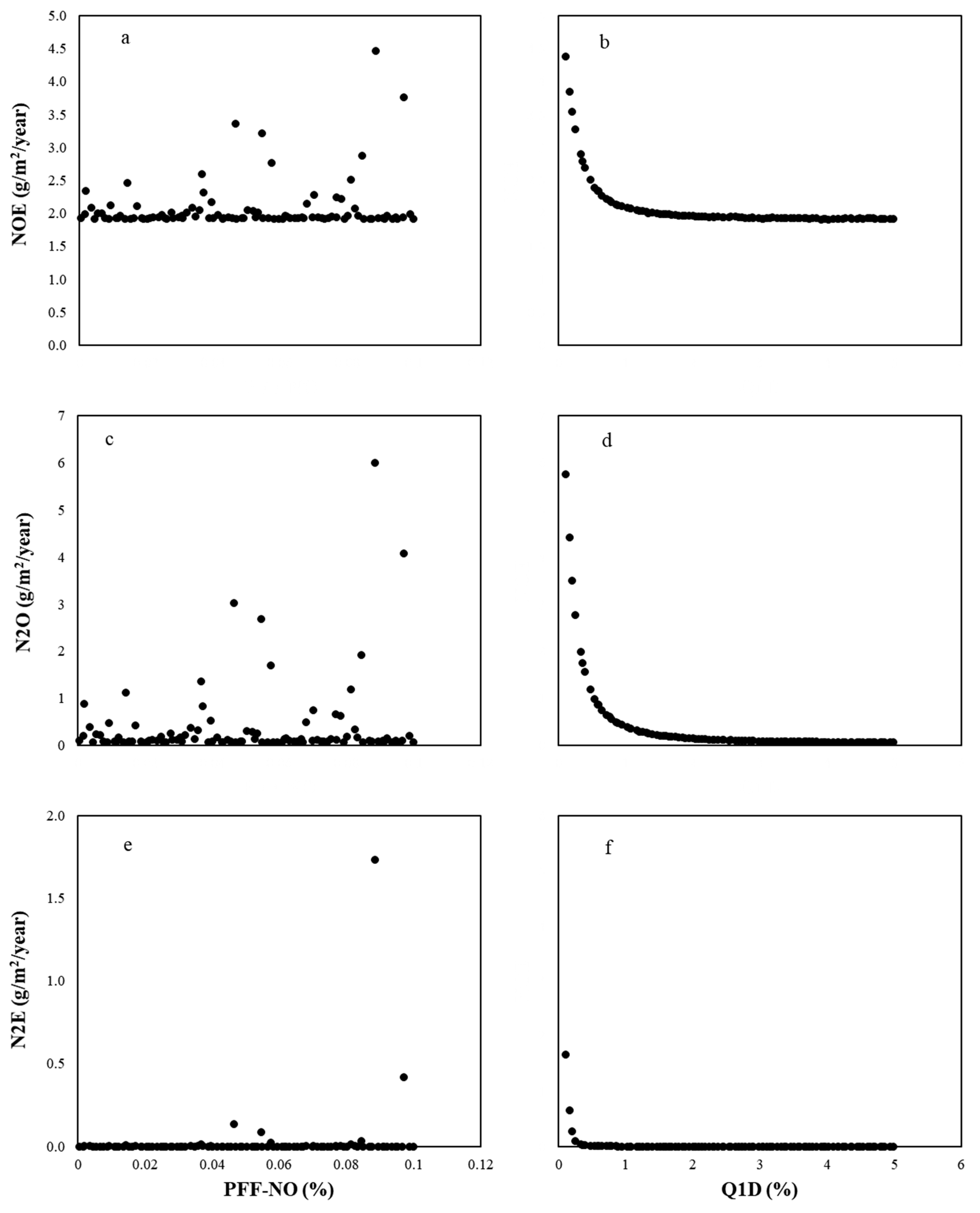
Simulations of the N2O emission rate (N2O) were most sensitive to changes in the maximum autotrophic nitrification rate (MAN), secondly, the NO production fraction from nitrification (PFF-NO), and thirdly, the Q10 temperature coefficient for denitrification (Q1D) (Figure 2). Specification of the latter two parameters also strongly influenced the NO emission rate (NOE) and N2 emission rate (N2E) (Figure 2). In addition, N2O simulations were found to be relatively sensitive to DBD, MRL, and DPL (Figure 2). Figure 9 displays the relationships between the nitrogenous gas emissions outputs (NOE, N2O, and N2E) and a range of values for parameters PFF-NO and Q1D. For the range of PFF-NO specified, the simulation of NOE, N2O, and N2E were erratic with no clear pattern. Further plots for NOE only are given in Figure A5 in Appendix A.
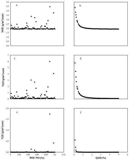
Figure 9.
Relationships between simulations of nitrogenous gas emissions (NOE: NO emission rate (a,b), N2O: N2O emission rate (c,d), and N2E: N2 emission rate (e,f)) and the parameters of NO production fraction from nitrification (PFF-NO) and Q10 value for denitrification (Q1D).
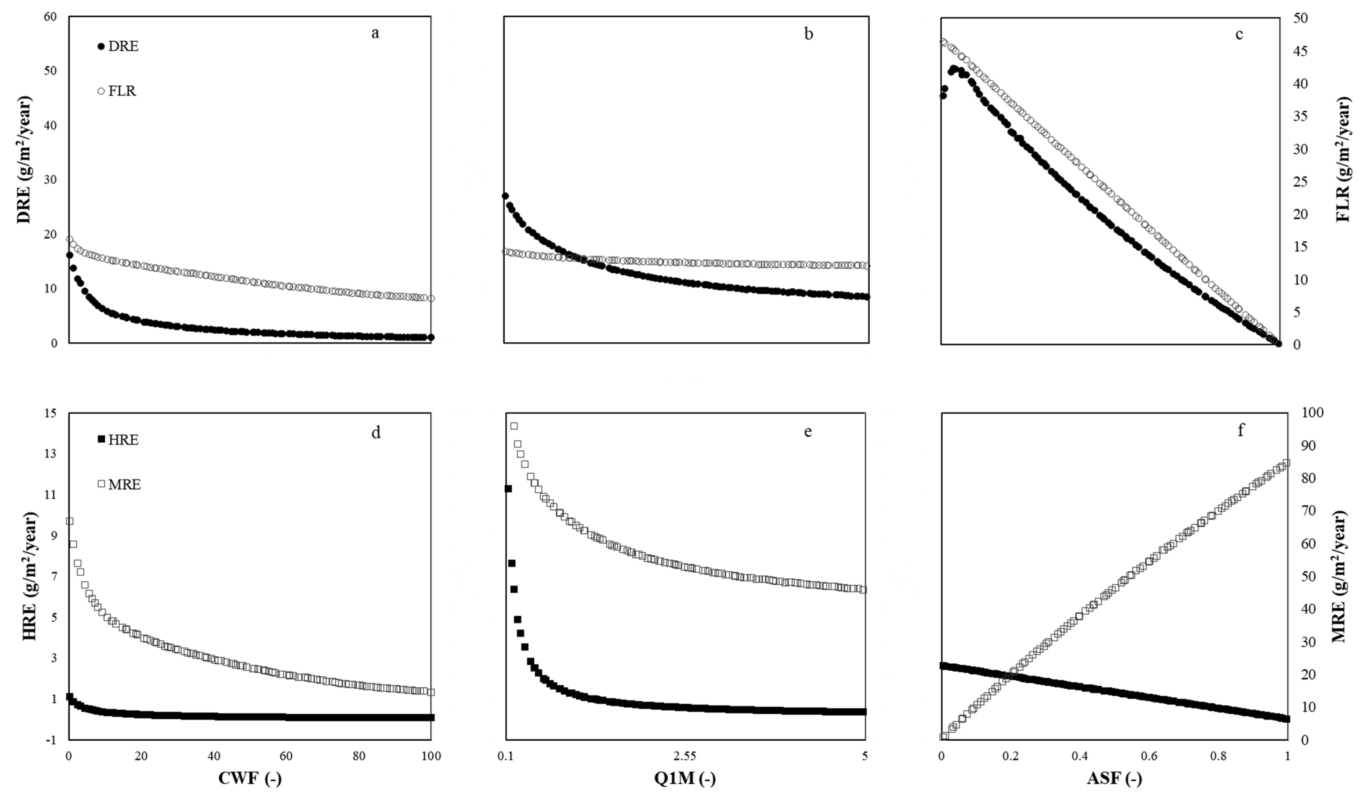
Parameters CWF, Q1M (Q10 temperature coefficient for mineralization), and ASF (assimilation factor), in general, provided the highest NRMSDs (Figure 2) with respect to influencing CO2 emissions from various soil organic C pools (DRE: dissolved release; FLR: fresh litter release; HRE: humus release; MRE: microbial release). However, the simulation of HRE was most sensitive to the humus potential decomposition rate (HPD) (NRMSD > 15%) (Figure 2). Figure 10 displays the relationships between CO2 emissions DRE, FLR, HRE, MRE with respect to the top-ranking sensitive parameters CWF, Q1M, ASF over the simulation period. Almost all CO2 emission outputs deceased as CWF, Q1M, and ASF parameters were increased through their minimum/maximums set (Table A1); the exception being MRE with ASF. Further CO2 emission plots depicting their sensitivity to key parameters are given in Figure A6, Figure A7 and Figure A8 in Appendix A.

Figure 10.
Relationships between simulations of CO2 emissions from soil organic C pools (DRE: dissolved release; FLR: fresh litter release; HRE: humus release; MRE: microbial release) and the parameters they are most sensitive to (CWF: coefficient in water function; Q1M: Q10 value for mineralization; ASF: assimilation factor) over the simulation period. DRE and FLR vs CWF (a), Q1M (b) and ASF (c). HRE and MLR vs CWF (d), Q1M (e) and ASF (f).
3.4. Changes of Soil C and N Pools
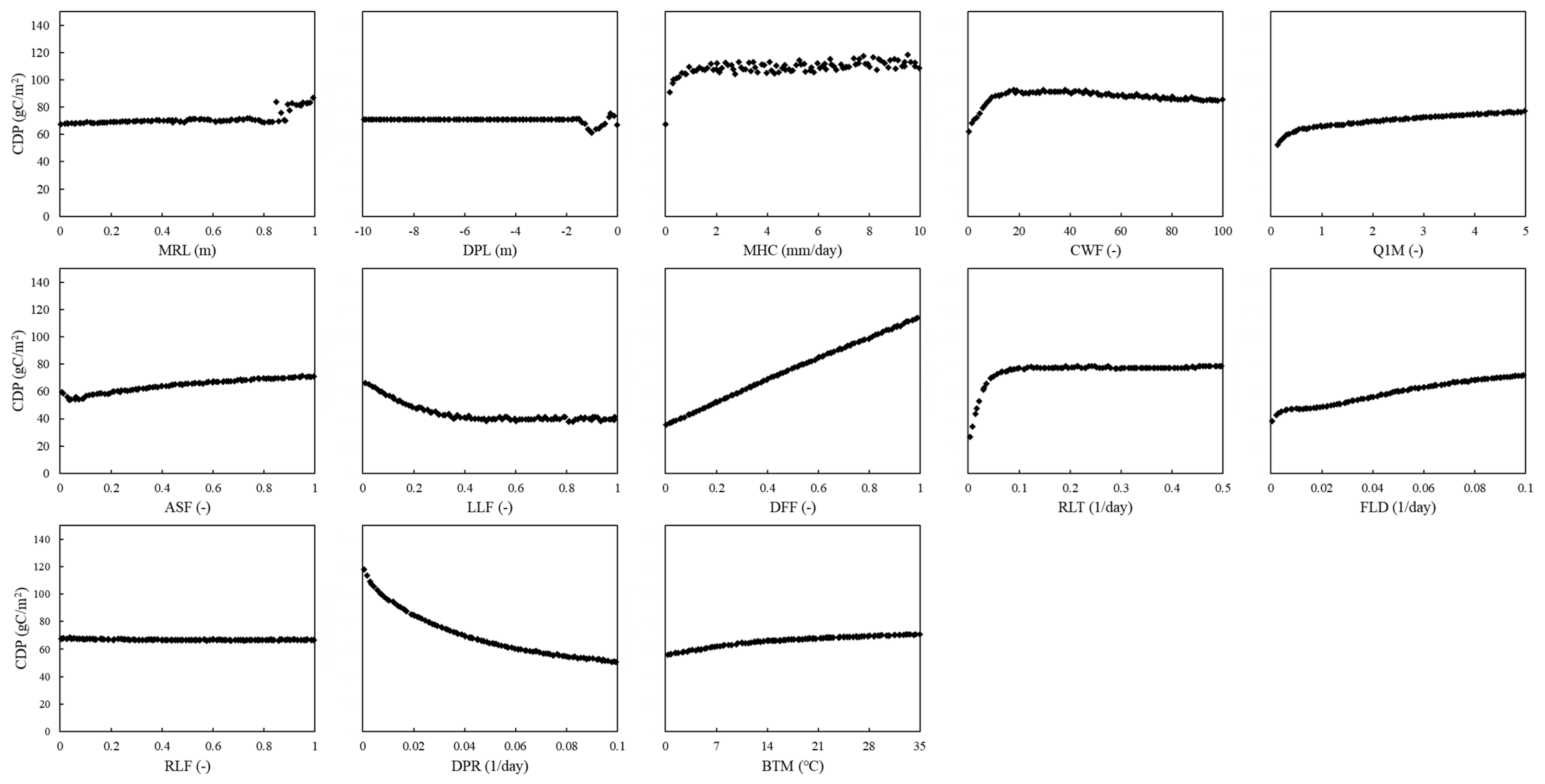
Although simulations of soil N and C pools in humus (NHP and CHP, respectively) were most sensitive to HPD (Figure 2), no discernible trend in this sensitivity was observed (Figure A9a in Appendix A). Simulations of N and C dissolved (NDP and CDP, respectively) were most sensitive to CWF, DFL (dissolved fraction in litter), HFL (humus fraction from fresh litter), and DBD (Figure 2), where in this case, clear increasing trends in this sensitivity were observed, some plateauing (Figure A9b,e for CWF and DBD, respectively), some not (Figure A9c,d for DFL and HFL, respectively). Further soil N and C pools plots depicting their sensitivity to key parameters are given in Figure A10 and Figure A11 in Appendix A.
4. Discussion
Parameters describing drainage implementation (DBD and DPL) play a critical role in the performance of the agriculture system reflecting changes in the weather and soil condition. For this study, simulations for soil water dynamics, crop dry matter accumulation and N and C losses, were all found to be highly sensitive to the specification of DBD and DPL. Our results corroborate with Ballantine and Tanner [34], and Ritzema [35], where both studies demonstrated how the drainage system was an important externality for agricultural production to prevent waterlogging and salinization of the soil in arid and semi-arid regions and strategically control drainage of excess water from the soil profile. It has also been reported that water use efficiency for wheat with a controlled drainage with a varying depth was 40% higher than that with the conventional drainage, depending on the crop stage [36]. Tomic et al. [37] showed that a DBD value of 25 m provided the highest wheat yield among seven different drainage systems, which is in agreement with our result in that DBD is one of the most sensitive parameters for the dry matter of winter wheat. However, this might not be transferrable to other crops, e.g., drainage control was found to have no significant influence on soybean yield [38]. Designing an appropriate drainage system in humid areas can reduce N loss from an agricultural field [39]. By raising the water level in the soil profile, which is equivalent to increasing DPL in our study here, controlled drainage has the potential to increase denitrification in the anaerobic zone [40]. Design of subsurface drainpipes involves the determination of depth (DPL), spacing (DBD) and pipe diameter (DPD) [41]. As a parameter of a drainage system, however, DPD had no influence on any of the 27 selected output variables (Figure 2), which implied the effects of vertical water flow were stronger than horizontal water flow towards the pipes in our study’s wheat field.
Our analysis suggests that simulations were sensitive to changes in MRL (minimum roughness length), where it is known to strongly affect water and heat fluxes on the soil surface [42,43]. Wang et al. [44] have shown that an accurate assessment of soil moisture might be problematic if MRL is inappropriately parameterised. However, our sensitivity analysis showed that SRI, HSG, and HCV (all related to evaporation and transpiration processes, see Table A1) had no influence on any of the 27 selected outputs.
4.1. Sensitive Parameters for Water Dynamics
Soil water dynamics is a key component for nutrient cycling and crop growth and development. Our study showed that soil water dynamics were sensitive to MHC (minimum hydraulic conductivity), DPL, DBD, and MRL (Figure 2 and Figure A1). This is not surprising given that: (1) MHC is a key parameter to control the soil water infiltration process where water moves downward from the surface [45] and (2) soil hydraulic conductivity determines surface energy and water fluxes and then soil water content [46,47,48].
4.2. Sensitive Parameters for Yield and Biomass
For simplicity, we did not include in our sensitivity analysis, the plant biological parameters. Therefore, the identified sensitivities influence biomass accumulation and the grain yield of winter wheat indirectly via other processes. Here DBD, MRL, DPL, and AIF are all important parameters for yield and aboveground biomass simulation (where DBD, MRL, and DPL also influence water dynamics in the soil, as discussed above). Unarguably, soil water content itself plays an important role in yield and aboveground dry matter accumulation under non-irrigation conditions [49,50]. It regulates N cycling and its availability to crops is important, as this in turn, affects crop growth and yield formation [51,52,53]. AIF that can be immobilised when the immobilisation process occurs, impacts crop growth and yield through changing mineralisation, and in sequence, the status of soil N and C content [1,54].
4.3. Sensitive Parameters for Losses from Soil
The drainage parameters DPL and DBD also had significant influence on C and N losses through surface runoff and leaching from soils. In addition, SFD (fertiliser dissolution rate), LLF (loss of litter), and RLF (loss of residue) that are each related to external nutrient inputs also played a critical role in the simulations of surface runoff losses. Results showed that SFD was an influential parameter for the simulations of NHL (NH4 leach); LLF was influential for the simulations of NDR and CDR (dissolved N and C loss); and RLF was influential for the simulations of NRR and CRR (residue N and C loss). External nutrient inputs can increase soil nutrient pools, and in turn, nutrient losses when surface runoff occurs.
Clearly, parameters related to nitrification and denitrification processes have a great influence on nitrogenous gas emissions. A higher nitrification rate increases N availability for the denitrification process that is enhanced by Q1D (Q10 temperature coefficient for denitrification). Specification of MAN (maximum autotrophic nitrification rate) had the biggest influence on NOE (NO emission rate), and both PFF-NO (NO production fraction from nitrification) and Q1D influenced NOE, N2O (N2O emission rate), and N2E (N2 emission rate). Conversely, simulations for soil CO2 release were sensitive to a different set of parameters that control nutrient cycling. Here, the specification for Q1M (Q10 temperature coefficient for mineralization), CWF (coefficient in the water function for decomposition), and ASF (assimilation factor) all had a significant influence on DRE (dissolved release), FLR (fresh litter release), HRE (humus release), and MRE (microbial release) (i.e., outputs variables that generate from decomposition from various soil C pools). Our results are supported by previous studies [55,56,57]. The soil organic matter decomposition rate depends on substrates [58,59], a potential decomposition rate and other abiotic and biotic factors including soil temperature (related to Q1M), soil moisture (i.e., CWF), and microbial activities (i.e., ASF) [60].
5. Conclusions
The local sensitivity analysis for the SPACSYS model using data from a winter wheat field experiment found that parameters related to drainage not only affected drainage fluxes but also grain yield and aboveground dry matter accumulation of winter wheat, and losses of water, C and N from soil under given weather and soil conditions. In addition, parameters related to mineralization and immobilisation processes influenced crop yield and biomass accumulation significantly. Further, parameters that control the nitrification and denitrification processes had a great influence on nitrogenous gas emissions. All results were found to be largely insensitive to different climatic and soil conditions, where identified parameter sensitivity remained relatively the same.
Overall, this study has provided evidence of which parameters require the most care in their specification and in turn, which parameters need to be determined accurately. This evidence can lead to efficient and cost-effective sampling and lab analyses for such parameters. Results provide a reference for model users on which parameters are key for different simulation goals. However, although this study has provided some important advances in model understanding and use, we have only considered the influence of single parameter change at a time on the model outputs. Interaction effects through a global sensitivity analysis were not assessed, and as such, are a focus of current and complementary research.
Author Contributions
Conceptualization, L.W.; methodology, L.W., P.H. and Y.S.; software, L.W.; validation, Y.S.; formal analysis, Y.S.; writing—original draft preparation, Y.S., M.H., P.H. and L.W.; writing—review and editing, Y.S., M.H., P.H. and L.W.; visualization, Y.S. and P.H.; supervision, L.W. All authors have read and agreed to the published version of the manuscript.
Funding
Y.S. was funded by the Chinese Scholarship Council (grant number 201706300103). The research was funded by the BBSRC Institute Strategic Programme (ISP) grant, “Soils to Nutrition” work package 2 grant number BBS/E/C/000I0320.
Institutional Review Board Statement
Not applicable.
Acknowledgments
We thank Andrew Mead for the design of statistical analysis.
Conflicts of Interest
The authors declare no conflict of interest.
Appendix A

Table A1.
List of the parameters chosen for the sensitivity analysis, together with their maximum and minimum units specified.
Table A1.
List of the parameters chosen for the sensitivity analysis, together with their maximum and minimum units specified.
| No. | Abbreviations | Variable Description | Unit | Min | Max |
|---|---|---|---|---|---|
| 1 | SFD | Specific fertiliser dissolution rate | 1/day | 0.0001 | 0.5 |
| 2 | Q1N | Coenzyme Q10 temperature coefficient for nitrification | - | 0.1 | 5 |
| 3 | Q1M | Coenzyme Q10 temperature coefficient for mineralization | - | 0.1 | 5 |
| 4 | Q1D | Coenzyme Q10 temperature coefficient for denitrification | - | 0.1 | 5 |
| 5 | PFF-NO | NO production fraction from nitrification | - | 0.00001 | 0.1 |
| 6 | PFF-N2O | N2O production fraction from nitrification | - | 0.000001 | 0.01 |
| 7 | MHC | Minimum hydraulic conductivity | mm/day | 0 | 10 |
| 8 | MMR | Microbial maintenance respiration rate | 1/day | 0.01 | 2 |
| 9 | MDG-NO3 | Maximum NO3 denitrifier growth rate | 1/day | 1 | 40 |
| 10 | MDG-N2O | Maximum N2O denitrifier growth rate | 1/day | 1 | 20 |
| 11 | MDG-NO2 | Maximum NO2 denitrifier growth rate | 1/day | 1 | 40 |
| 12 | MDG-NO | Maximum NO denitrifier growth rate | 1/day | 1 | 20 |
| 13 | MNG | Maximum nitrifier growth rate | 1/day | 0.1 | 15 |
| 14 | MND | Maximum nitrifier death rate | 1/day | 0.01 | 5 |
| 15 | MGY- NO3 | Maximum growth yield on NO3 | gC/gN | 0.01 | 1 |
| 16 | MGY- NO2 | Maximum growth yield on NO2 | gC/gN | 0.01 | 1 |
| 17 | MGY- NO | Maximum growth yield on NO | gC/gN | 0.01 | 3 |
| 18 | MGY- N2O | Maximum growth yield on N2O | gC/gN | 0.01 | 4 |
| 19 | MAN | Maximum autotrophic nitrification rate | 1/day | 0.001 | 0.1 |
| 20 | MCC | Maintenance coefficient on carbon in denitrification | 1/day | 0.0001 | 0.02 |
| 21 | HPD | Humus potential decomposition rate | 1/day | 0.0000001 | 0.001 |
| 22 | HFL | Partitioning fraction to humus from decomposed fresh litter | - | 0 | 1 |
| 23 | HFD | Partitioning fraction to humus from decomposed dissolved organic matter | - | 0 | 1 |
| 24 | HDC | Michaelis constant on dissolved organic carbon concentration | g/m3 | 1 | 40 |
| 25 | HAC | Michaelis constant on ammonium concentration | gN/m3 | 1 | 30 |
| 26 | HNO | Michaelis constant on NOx concentration | gN/m3 | 50 | 200 |
| 27 | FLD | Fresh litter potential decomposition rate | 1/day | 0.0001 | 0.1 |
| 28 | DBD | distance between drainpipes | m | 2 | 100 |
| 29 | DPR | Potential decomposition rate of dissolved organic matter | 1/day | 0.0001 | 0.1 |
| 30 | UCD | Unsaturated conductivity decrease | - | 0 | 10 |
| 31 | SCF | Soil cover fraction to prevent infiltration | - | 0 | 1 |
| 32 | RFO | Runoff first order rate coefficient | 1/day | 0.01 | 1 |
| 33 | MRL | Minimum roughness length | m | 0.001 | 1 |
| 34 | MSS | Maximum surface storage (no runoff) | mm | 0.01 | 10 |
| 35 | HSG | Half saturation global radiation intensity | J/m2/day | 0 | 10,000,000 |
| 36 | ESP | Empirical scale in pore shape | - | 0.01 | 10 |
| 37 | DPL | Drain pipe level, negative downwards | m | -10 | 0 |
| 38 | DPD | Drain pipe diameter | m | 1 | 10 |
| 39 | CAC | Corresponding water amount that the ground is fully covered | mm | 1 | 200 |
| 40 | RAP | Relative activity at porosity | - | 0 | 1 |
| 41 | WCI | Water content interval to unity | vol% | 1 | 15 |
| 42 | OAW | Optimal water content at which there is no adverse effect from soil moisture | vol% | 3 | 40 |
| 43 | CWF | Coefficient in the water function for decomposition | - | 0 | 100 |
| 44 | ASF | Assimilation factor | - | 0 | 1 |
| 45 | LLF | Unit loss fraction of litter with surface runoff | - | 0 | 1 |
| 46 | RLF | Unit loss fraction of residue with surface runoff | - | 0 | 1 |
| 47 | BTM | Reference temperature at which the reaction function is unity for mineralization | °C | 0 | 35 |
| 48 | RLT | A transferring fraction of residue to the litter pool | 1/day | 0 | 0.5 |
| 49 | DFH | A transferring fraction of decomposed humus pool to dissolved organic matter | - | 0 | 1 |
| 50 | DFF | A transferring fraction of decomposed fresh litter to dissolved organic matter | - | 0 | 1 |
| 51 | DFL | A transferring fraction of litter to dissolved organic matter | - | 0 | 1 |
| 52 | HNC | Michaelis constant on nitrate concentration | gN/m3 | 5 | 15 |
| 53 | BTN | Reference temperature at which the reaction function is unity for nitrification | °C | 0 | 35 |
| 54 | BTD | Reference temperature at which the reaction function is unity for denitrification | °C | 0 | 35 |
| 55 | WCA | Water content interval activity | vol% | 0 | 100 |
| 56 | FWD- NH4 | NH4 fraction in wet deposition | - | 0 | 1 |
| 57 | FDD- NH4 | NH4 fraction in dry deposition | - | 0 | 1 |
| 58 | AFI | Fraction of ammonium that cannot move freely with water | - | 0 | 1 |
| 59 | MCN | C:N ratio in microbial biomass | - | 5 | 15 |
| 60 | AIF | A fraction of ammonium that can be used for immobilisation | - | 0 | 1 |
| 61 | HCV | Vapour pressure deficit at which leaf stomata half closed |

Table A2.
List of simulated output variables from the SPACSYS model.
Table A2.
List of simulated output variables from the SPACSYS model.
| No. | Abbreviations | Output | Unit |
|---|---|---|---|
| 1 | GWF | Groundwater water flux | mm/year |
| 2 | WSC | Soil water content change in the soil profile | % |
| 3 | GDM | Grain dry matter | gDM/m2 |
| 4 | LDM | Leaf dry matter | gDM/m2 |
| 5 | SDM | Stem dry matter | gDM/m2 |
| 6 | NOR | NO3 loss with surface runoff | gN/m2/year |
| 7 | NDR | Dissolved N loss with surface runoff | gN/m2/year |
| 8 | NRR | Residue N loss with surface runoff | gN/m2/year |
| 9 | CDR | Dissolved C loss with surface runoff | gC/m2/year |
| 10 | CRR | Residue C loss with surface runoff | gC/m2/year |
| 11 | SRO | Surface runoff | Mm/year |
| 12 | NHL | NH4 leaching | gN/m2/year |
| 13 | NOL | NO3 leaching | gN/m2/year |
| 14 | NDL | N dissolved leach | gN/m2/year |
| 15 | CDL | C dissolved leach | gN/m2/year |
| 16 | NOE | NO emission rate | gN/m2/year |
| 17 | N2O | N2O emission rate | gN/m2/year |
| 18 | N2E | N2 emission rate | gN/m2/year |
| 19 | DRE | Dissolved release | gC/m2/year |
| 20 | FLR | Fresh litter release | gC/m2/year |
| 21 | HRE | Humus release | gC/m2/year |
| 22 | MRE | Microbial release | gC/m2/year |
| 23 | NHP | N in humus | gN/m2 |
| 24 | NDP | Dissolved N | gN/m2 |
| 25 | NMR | Mineralization rate | gN/m2/year |
| 26 | CDP | Dissolved C | gC/m2 |
| 27 | CHP | C in humus | gC/m2 |
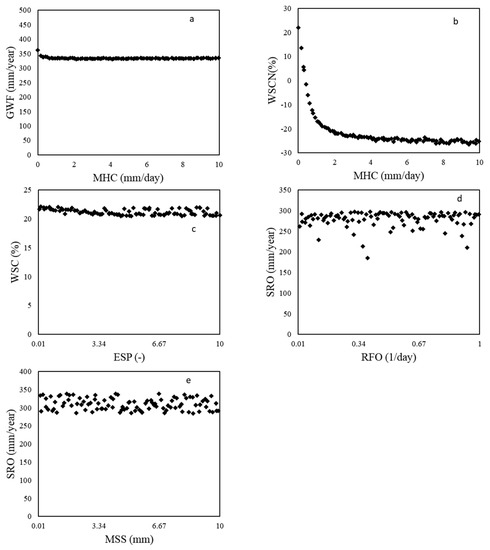
Figure A1.
The relationships between ground water flow (GWF), water content change (WSC) and surface runoff (SRO) with changes in parameters with NRMSE > 1% (minimum hydraulic conductivity (MHC), ammonium immobilised fraction (AIF), specific fertiliser dissolution rate (SFD) and maximum autotrophic nitrification rate (MAN)).
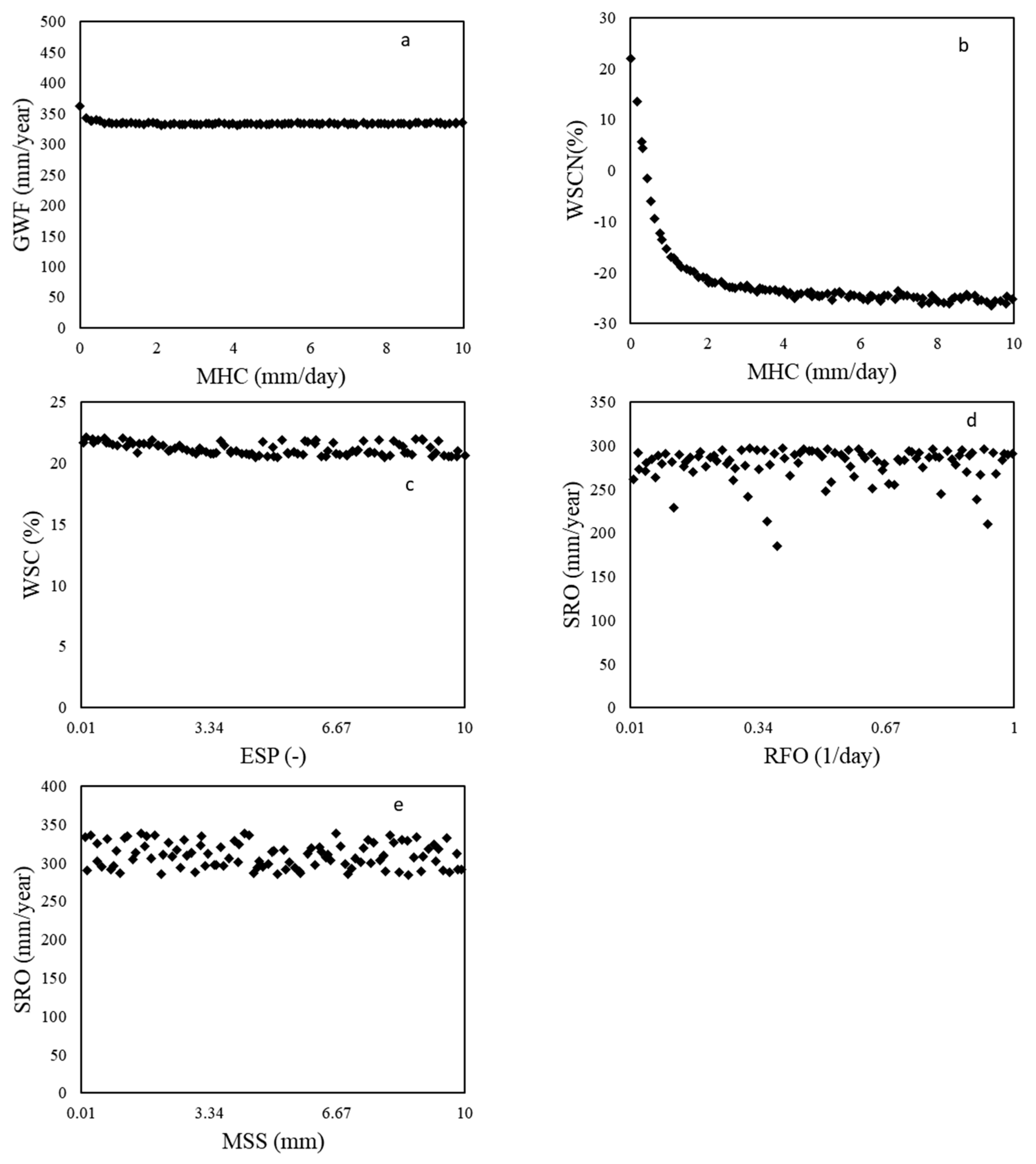
Figure A2.
Response of grains (GDM), leaves (LDM) and stems (SDM) dry matter to the parameters—distance between drainpipes (DBD), minimum roughness length (MRL), drain pipe level (DPL) and ammonium immobilised fraction (AIF). All with NRMSD > 1% over the simulation period.
Figure A2.
Response of grains (GDM), leaves (LDM) and stems (SDM) dry matter to the parameters—distance between drainpipes (DBD), minimum roughness length (MRL), drain pipe level (DPL) and ammonium immobilised fraction (AIF). All with NRMSD > 1% over the simulation period.
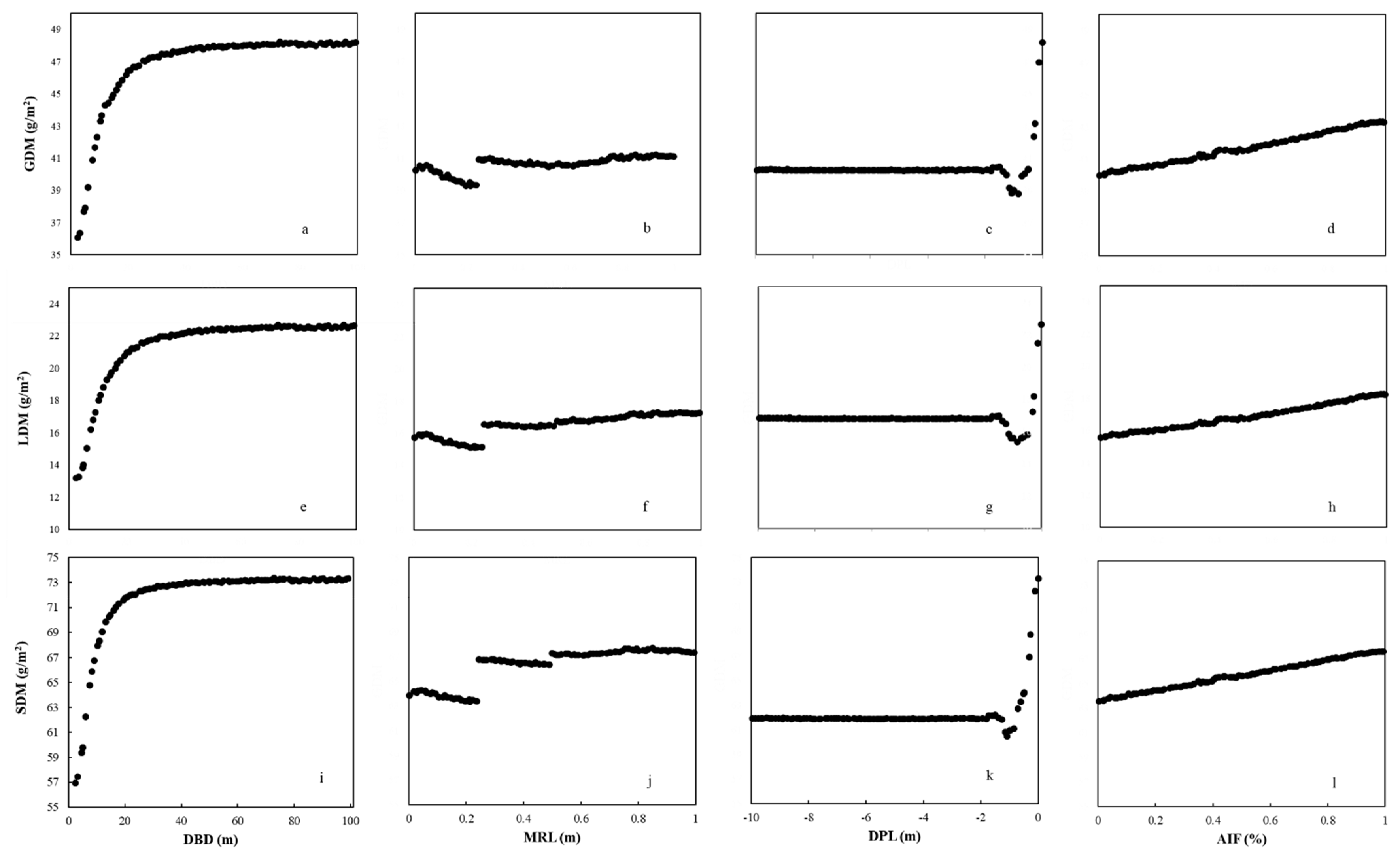
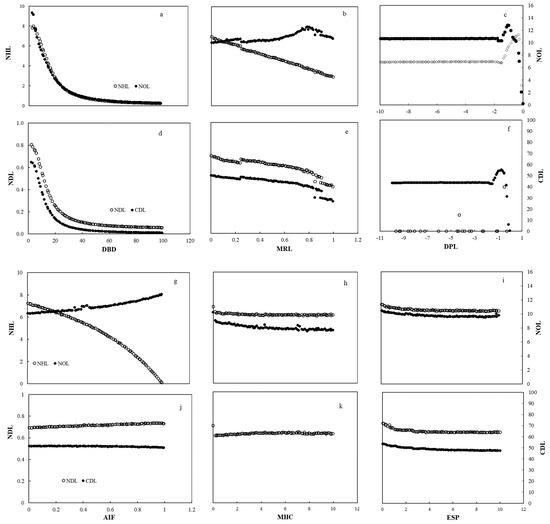
Figure A3.
Relationships between simulated leached losses of N and C to their most influential parameters (by NRMSD). Simulated variables: NHL: NH4 leach; NOL: NO3 leach; NDL: N dissolve leach; CDL: C dissolve leach. Model parameters: DBD: distance between drainpipes; MRL: minimum roughness length; DPL: drain pipe level; AIF: ammonium immobilised fraction; MHC: minimum hydraulic conductivity; and ESP: empirical scale in pore shape.
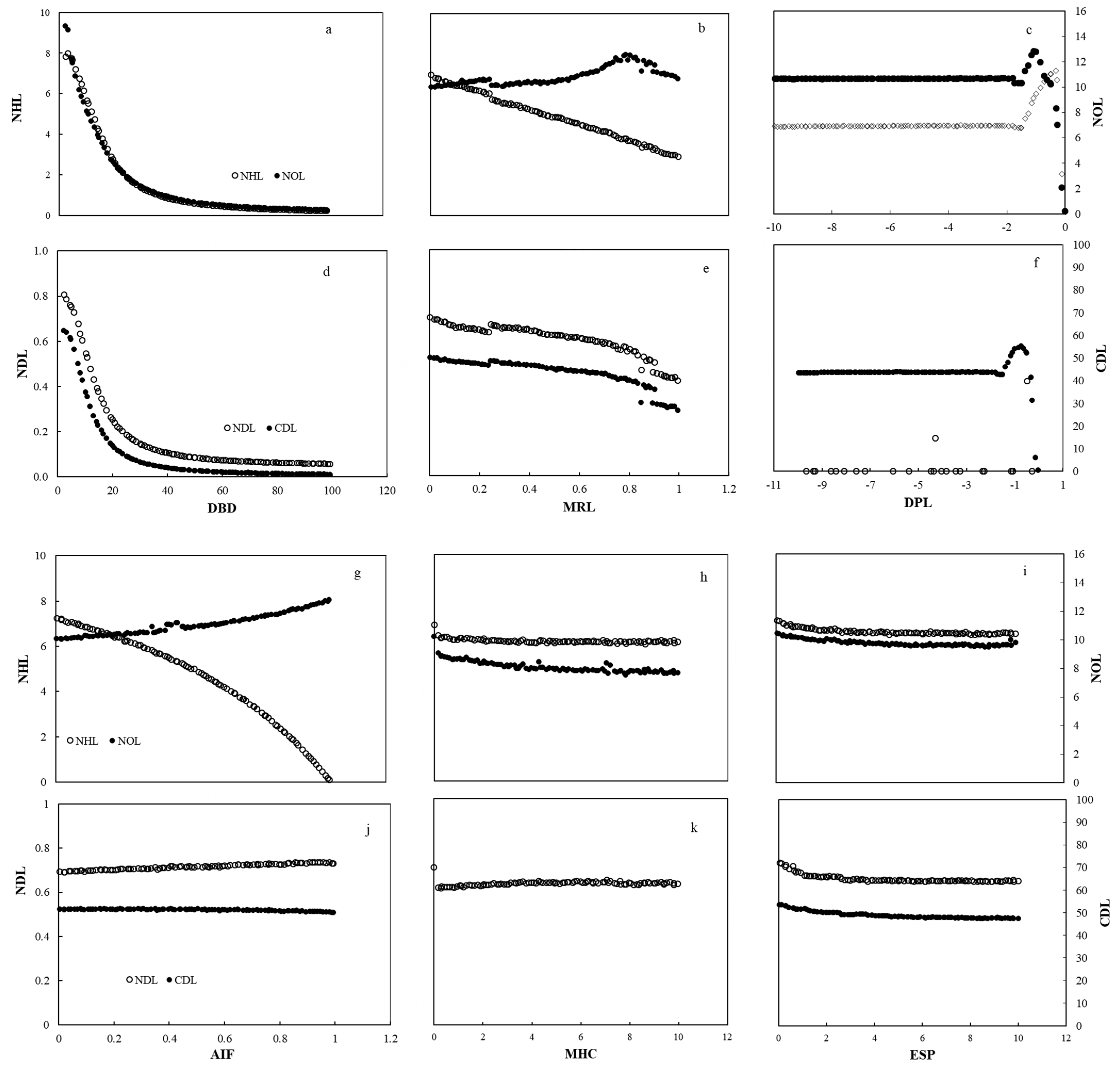
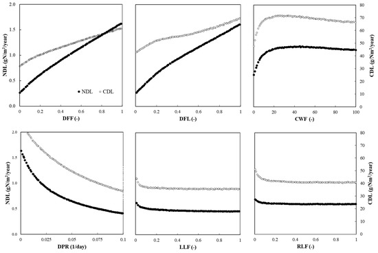
Figure A4.
The relationships between leached losses of N and C and the parameters with NRMSEs higher than 1% (CDL: C dissolve leach; NDL: N dissolve leach; DFF: dissolved fraction from fresh litter; DFL: dissolved fraction in litter; CWF: coefficient in water function in the process of organic matter decomposition; DPR: potential decomposition rate of dissolved organic matter; LLF: litter unit loss fraction; RLF: residue unit loss fraction).
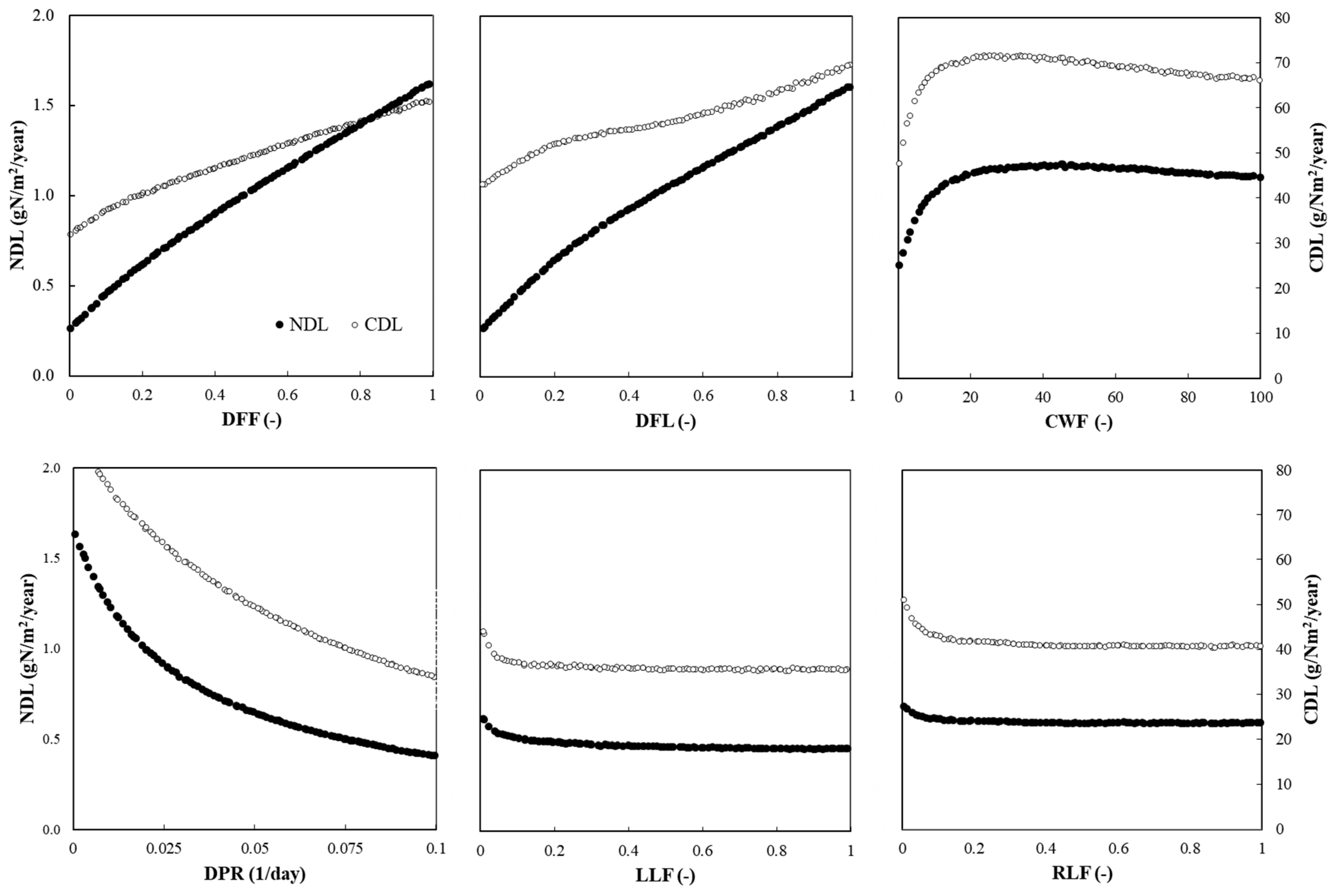
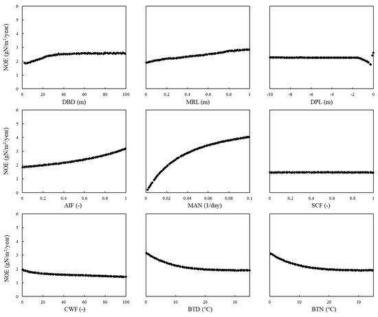
Figure A5.
The relationships between NOE and sensitive parameters (DBD: distance between drainpipes; MRL: minimum roughness length; DPL: drain pipe level; AIF: ammonium immobilised fraction; MAN: maximum autotrophic nitrification rate; SCF: soil cover fraction prevent infiltration; CWF: coefficient in water function in the process of organic matter decomposition; BTD: base temp to unity denitrification; BTN: base temp to unity nitrification).
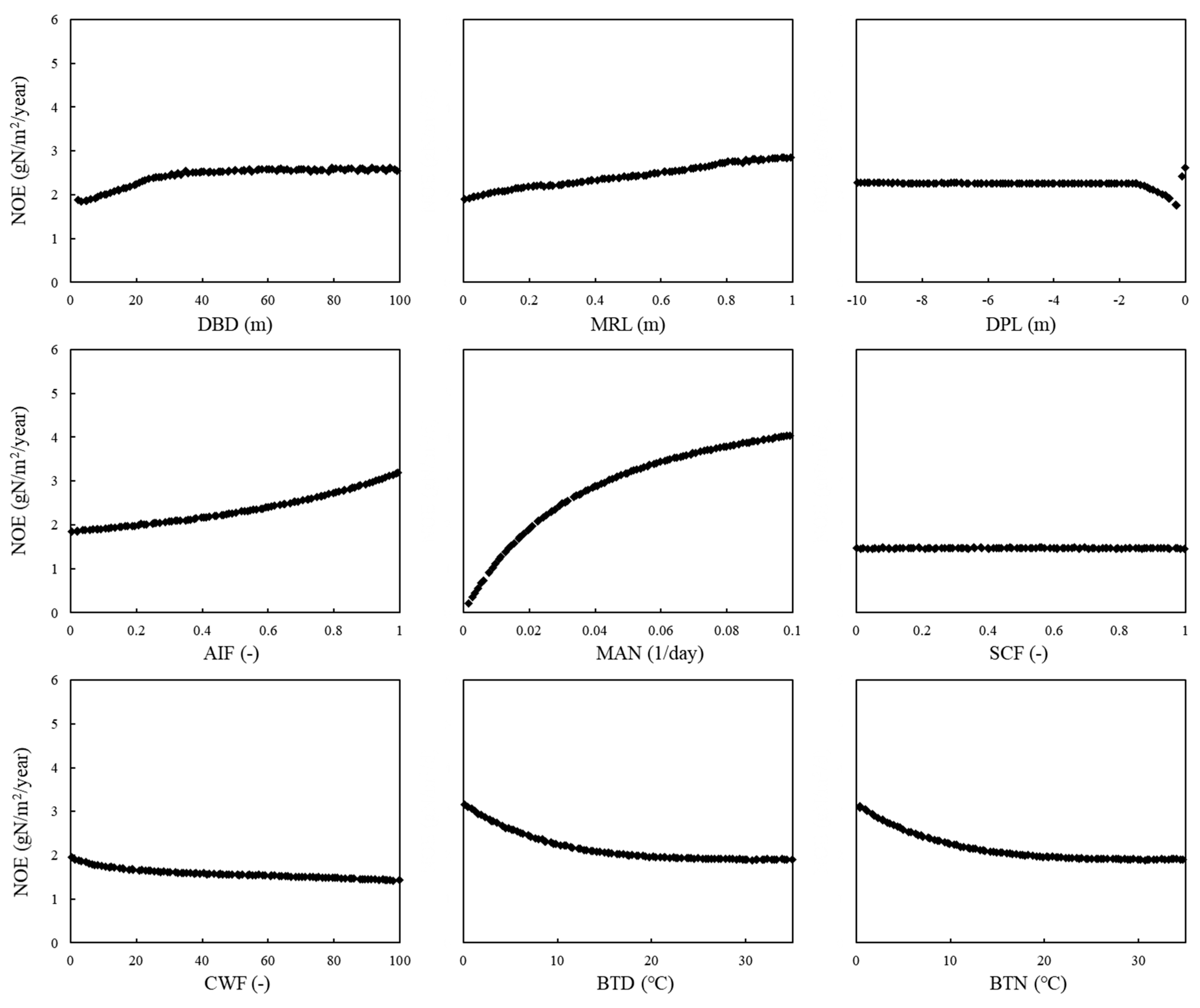
Figure A6.
The relationships between carbon dissolved release (DRE) and sensitive parameters (DBD: distance between drainpipes; MRL: minimum roughness length; DPL: drain pipe level; MHC: minimum hydraulic conductivity; HPD: humus potential decomposition rate; LLF: litter unit loss fraction; OAW: optimal available water content; HFD: humus fraction from fresh litter; DFF: dissolved fraction from fresh litter; DFL: dissolved fraction in litter; RLT: residue to litter transfer fraction; FLD: fresh litter potential decomposition rate; RLF: residue unit loss fraction; DPR: dissolved potential decomposition rate; BTM: base temp to unity mineralization).
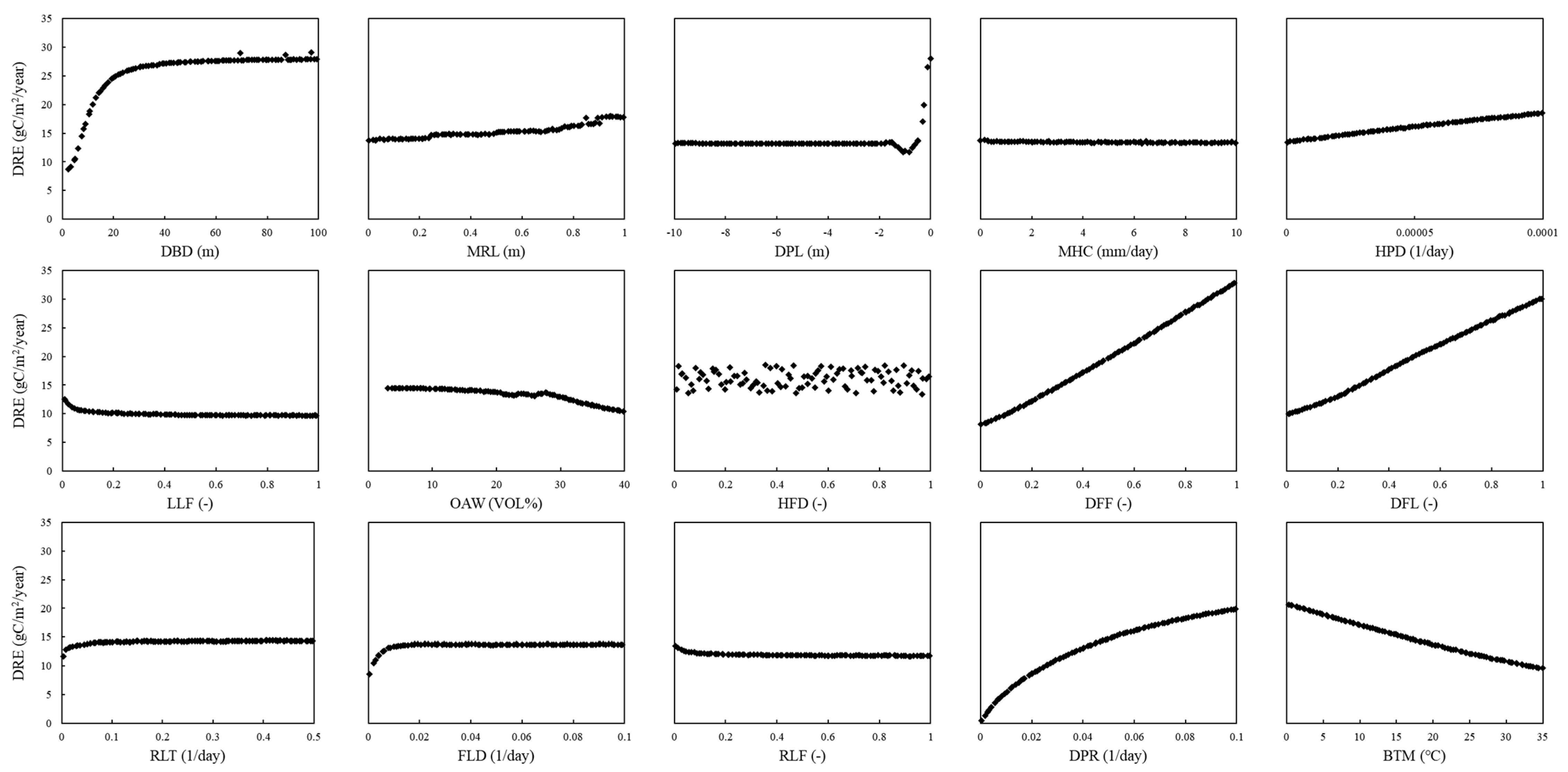
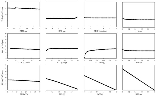
Figure A7.
The relationships between fresh litter release (FLR) and sensitive parameters (MRL: minimum roughness length; DPL: drain pipe level; MHC: minimum hydraulic conductivity; LLF: litter unit loss fraction; OAW: optimal available water content; RLT: residue to litter transfer fraction; FLD: potential decomposition rate of fresh litter; RLF: residue unit loss fraction; BTM: base temp to unity mineralization; DFL: dissolved fraction in litter; DFF: dissolved fraction from fresh litter; HFL: partitioning fraction to humus from decomposed fresh litter).
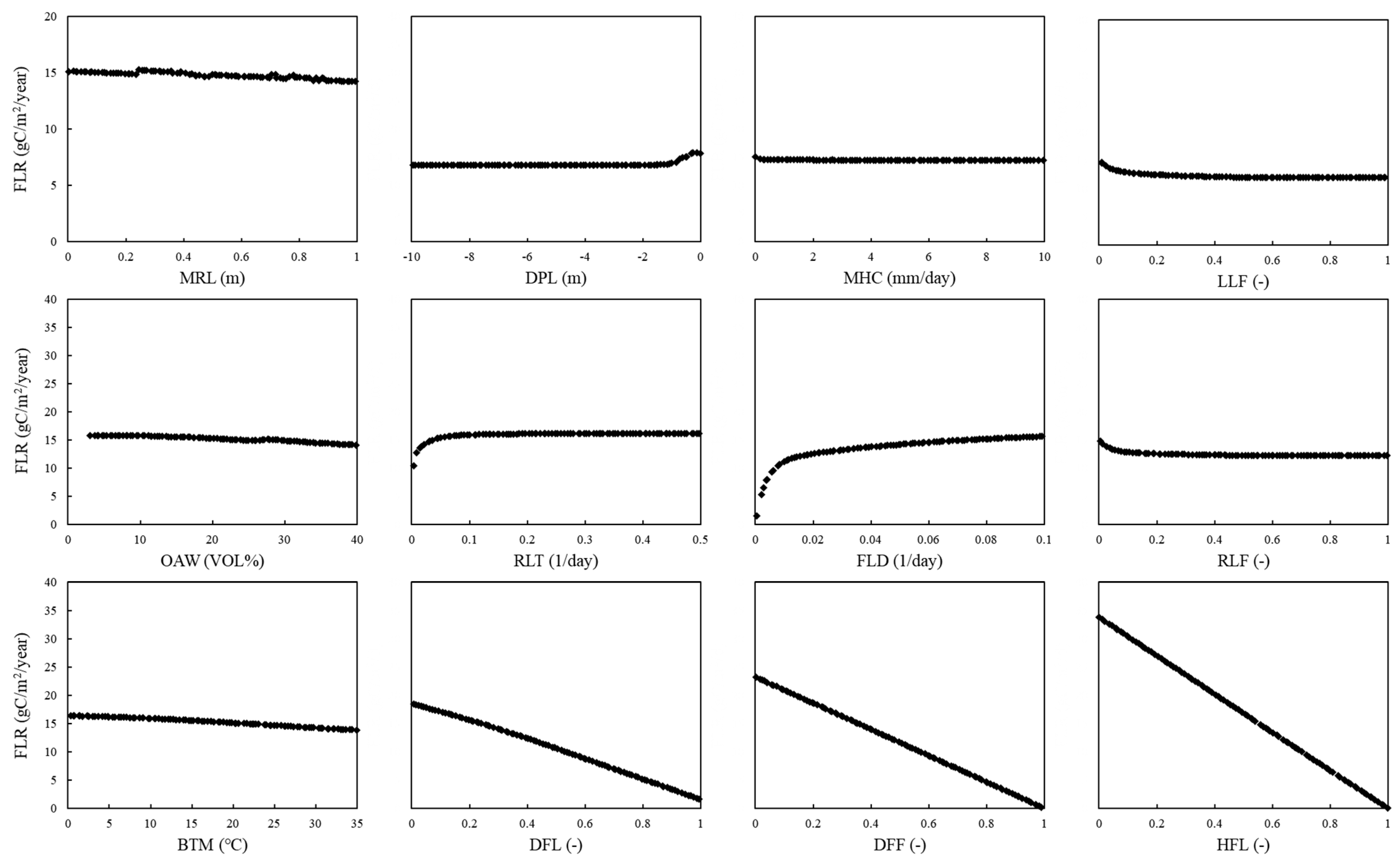
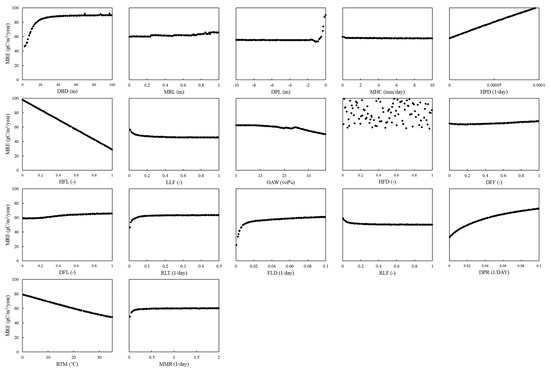
Figure A8.
The relationships between microbial release (MRE) and sensitive parameters (DBD: distance between drainpipes; MRL: minimum roughness length; DPL: drain pipe level; MHC: minimum hydraulic conductivity; HPD: humus potential decomposition rate; HFL: partitioning fraction to humus from decomposed fresh litter; LLF: litter unit loss fraction; OAW: optimal available water content; HFD: partitioning fraction to humus from decomposed dissolved organic matter; DFF: dissolved fraction from fresh litter; DFL: dissolved fraction in litter; RLT: residue to litter transfer fraction; FLD: potential decomposition rate of fresh litter; RLF: Residue unit loss fraction; DPR: potential decomposition rate of dissolved organic matter; BTM: base temp to unity mineralization; MMR: microbial maintenance respiration rate).

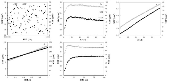
Figure A9.
Relationships between changes in soil organic C and N pools and the parameters they are most sensitive to over the simulation period. NHP: N humus pool; CHP: C humus pool; NDP: N dissolve pool; CDP: C dissolve pool; HPD: humus potential decomposition rate; CWF: coefficient in water function; DFL: dissolved fraction in litter; HFL: humus fraction from fresh litter; DBD: distance between drainpipes.
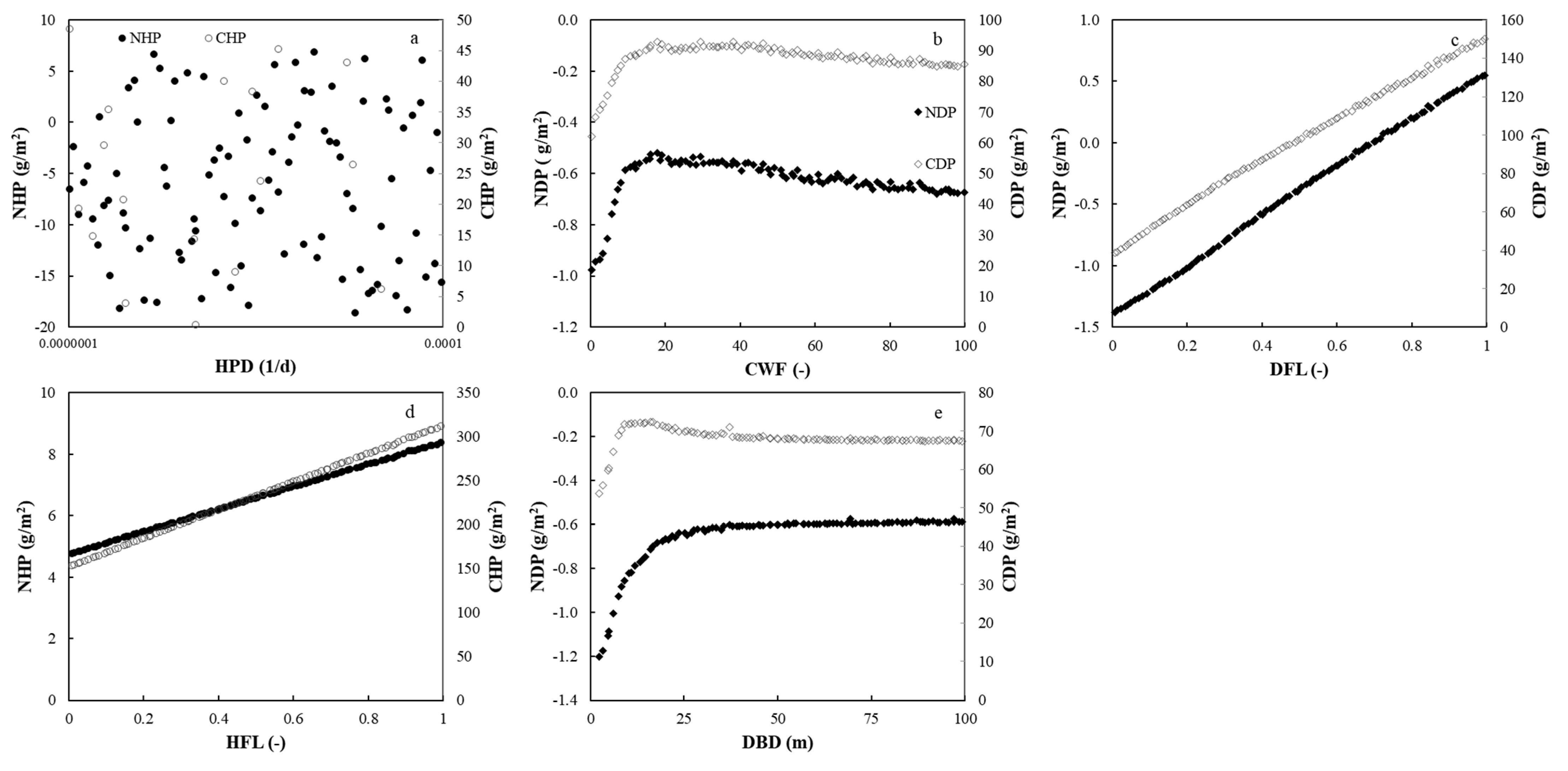
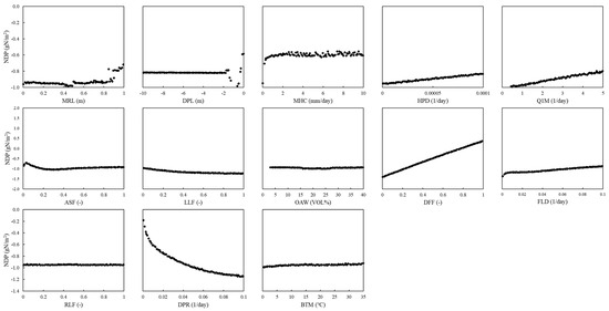
Figure A10.
The relationships between nitrogen dissolved pool (NDP) and sensitive parameters (MRL: minimum roughness length; DPL: drain pipe level; MHC: minimum hydraulic conductivity; HPD: humus potential decomposition rate; Q1M: Q10 value for mineralization; ASF: assimilation factor; LLF: litter unit loss fraction; OAW: optimal available water content; DFF: dissolved fraction from fresh litter; FLD: potential decomposition rate of fresh litter; RLF: residue unit loss fraction; DPR: potential decomposition rate of dissolved organic matter; BTM: base temp to unity mineralization).
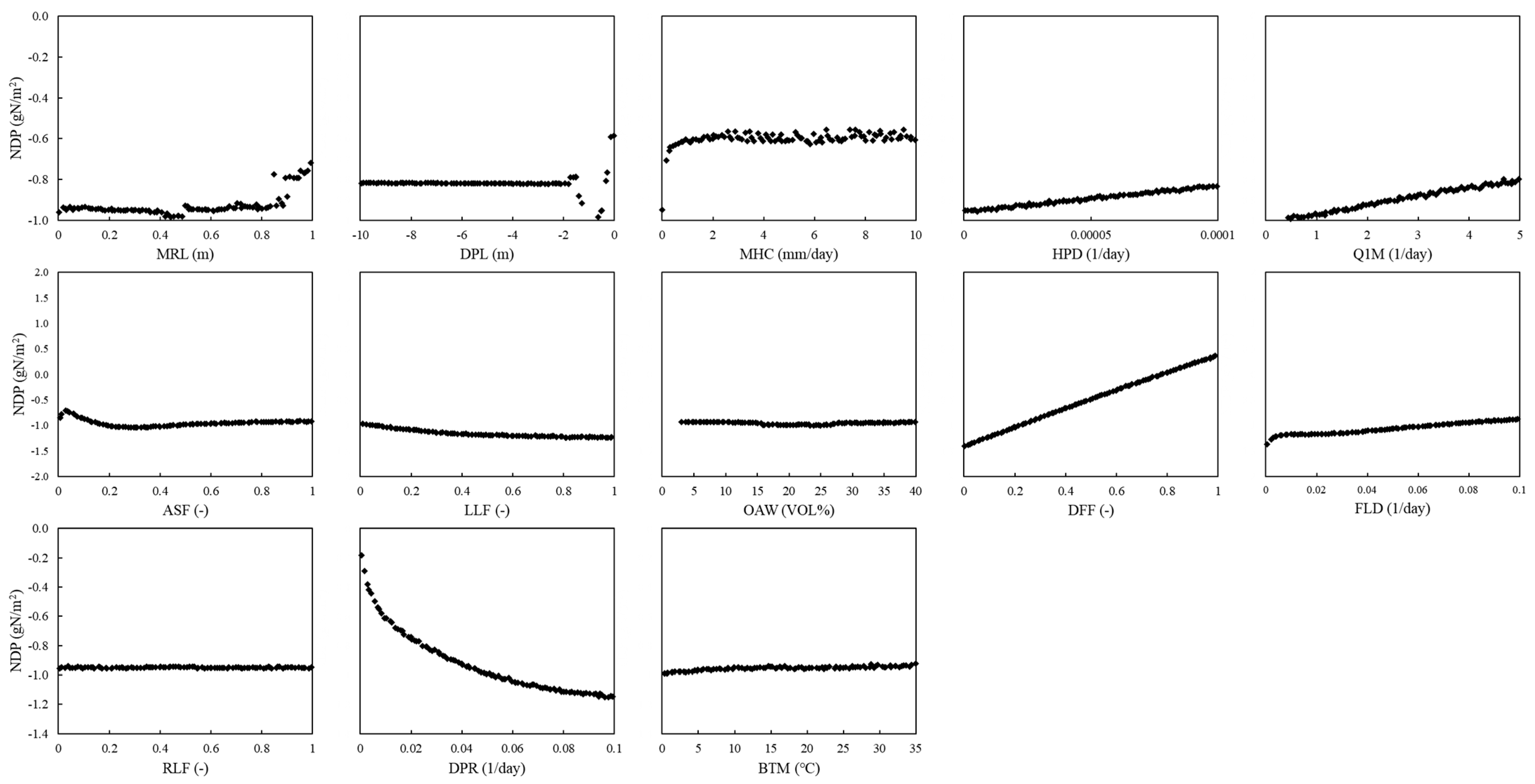
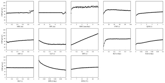
Figure A11.
The relationships between carbon dissolved pool (CDP) simulations and sensitive parameters (MRL: minimum roughness length; DPL: drain pipe level; MHC: minimum hydraulic conductivity; CWF: coefficient in water function in the process of organic matter decomposition; Q1M: Q10 value for mineralization; ASF: assimilation factor; LLF: litter unit loss fraction; DFF: dissolved fraction from fresh litter; RLT: residue to litter transfer fraction; FLD: potential decomposition rate of fresh litter; RLF: residue unit loss fraction; DPR: potential decomposition rate of dissolved organic matter; BTM: base temp to unity mineralization).
References
- Krishnan, P.; Aggarwal, P. Global sensitivity and uncertainty analyses of a web based crop simulation model (web InfoCrop wheat) for soil parameters. Plant. Soil 2018, 423, 443–463. [Google Scholar] [CrossRef]
- Leolini, L.; Bregaglio, S.; Moriondo, M.; Ramos, M.C.; Bindi, M.; Ginaldi, F. A model library to simulate grapevine growth and development: Software implementation, sensitivity analysis and field level application. Eur. J. Agron. 2018, 99, 92–105. [Google Scholar] [CrossRef]
- Eitzinger, J.; Thaler, S.; Schmid, E.; Strauss, F.; Ferrise, R.; Moriondo, M.; Bindi, M.; Palosuo, T.; Rötter, R.; Kersebaum, K.C.; et al. Sensitivities of crop models to extreme weather conditions during flowering period demonstrated for maize and winter wheat in Austria. J. Agric. Sci. 2012, 151, 813–835. [Google Scholar] [CrossRef]
- Sommer, R.; Mukalama, J.; Kihara, J.; Koala, S.; Winowiecki, L.; Bossio, D. Nitrogen dynamics and nitrous oxide emissions in a long-term trial on integrated soil fertility management in Western Kenya. Nutr. Cycl. Agroecosyst. 2016, 105, 229–248. [Google Scholar] [CrossRef]
- Liu, X.Y.; Zhao, Y.C.; Shi, X.Z.; Liu, Y.; Wang, S.H.; Yu, D.S. Sensitivity and uncertainty analysis of CENTURY-modeled SOC dynamics in upland soils under different climate-soil-management conditions: A case study in China. J. Soils Sediments 2017, 17, 85–96. [Google Scholar] [CrossRef]
- Wu, R.; Lawes, R.; Oliver, Y.; Fletcher, A.; Chen, C. How well do we need to estimate plant-available water capacity to simulate water-limited yield potential? Agric. Water Manag. 2019, 212, 441–447. [Google Scholar] [CrossRef]
- Grassini, P.; van Bussel, L.G.J.; van Wart, J.; Wolf, J.; Claessens, L.; Yang, H.; Boogaard, H.; de Groot, H.; van Ittersum, M.K.; Cassman, K.G. How good is good enough? Data requirements for reliable crop yield simulations and yield-gap analysis. Field Crop. Res. 2015, 177, 49–63. [Google Scholar] [CrossRef] [Green Version]
- He, J.; Dukes, M.D.; Hochmuth, G.J.; Jones, J.W.; Graham, W.D. Evaluation of sweet corn yield and nitrogen leaching with CERES-Maize considering input parameter uncertainties. Trans. ASABE 2011, 54, 1257–1268. [Google Scholar] [CrossRef]
- Marino, S.; Hogue, I.B.; Ray, C.J.; Kirschner, D.E. A methodology for performing global uncertainty and sensitivity analysis in systems biology. J. Theor. Biol. 2008, 254, 178–196. [Google Scholar] [CrossRef] [Green Version]
- Specka, X.; Nendel, C.; Wieland, R. Analysing the parameter sensitivity of the agro-ecosystem model MONICA for different crops. Eur. J. Agron. 2015, 71, 73–87. [Google Scholar] [CrossRef]
- Jabloun, M.; Li, X.X.; Zhang, X.Y.; Tao, F.L.; Hu, C.S.; Olesen, J.E. Sensitivity of simulated crop yield and nitrate leaching of the wheat-maize cropping system in the North China Plain to model parameters. Agric. For. Meteorol. 2018, 263, 25–40. [Google Scholar] [CrossRef] [Green Version]
- Sarrazin, F.; Pianosi, F.; Wagener, T. Global sensitivity analysis of environmental models: Convergence and validation. Environ. Model. Softw. 2016, 79, 135–152. [Google Scholar] [CrossRef] [Green Version]
- Wu, L.; McGechan, M.B.; McRoberts, N.; Baddeley, J.A.; Watson, C.A. SPACSYS: Integration of a 3D root architecture component to carbon, nitrogen and water cycling-model description. Ecol. Model. 2007, 200, 343–359. [Google Scholar] [CrossRef]
- Abalos, D.; Cardenas, L.M.; Wu, L.H. Climate change and N2O emissions from South West England grasslands: A modelling approach. Atmos. Environ. 2016, 132, 249–257. [Google Scholar] [CrossRef]
- Liang, S.; Li, Y.F.; Zhang, X.B.; Sun, Z.G.; Sun, N.; Duan, Y.H.; Xu, M.G.; Wu, L.H. Response of crop yield and nitrogen use efficiency for wheat-maize cropping system to future climate change in northern China. Agric. For. Meteorol. 2018, 262, 310–321. [Google Scholar] [CrossRef]
- Zhang, X.B.; Xu, M.G.; Sun, N.; Xiong, W.; Huang, S.M.; Wu, L.H. Modelling and predicting crop yield, soil carbon and nitrogen stocks under climate change scenarios with fertiliser management in the North China Plain. Geoderma 2016, 265, 176–186. [Google Scholar] [CrossRef]
- Zhang, X.B.; Sun, Z.G.; Liu, J.; Ouyang, Z.; Wu, L.H. Simulating greenhouse gas emissions and stocks of carbon and. nitrogen in soil from a long-term no-till system in the North China Plain. Soil Tillage Res. 2018, 178, 32–40. [Google Scholar] [CrossRef]
- Perego, A.; Wu, L.; Gerosa, G.; Finco, A.; Chiazzese, M.; Amaducci, S. Field evaluation combined with modelling analysis to study fertilizer and tillage as factors affecting N2O emissions: A case study in the Po valley (Northern Italy). Agric. Ecosyst. Environ. 2016, 225, 72–85. [Google Scholar] [CrossRef]
- Wu, L.; Zhang, X.; Griffith, B.A.; Misselbrook, T.H. Sustainable grassland systems: A modelling perspective based on the North Wyke Farm Platform. Eur. J. Soil Sci. 2016, 67, 397–408. [Google Scholar] [CrossRef] [Green Version]
- He, W.; Yang, J.Y.; Zhou, W.; Drury, C.F.; Yang, X.M.; Reynolds, W.D.; Wang, H.; He, P.; Li, Z.T. Sensitivity analysis of crop yields, soil water contents and nitrogen leaching to precipitation, management practices and soil hydraulic properties in semi-arid and humid regions of Canada using the DSSAT model. Nutr. Cycl. Agroecosystems 2016, 106, 201–215. [Google Scholar] [CrossRef]
- Zhao, G.; Bryan, B.A.; Song, X.D. Sensitivity and uncertainty analysis of the APSIM-wheat model: Interactions between cultivar, environmental, and management parameters. Ecol. Model. 2014, 279, 1–11. [Google Scholar] [CrossRef]
- Yan, W.-J.; Wan, H.-P.; Ren, W.-X. Analytical local and global sensitivity of power spectrum density functions for structures subject to stochastic excitation. Comput. Struct. 2017, 182, 325–336. [Google Scholar] [CrossRef]
- Ginot, V.; Gaba, S.; Beaudouin, R.; Aries, F.; Monod, H. Combined use of local and ANOVA-based global sensitivity analyses for the investigation of a stochastic dynamic model: Application to the case study of an individual-based model of a fish population. Ecol. Model. 2006, 193, 479–491. [Google Scholar] [CrossRef]
- Loosvelt, L.; Vernieuwe, H.; Pauwels, V.R.N.; de Baets, B.; Verhoest, N.E.C. Local sensitivity analysis for compositional data with application to soil texture in hydrologic modelling. Hydrol. Earth Syst. Sci. 2013, 17, 461–478. [Google Scholar] [CrossRef] [Green Version]
- Krishna, N.A.; Pennington, H.M.; Coppola, C.D.; Eisenberg, M.C.; Schugart, R.C. Connecting local and global sensitivities in a mathematical model for wound healing. Bull. Math. Biol. 2015, 77, 2294–2324. [Google Scholar] [CrossRef]
- Nguyen-Tuan, L.; Lahmer, T.; Datcheva, M.; Schanz, T. Global and local sensitivity analyses for coupled thermo–hydro–mechanical problems. Int. J. Numer. Anal. Methods Geomech. 2017, 41, 707–720. [Google Scholar] [CrossRef]
- Link, K.G.; Stobb, M.T.; Di Paola, J.; Neeves, K.B.; Fogelson, A.L.; Sindi, S.S.; Leiderman, K. A local and global sensitivity analysis of a mathematical model of coagulation and platelet deposition under flow. PLoS ONE 2018, 13, e0200917. [Google Scholar] [CrossRef] [PubMed]
- Naves, J.; Rieckermann, J.; Cea, L.; Puertas, J.; Anta, J. Global and local sensitivity analysis to improve the understanding of physically-based urban wash-off models from high-resolution laboratory experiments. Sci. Total Environ. 2020, 709, 136152. [Google Scholar] [CrossRef] [PubMed]
- Li, Y.; Liu, Y.; Harris, P.; Sint, H.; Murray, P.J.; Lee, M.; Wu, L. Assessment of soil water, carbon and nitrogen cycling in reseeded grassland on the North Wyke Farm Platform using a process-based model. Sci. Total Environ. 2017, 603-604, 27–37. [Google Scholar] [CrossRef] [PubMed] [Green Version]
- Liu, Y.; Li, Y.; Harris, P.; Cardenas, L.; Dunn, R.M.; Sint, H.; Murray, P.; Lee, M.; Wu, L. Modelling field scale spatial variation in water run-off, soil moisture, N2O emissions and herbage biomass of a grazed pasture using the SPACSYS model. Geoderma 2018, 315, 49–58. [Google Scholar] [CrossRef]
- Wu, L.; Rees, R.M.; Tarsitano, D.; Zhang, X.B.; Jones, S.K.; Whitmore, A.P. Simulation of nitrous oxide emissions at field scale using the SPACSYS model. Sci. Total Environ. 2015, 530, 76–86. [Google Scholar] [CrossRef] [Green Version]
- Wu, L.; Shepherd, A. Special features of the SPACSYS modeling package and procedures for parameterization and validation. In Methods of Introducing System Models into Agricultural Research; Ahuja, L.R., Ma, L., Eds.; ASA, CSSA & SSSA: Madison, WI, USA, 2011; pp. 117–154. [Google Scholar]
- Saltelli, A.; Aleksankina, K.; Becker, W.; Fennell, P.; Ferretti, F.; Holst, N.; Li, S.; Wu, Q. Why so many published sensitivity analyses are false: A systematic review of sensitivity analysis practices. Environ. Model. Softw. 2019, 114, 29–39. [Google Scholar] [CrossRef]
- Ballantine, D.J.; Tanner, C.C. Controlled drainage systems to reduce contaminant losses and optimize productivity from New Zealand pastoral systems. N. Z. J. Agric. Res. 2013, 56, 171–185. [Google Scholar] [CrossRef]
- Ritzema, H.P. Drain for gain: Managing salinity in irrigated lands—A review. Agric. Water Manag. 2016, 176, 18–28. [Google Scholar] [CrossRef] [Green Version]
- Jouni, H.J.; Liaghat, A.; Hassanoghli, A.; Henk, R. Managing controlled drainage in irrigated farmers’ fields: A case study in the Moghan plain, Iran. Agric. Water Manag. 2018, 208, 393–405. [Google Scholar] [CrossRef]
- Tomic, F.; Kricka, T.; Simunic, I.; Petosic, D.; Voca, N.; Jukic, Z. Effect of drainage systems on the water release rate in the process of drying wheat and corn grain. Irrig. Drain. 2007, 56, 107–113. [Google Scholar] [CrossRef]
- Helmers, M.; Christianson, R.; Brenneman, G.; Lockett, D.; Pederson, C. Water table, drainage, and yield response to drainage water management in southeast Iowa. J. Soil Water Conserv. 2012, 67, 495–501. [Google Scholar] [CrossRef]
- Carstensen, M.V.; Poulsen, J.R.; Ovesen, N.B.; Børgesen, C.D.; Hvid, S.K.; Kronvang, B. Can controlled drainage control agricultural nutrient emissions? Evidence from a BACI experiment combined with a dual isotope approach. Hydrol. Earth Syst. Sci. Discuss. 2016, 1–17. [Google Scholar] [CrossRef]
- Borin, M.; Bonaiti, G.; Giardini, L. Controlled drainage and wetlands to reduce agricultural pollution: A lysimetric study. J. Environ. Qual. 2001, 30, 1330–1340. [Google Scholar] [CrossRef] [PubMed]
- Mohammadzadeh-Habili, J.; Mostafazadeh-Fard, B. Hydraulic calculation of field drain pipe diameter: Using the theory of spatially-varied flow with increasing discharge. Biosyst. Eng. 2010, 106, 559–563. [Google Scholar] [CrossRef]
- Ma, J.M.; Daggupaty, S.M. Stability dependence of height scales and effective roughness lengths of momentum and heat transfer over roughness changes. Bound. Layer Meteorol. 1998, 88, 145–160. [Google Scholar] [CrossRef]
- Martinez-Agirre, A.; Alvarez-Mozos, J.; Lievens, H.; Verhoest, N.E.C. Influence of surface roughness measurement scale on radar backscattering in different agricultural soils. IEEE Trans. Geosci. Remote Sens. 2017, 55, 5925–5936. [Google Scholar] [CrossRef] [Green Version]
- Wang, S.G.; Li, X.; Han, X.J.; Jin, R. Estimation of surface soil moisture and roughness from multi-angular ASAR imagery in the Watershed Allied Telemetry Experimental Research (WATER). Hydrol. Earth Syst. Sci. 2011, 15, 1415–1426. [Google Scholar] [CrossRef] [Green Version]
- Moret-Fernández, D.; Latorre, B.; Giner, M.L.; Ramos, J.; Alados, C.L.; Castellano, C.; López, M.V.; Jimenez, J.J.; Pueyo, Y. Estimation of the soil hydraulic properties from the transient infiltration curve measured on soils affected by water repellency. CATENA 2019, 178, 298–306. [Google Scholar] [CrossRef]
- Fernandez-Galvez, J.; Pollacco, J.A.P.; Lassabatere, L.; Angulo-Jaramillo, R.; Carrick, S. A general Beerkan estimation of soil transfer parameters method predicting hydraulic parameters of any unimodal water retention and hydraulic conductivity curves: Application to the kosugi soil hydraulic model without using particle size distribution data. Adv. Water Resour. 2019, 129, 118–130. [Google Scholar] [CrossRef]
- Pinheiro, E.A.R.; van Lier, Q.D.; Simunek, J. The role of soil hydraulic properties in crop water use efficiency: A process-based analysis for some Brazilian scenarios. Agric. Syst. 2019, 173, 364–377. [Google Scholar] [CrossRef] [Green Version]
- Vereecken, H.; Kamai, T.; Harter, T.; Kasteel, R.; Hopmans, J.; Vanderborght, J. Explaining soil moisture variability as a function of mean soil moisture: A stochastic unsaturated flow perspective. Geophys. Res. Lett. 2007, 34, 6. [Google Scholar] [CrossRef] [Green Version]
- Kang, S.Z.; Zhang, L.; Liang, Y.L.; Hu, X.T.; Cai, H.J.; Gu, B.J. Effects of limited irrigation on yield and water use efficiency of winter wheat in the Loess Plateau of China. Agric. Water Manag. 2002, 55, 203–216. [Google Scholar] [CrossRef]
- Lawless, C.; Semenov, M.A.; Jamieson, P.D. Quantifying the effect of uncertainty in soil moisture characteristics on plant growth using a crop simulation model. Field Crop. Res. 2008, 106, 138–147. [Google Scholar] [CrossRef]
- Gao, Y.J.; Li, Y.; Zhang, J.C.; Liu, W.G.; Dang, Z.P.; Cao, W.X.; Qiang, Q. Effects of mulch, N fertilizer, and plant density on wheat yield, wheat nitrogen uptake, and residual soil nitrate in a dryland area of China. Nutr. Cycl. Agroecosyst. 2009, 85, 109–121. [Google Scholar] [CrossRef]
- Raun, W.R.; Johnson, G.V. Improving nitrogen use efficiency for cereal production. Agron. J. 1999, 91, 357–363. [Google Scholar] [CrossRef] [Green Version]
- Zorb, C.; Ludewig, U.; Hawkesford, M.J. Perspective on wheat yield and quality with reduced nitrogen supply. Trends Plant Sci. 2018, 23, 1029–1037. [Google Scholar] [CrossRef] [PubMed] [Green Version]
- Wang, X.; He, X.; Williams, J.R.; Izaurralde, R.C.; Atwood, J.D. Sensitivity and uncertainty analyses of crop yields and soil organic carbon simulated with EPIC. Trans. ASAE 2005, 48, 1041–1054. [Google Scholar] [CrossRef]
- Ibrahim, M.; Cao, C.G.; Zhan, M.; Li, C.F.; Iqbal, J. Changes of CO2 emission and labile organic carbon as influenced by rice straw and different water regimes. Int. J. Environ. Sci. Technol. 2015, 12, 263–274. [Google Scholar] [CrossRef]
- Jugsujinda, A.; Delaune, R.D.; Lindau, C.W.; Sulaeman, E.; Pezeshki, S.R. Factors controlling carbon dioxide and methane production in acid sulfate soils. Water Air Soil Pollut. 1996, 87, 345–355. [Google Scholar] [CrossRef]
- Pires, C.V.; Schaefer, C.; Hashigushi, A.K.; Thomazini, A.; Filho, E.I.F.; Mendonca, E.S. Soil organic carbon and nitrogen pools drive soil C-CO2 emissions from selected soils in Maritime Antarctica. Sci. Total Environ. 2017, 596, 124–135. [Google Scholar] [CrossRef] [PubMed]
- Liu, Y.; Hu, C.; Mohamed, I.; Wang, J.; Zhang, G.S.; Li, Z.G.; Chen, F. Soil CO2 emissions and drivers in rice-wheat rotation fields subjected to different long-term fertilization practices. Clean Soil Air Water 2016, 44, 867–876. [Google Scholar] [CrossRef]
- Oorts, K.; Merckx, R.; Gréhan, E.; Labreuche, J.; Nicolardot, B. Determinants of annual fluxes of CO2 and N2O in long-term no-tillage and conventional tillage systems in northern France. Soil Tillage Res. 2007, 95, 133–148. [Google Scholar] [CrossRef]
- Rodrigo, A.; Recous, S.; Neel, C.; Mary, B. Modelling temperature and moisture effects on C-N transformations in soils: Comparison of nine models. Ecol. Model. 1997, 102, 325–339. [Google Scholar] [CrossRef]
Publisher’s Note: MDPI stays neutral with regard to jurisdictional claims in published maps and institutional affiliations. |
© 2021 by the authors. Licensee MDPI, Basel, Switzerland. This article is an open access article distributed under the terms and conditions of the Creative Commons Attribution (CC BY) license (https://creativecommons.org/licenses/by/4.0/).

