Abstract
Adjusting tillage parameters according to soil conditions can reduce energy consumption. In this study, the working parameters and soil physical parameters of plowing were determined using a designed electric suspension platform and soil instrument. The soil conditions were classified into three physical states, namely ‘hard’, ‘zero’, and ‘soft’ using a fuzzy C-means clustering algorithm, taking the soil moisture content and cone penetration resistance as the grading indexes. The Takagi–Sugeno (T–S) fuzzy neural network classifier was constructed using traction resistance, operating velocity, and plowing depth as inputs to indirectly identify the soil’s physical state. The results show that when 280 groups of test data were used to verify the model, 264 groups were correctly identified, indicating a soil physical state identification accuracy of 94.29%. The T–S fuzzy neural network prediction model can achieve the real-time and accurate physical state identification of paddy soil during plowing.
1. Introduction
Energy used for soil farming accounts for 50% of the total agricultural energy consumption in China [1]. Some scholars [2,3] have achieved good results by optimizing the geometric parameters of the plowshare to reduce friction between the plowshare and soil, and hence reduce energy consumption during plowing. For the soil–tool contact system, reducing the energy consumption only by optimizing the geometric parameters of the plowshare is not enough. Relevant studies [4,5] have shown that the factors affecting plowing energy consumption include the plowshare geometric parameters, soil parameters, and working parameters (forward speed and plowing depth). Therefore, the effect of soil conditions on energy consumption should also be considered in the process of plowing.
Soil conditions have an important effect on energy consumption. Adjusting the working parameters according to the soil’s physical state during plowing, that is, integrating agricultural machinery and agronomy, can reduce the impact of the spatial variation of the soil’s physical properties on energy consumption [6]. The studies in [7,8] also emphasized the importance of soil parameters on energy consumption during plowing by establishing a mathematical model that correlates energy consumption with soil parameters. When plowing is carried out, the spatial difference in the physical properties of the soil causes a change in the traction resistance and unnecessary energy consumption [9], reducing the power and cost-effectiveness of tractors. Therefore, the soil state should be considered during operation, which is necessary for adjusting the operation parameters and performing energy optimization.
A neural network has good advantages in solving nonlinear problems and can robustly deal with the complex relationship in soil–tool contact systems [10], creating the conditions for the real-time prediction of the soil’s physical state. Researchers have used neural networks to study traction resistance and energy consumption in a soil–tool contact system. Abd El Wahed [11] and Akbarnia [12] selected different input parameters to establish 7-5-1 and 3-7-1 ANN models for predicting traction resistance, respectively. The latter model reflects higher accuracy. Alimardani [13] and Al-Hamed [14] used a similar ANN model to predict plowing energy consumption, and the Lavenberg–Marquardt algorithm and a standard backpropagation-based algorithm were, respectively, used to optimize neural network parameters. However, few studies have used a neural network to predict the soil’s physical state during operation. Otherwise, it is worth noting that the neural network used in [11,12,13,14] is more applied to analyze the nonlinear relationship between the soil–tool contact system. This method is difficult to directly apply to the control of soil intelligent tillage, which requires us to explore new methods.
A fuzzy neural network (FNN) combines a fuzzy inference system with a neural network and realizes the autonomous learning and updating of expert knowledge decision-making. FNN has been widely used in the field of agricultural engineering [15,16]. Fuzzy rules formed by fuzzy inference systems are suitable for nonlinear system modeling and are important methods to realize intelligent tillage of soil. The classifier (controller) based on fuzzy rules needs the input and output data of the model as support [17,18]. In this study, the data acquisition platform was used to obtain the working parameters and soil physical parameters in the tillage process. Taking soil moisture content and cone penetration resistance as the indexes, the physical state of soil conditions was classified according to the membership relationship generated by the fuzzy C-means method (FCM) between soil parameters and clustering centers. Then, the fuzzy C-means clustering method based on subtractive clustering is used to identify the network structure parameters of the antecedent, and the T–S fuzzy neural network model is constructed to identify the physical state of soil under data driven by traction resistance and working parameters.
2. Materials and Methods
2.1. Principle of the Soil Physical State Identification Method
First, the plowing resistance for a soil–plowshare contact system with fixed geometric parameters was determined using soil physical parameters (soil compaction, cone penetration resistance, etc.) and working parameters (operating speed and plowing depth), which is not a simple and clear mathematical relationship. The results show that hard dry soil with high compactness and low moisture content is difficult to break, and the plowing traction resistance is high, and hence, the energy consumption for tillage is high. However, for moist soil with low compactness and high moisture content, the energy required to remove the condensation between soil particles is small. Furthermore, researchers have established mathematical models for plowing resistance, working parameters, and the main soil dynamic parameters [19,20].
However, it is difficult to include all the soil factors that affect plowing resistance, owing to the complexity of the soil structure. Therefore, only the main factors need to be considered. Studies [21,22] have shown that soil compaction and moisture content are the most important factors affecting plowing resistance.
In summary, there is a complex relationship between soil conditions, plowing resistance, and working parameters. Plowing resistance and working parameters can be measured directly, whereas cone penetration resistance and soil moisture content can indirectly affect plowing resistance and determine the soil conditions. Therefore, the soil’s physical state can be more accurately identified using the plowing resistance and working parameters.
2.2. Data Acquisition Equipment
The data acquisition platform was built based on a tractor (KUBOTA-M9540 wheeled tractor) and an electric suspension platform. The overall structural layout is shown in Figure 1, and the supporting agricultural machinery is 1L-220 plowshare. The data acquisition platform is mainly composed of five parts: shaft pin sensor, data acquisition module, embedded integrated control unit, P3-DT BeiDou navigation system, and electric suspension platform. The model of the shaft pin sensor is JHZX (Bengbu Sensor System Engineering Co., Ltd., Bengbu, China), and it is equipped with a BSQ-2 signal amplifier. Three shaft pin sensors were fixed between the rear three-point suspension and frame, and the plowing resistance of the upper rod, left lower rod, and right lower rod were measured during plowing. The data acquisition module used is DAM-3158 (Art Beijing Science and Technology Development Co., Ltd., Beijing, China). The device communicates with the host computer through the DAM-3232N converter (Art Beijing Science and Technology Development Co., Ltd.), and completes the data acquisition in the data acquisition software of the host computer. The embedded integrated control unit based on the STM32F407VGT6 microprocessor receives the control commands of the host computer and completes communication with the servo driver through the RS-485 serial port. The P3-DT BeiDou navigation system (sampling frequency of 5 Hz) includes a base station and mobile receiver. In the test, the base station was placed in the open field, whereas the mobile receiver was fixed in the cab. Velocity information is received by the serial port debugger of the host computer with an accuracy of 0.02 m/s.
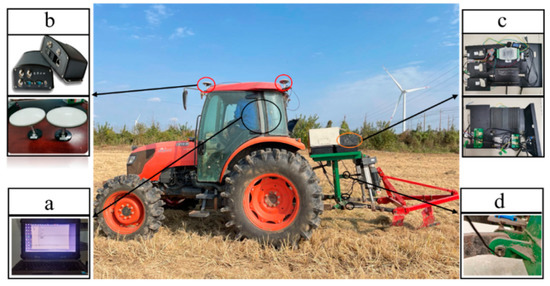
Figure 1.
Data acquisition platform. (a) Host computer; (b) P3-DT BeiDou navigation system; (c) controller; (d) shaft pin sensor. The position indicated by the arrow in (d) is the three-point hitch upper link at the back end.
2.3. Construction of the Identification Model
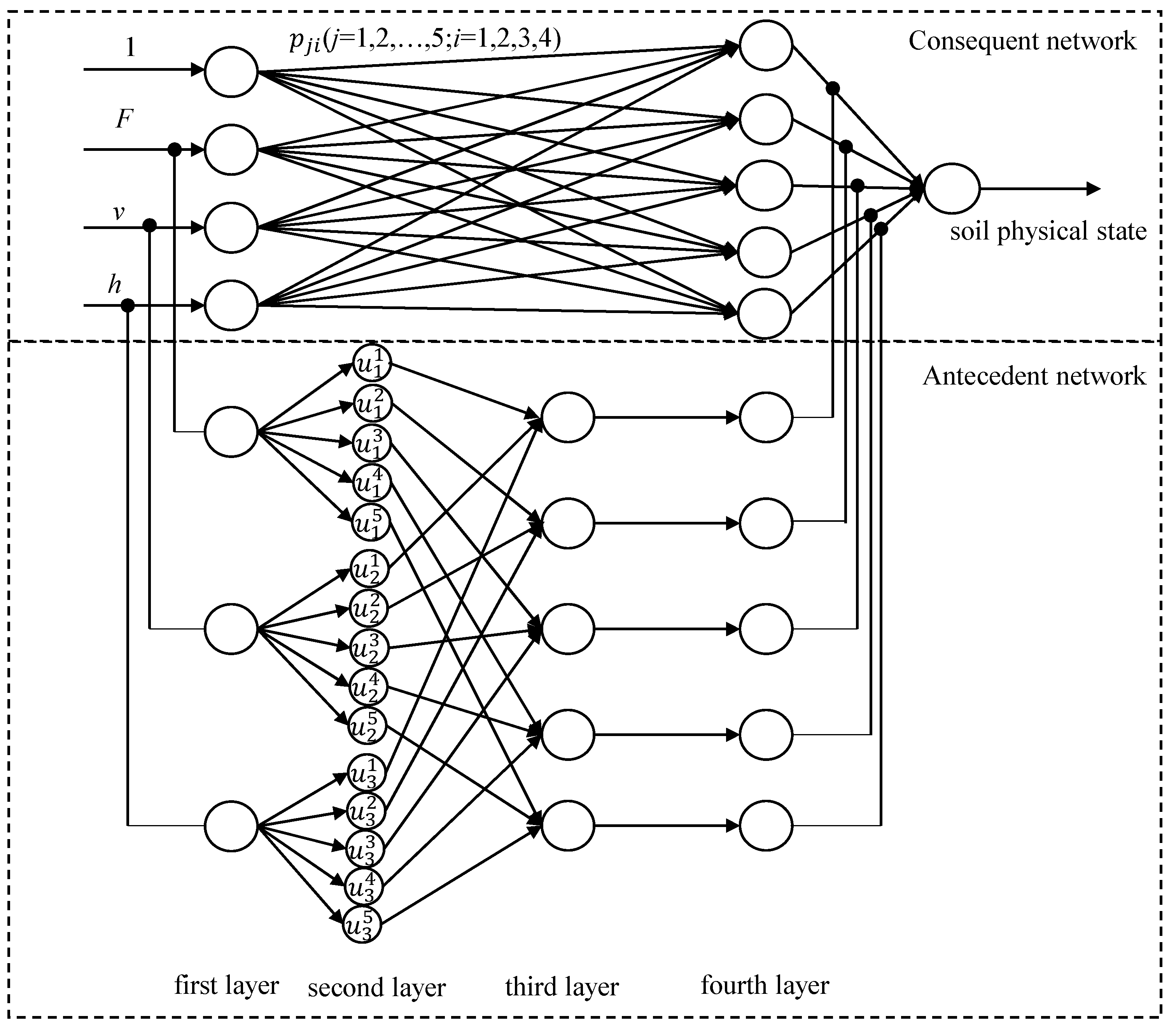
The Takagi–Sugeno (T–S) fuzzy neural network using the plowing parameters (traction resistance F, operation speed v, and plowing depth h) and soil physical state as the input and output of the model, respectively, is shown in Figure 2. The model is composed of a fuzzy model (antecedent network) and a neural network (consequent network). The organic combination of the fuzzy model and neural network broadens the range and ability of the neural network to process information, and the fuzzy relationship between the soil and the mechanical farming system can be effectively handled.

Figure 2.
Structure of the soil physical state perception model.
2.3.1. Antecedent Network
The first layer: The total number of nodes in this layer is N1 = n. Each neuron node is directly connected to the component of the input variable T and transmits each input value to the next layer.
The second layer: There are nodes in this layer. Each node denotes a fuzzy quantity, and its function is to calculate the membership function value of each input component belonging to its fuzzy quantity. The Gaussian function is used as its membership function, as shown in Formula (1).
where and are the center value and width value of the selected Gaussian membership function, respectively; i = 1, 2, 3, 4, j = 1, 2, 3… , i is the total dimension of the input variable; and is the total number of fuzzy segments of the input component.
The third layer: Each node in this layer shows a rule, and the total number of nodes is N3 = m, which is used to match the antecedents of fuzzy rules and calculate the applicability of each rule, as shown in Equation (2).
where ,,…, , , j = 1, 2, …, m; m = .
The fourth layer: This layer normalizes the applicability of the third layer, and the total number of nodes is N4 = m, that is:
2.3.2. Consequent Network
The first layer: This layer is the input layer. The value of the first node (x0) is 1 and it provides a constant term for the calculation of fuzzy rules in the consequent network.
The second layer: Each node in this layer means a rule and is used to calculate the consequent, that is:
The third layer: This layer is the output layer of the model, that is:
2.4. Learning Optimization Algorithm
The parameters need to be initialized and optimized in the prediction model and include the fuzzy segmentation numbers of input data, the center value , and width value of the membership function of the antecedent network and the connection weight coefficient of the consequent network. In this paper, fuzzy c-means clustering based on subtractive clustering is used to identify the number of fuzzy segmentation, the central value , and width values The hybrid learning algorithm is used to optimize the connection weight coefficient, the central value and width value .
2.4.1. Clustering Algorithm for the Parameter Identification of the Antecedent Network
Compared with FCM, the fuzzy C-means clustering algorithm based on subtraction clustering combines SCM (Subtractive Clustering Method) and FCM and solves the problems of sensitivity to initial value setting and slow training speed in the antecedent network structure and improves the speed and accuracy of model parameter identification. If dataset X is divided into c classes and the membership degree of each sample j belonging to a certain class i is , then the steps of the fuzzy C-means clustering method based on subtractive clustering are as follows:
- (1)
- Initialization: Using the SCM method to initialize the model input data center value , i = 1, 2, …, c.
- (2)
- Calculate the membership degree of each sample j belonging to the sample data center value , and the constraint condition is .
- (3)
- Recalculate the center value of the model input data:
- (4)
- Calculate the value of the objective function:
- (5)
- After completing a cycle, compare the value of the objective function until the numerical convergence stop iteration.
According to the clustering results, the number of clustering centers is the fuzzy segmentation number, and the initial values of the center value and width value are set by the membership relationship of the sample data belonging to the clustering center.
2.4.2. Hybrid Learning Algorithm for Parameter Optimization
When the hybrid learning algorithm propagates forward, the node parameters are used to calculate the output of the antecedent network, and the connection weight coefficient is updated by using the least square method. When propagating backward, the center value and width value of the membership function are optimized by the gradient descent method.
The error cost function E of the model is expressed as follows:
where t and y are the target value and the actual value, respectively.
The expression of connection weight coefficient:
Then the connection weight coefficient can be calculated using the sequence in Formula 12 derived by the least square method [23]:
where is the matrix composed of the ith row element of matrix A composed of connection weight coefficients, is the ith element of matrix B composed of the second layer of the subsequent network, X is the matrix composed of input data, and is the covariance matrix.
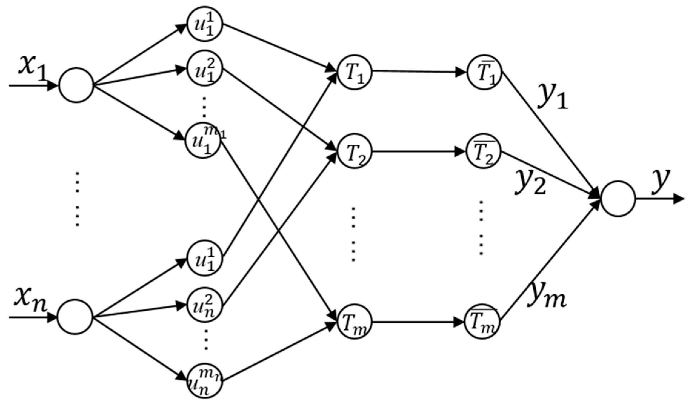
Figure 3 is a simplified form of a single-output fuzzy neural network (Figure 2). For the jth node of the q layer in the fuzzy neural network structure, let the input and output of the layer network be and , respectively. Therefore, the function of each layer node in the neural network structure in Figure 3 is expressed as follows:

Figure 3.
Simplified neural network structure.
The first layer:
The second layer:
The third layer:
The fourth layer:
The fifth layer:
Calculate , by chain rule and use the gradient descent method to optimize , .
If is an input of the jth fuzzy rule node of the model, then:
else:
Similarly, the first-order gradient of the error cost of is as follows:
Therefore, the algorithm of the parameter gradient descent propagation learning optimization is:
where is the learning rate and .
2.5. Overview of Experimental Field
In October 2021, a plowing experiment was conducted at the Shanghai Farm (N33°29.0673′, E120°55.899′) in the Dafeng District, Yancheng City, Jiangsu Province. This area belongs to the northern subtropical monsoon climate. The soil type is mainly clay soil, the previous crop is rice, the surface cover crop is stubble and straw, and the crushing length of the straw is approximately 10 cm. During the test, the average high temperature was 25 °C, and the average wind level was level 2.
2.6. Test Method
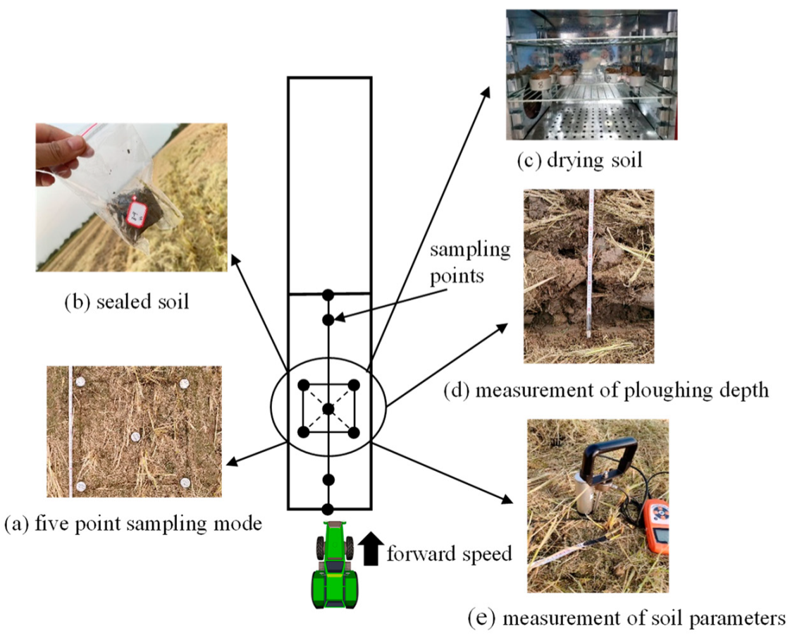
To ensure sufficient data items and improve the generalization capability of the neural network, we used a controllable variable plowing depth and working velocity based on different gradients. The plowing velocity gradients were 1.0 m/s, 1.2 m/s, 1.4 m/s, and 1.6 m/s, and the plowing depth gradients were 16 cm, 20 cm, and 24 cm. Detailed experiments were conducted 12 times, and each experiment was divided into separate sites, and 60 data samples were performed. The cone penetration resistance, soil volumetric moisture content, and plowing depth were measured using TJSD-750-II (Zhejiang topu yunnong Technology Co., Ltd., Hangzhou, China), TZS-1K-G (Zhejiang topu yunnong Technology Co., Ltd.), and a tape ruler, respectively, at each sampling point, as shown in Figure 4d,e. The distance between the sampling points is the product of the forward speed at the current level and the sampling module cycle at the current level. The same test operation was carried out every two days after the test site had been compacted using a tractor to ensure the accuracy of the cone penetration resistance and volumetric moisture content information. The same operation was performed a total of 12 × 4 = 48 times at different test sites using the above method. A schematic diagram of the test process is shown in Figure 4. It was not possible to keep the operating speed and plowing depth constant at any time owing to the effect of the complex environment of the field; however, the operating speed and plowing depth were kept as consistent as possible with the experimental design parameters through the operation of agricultural machinery drivers.

Figure 4.
Diagram of the soil parameter acquisition process.
To reduce the systematic error of the soil moisture meter and drift during detection, we randomly selected 10 points from each of the 60 sampling points, and a total of 10 × 12 = 120 soil in-situ samples were used to correct the soil moisture data at the corresponding position of the soil moisture meter. The five-point sampling mode was used to collect in-situ soil samples, as shown in Figure 4a. The width of sampling is 60 cm, and the length is the distance between sampling points. The collected soil samples were immediately packaged in a separate polyethylene bag after weighing, as shown in Figure 4b. After the test, the samples were dried for 12 h in an oven at 105 ± 1 °C, as shown in Figure 4c, and a constant weight was obtained. After drying, the soil moisture content of the sample was calculated and compared with the soil volumetric moisture content measured using the soil moisture meter.
The soil moisture content measured using a soil moisture meter is the soil volumetric moisture content, which is converted into soil moisture content using Equation (23).
where is the soil volume moisture content, is the soil moisture content, is the soil dry density, m is the soil mass, and V is the ring cutter volume (in this study, V = 100 cm3).
3. Results and Discussion
The difference in soil physical state has a direct influence on the energy consumption of plowing. This shows that when plowing is carried out with fixed operating parameters, the consumed energy can reflect the soil’s physical state. However, due to the complexity of soil structure, we can only select the key soil parameters that affect energy consumption to describe the soil’s physical state. Based on the above understanding, this paper obtains the traction resistance and operation speed in the process of plowing by installing shaft pin sensors and GPS on the data acquisition platform, and the plowing depth, cone penetration, and soil moisture content are measured by a tape ruler, soil compaction meter, and water content meter. The obtained operating parameters and soil parameters are used as the data basis for identifying the soil state in the soil–mechanical contact system. In order to describe the soil conditions during plowing, the soil’s physical state was divided into ‘soft’, ‘zero’, and ‘hard’ by the FCM algorithm with soil moisture content and cone penetration. The T–S fuzzy neural network classifier was constructed using traction resistance, operating velocity, and plowing depth and the three soil physical states as inputs and output, respectively, to indirectly identify the soil physical state. In the model, the fuzzy C-means clustering method based on subtractive clustering is used to determine the initial values of the antecedent network and the consequent network, and the hybrid learning algorithm based on the least square method and gradient descent method is used to optimize the initial values of the antecedent network and the consequent network, and finally, the model parameters are determined. The fuzzy rules in the neural network reflect the relationship between the operating parameters and the soil’s physical state, and it also guides the adjustment of the operating parameters during plowing; for example, if F is cluster1 (NB), v is cluster1 (PB), and h is cluster1 (NS), then y = 1 (soft).
3.1. Test Platform
Figure 1 shows the overall layout of the data acquisition platform. Providing sufficient data is necessary for statistical analysis, and a test platform is used for data collection. Taniguchi [24] measured the plowing speed from 0.07 m/s to 4.8 m/s using a soil bin and dynamometer car, which increased the difficulty of the experiment owing to the limitations of soil grooves. In this study, we used sensors to measure the plowing resistance, similar to the approach used by Shafaei [25] and Al-Suhaibani [26]. However, the data acquisition platform shown in Figure 1 is an independent unit and does not require the integration of other devices. Furthermore, the data acquisition platform has an independent control unit, which is convenient for other experiments, such as the use of the adjustment method for the plowing depth.
3.2. Draft Force and Soil Moisture Content
Figure 5 shows the soil moisture content at plowing depths of 16 cm and 24 cm. The average soil moisture content decreased by 4.1% when the plowing depth increased from 16 cm to 24 cm, indicating that the soil moisture content decreased with the increase in paddy soil depth, which is not consistent with the results reported by Ji [27]. This is because the bare surface accelerates the evaporation of surface soil moisture after harvesting rice. In addition, at plowing depths of 16 cm and 24 cm, the maximum change values of the adjacent acquisition points were 11.6% and 14.5%, respectively. The change form of the soil moisture content in the horizontal and vertical directions indicates that soil moisture content has spatial differences, which agrees with the results reported by Brocca [28]. The spatial difference in soil moisture content is also one of the main reasons for the change in the traction resistance. Sahu [29] reported similar conclusions.
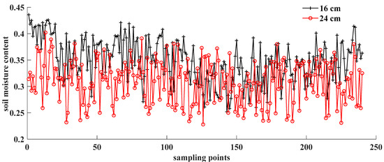
Figure 5.
Soil moisture content at tillage depths of 16 cm and 24 cm.
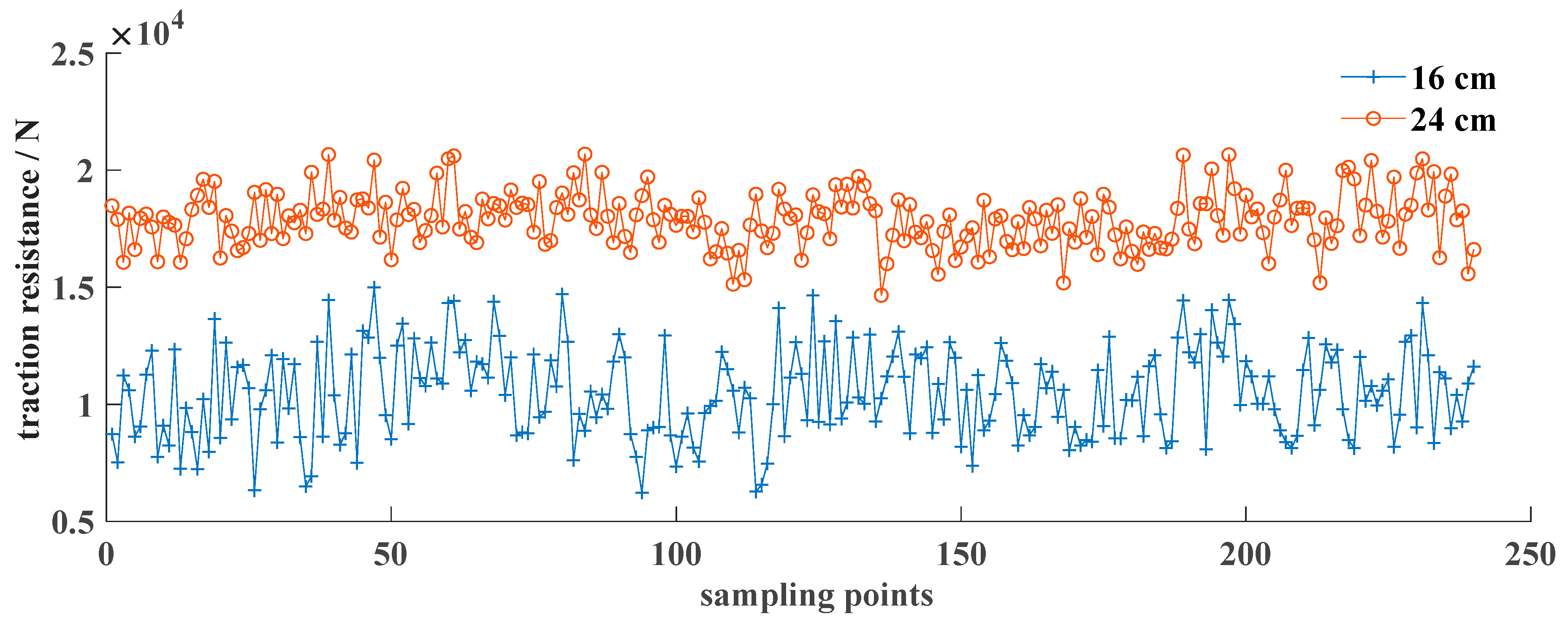
Figure 6 shows the traction resistance at plowing depths of 16 cm and 24 cm. At a plowing depth of 16 cm, the variation range of the traction resistance was larger, which is similar to the result obtained by Nassir [30]. This is due to the combined effect of agricultural machinery harvesting operations on surface soil compaction and natural weather. Compared with the traction resistance measured in the study by Alwan [31], the traction resistance measured in this study is larger, which is closely related to mechanical rolling during harvesting in paddy soil. However, the trend of the change in data is consistent with that in the study by Alwan [31].
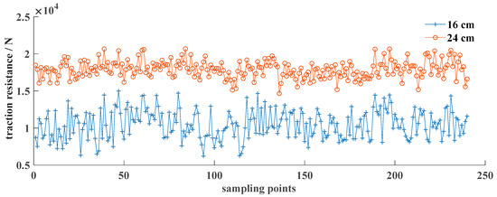
Figure 6.
Traction resistance at tillage depths of 16 cm and 24 cm.
3.3. Soil Physical State
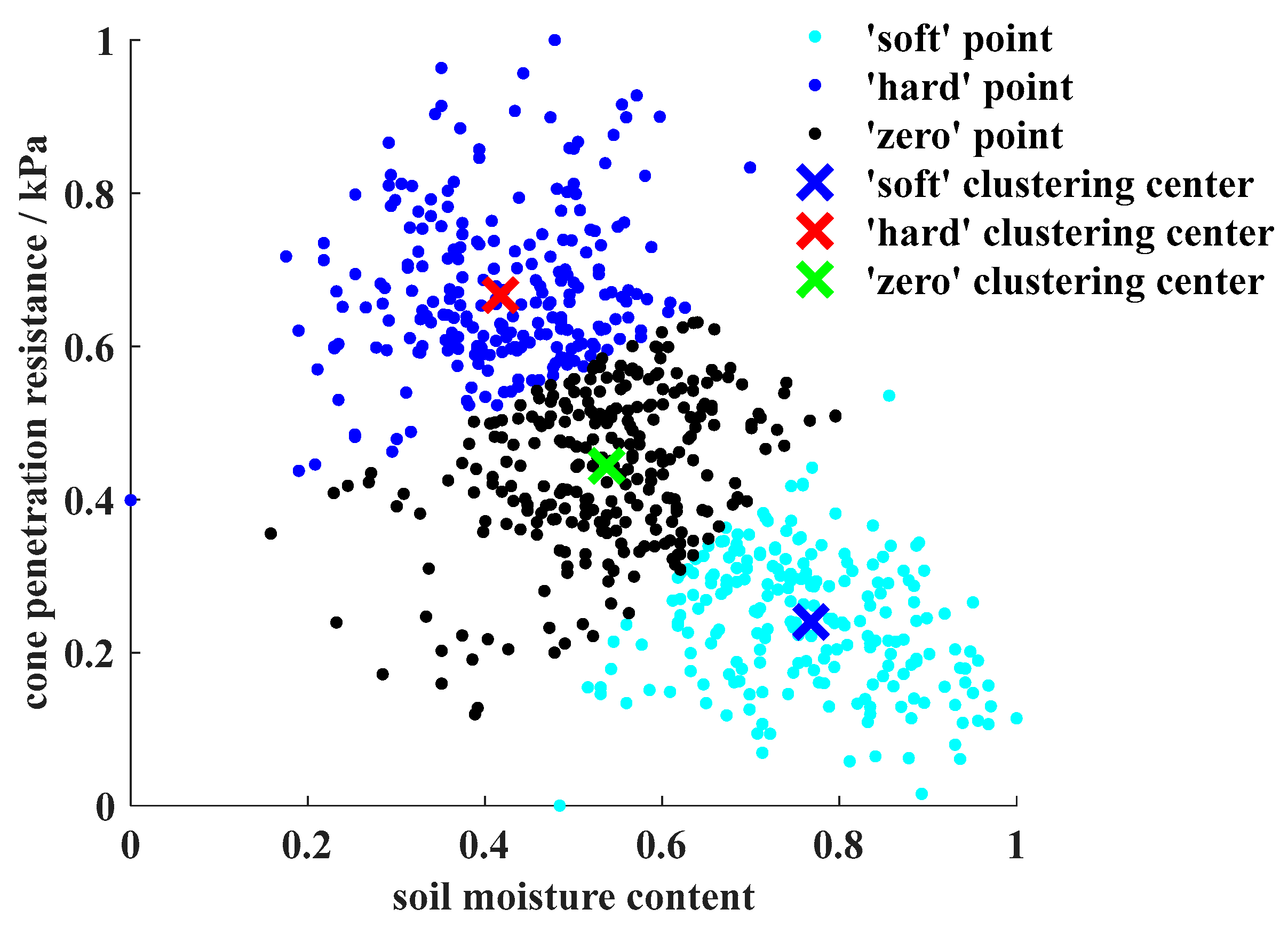
As an influencing factor in the soil–tool contact system, soil directly affects the traction resistance in the process of plowing. In this study, we considered the soil physical characteristics that affect traction resistance based on the principle of the identification model. However, there are many soil factors that affect traction resistance. In this study, soil cone penetration resistance and moisture content were selected as indicators to classify the soil’s physical state, which is useful for the real-time application of the model. Considering the dimensional difference between soil cone penetration resistance and moisture content, 720 data sets were normalized and clustered using the FCM method. The membership relationship between the sample data and each evaluation grade was extracted to establish the soil physical state of each sample data set. The clustering results of 720 sample data sets are shown in Figure 7. In the 720 groups of two-dimensional information arrays, the values of the first, second, and third cluster centers (‘soft’, ‘zero’, and ‘hard’) are 214, 272, and 234, respectively, indicating that the classification of the soil physical state using cone penetration resistance and soil moisture content can yield better discrimination. The clustering results showed that the soil in the experimental plot exhibited a complex mixed state after harvesting rice, which further demonstrates the importance of adjusting the operating parameters according to the soil state.

Figure 7.
Clustering results of the soil’s physical state.
3.4. Clustering Algorithm
In this study, the soil conditions were classified into ‘hard’, ’zero’, and ‘soft’, three physical states, using the FCM, taking soil moisture content and cone penetration resistance as the indexes. Compared with the K-means clustering, FCM is more suitable for the complex structure of soil itself. This advantage is reflected in the fact that soil physical parameters are continuous; K-means has poor clustering performance when the data points belonging to different categories (soil physical parameters) are close. For the FCM algorithm, the criteria for judging the data points belonging to different categories are determined by the degree of membership, which makes it possible to analyze the data points with different categories by the degree of membership when the data points are close. The authors of [32] show the same conclusion.
3.5. Perception Model
3.5.1. Datasets
According to the results of the plowing experiment in Section 2.6 and the division of soil physical state in Section 3.3, 720 datasets of traction resistance, working parameters (operating speed and plowing depth), and corresponding data sets of soil physical state were obtained after processing the experimental data. In the 720 data sets, the number of soil groups under ‘soft’, ‘zero’, and ‘hard’ conditions was 214, 272, and 234, respectively. Considering that the output of the T–S fuzzy neural network is an accurate value, the ‘soft’, ‘zero’ and ‘hard’ soil physical states correspond to the values 1, 2, and 3 respectively.
To verify the prediction accuracy of the model, we used the Neuro-Fuzzy Designer toolbox in MATLAB R2017b and the manually coded fuzzy C-means clustering based on subtractive clustering to simulate 440 training sets and 280 test sets. The number of ‘soft’, ‘zero’, and ‘hard’ states in the training set and test set must be as close as possible, which can reduce the training error of the model. After 100 times of training, the number of soft, real, and hard soil in the 440 training sets and 280 test sets was 128, 172, and 140 and 86, 100, and 94, respectively, which can meet the accuracy requirements of model training.
3.5.2. Parameter Settings
The algorithm in Section 2.4 is used to optimize the parameters of the T–S fuzzy neural network model. The fuzzy segmentation numbers of fuzzy variables F, v, and h are m1 = m2 = m3 = 5. Each layer number of the neural network is N1 = n = 3, N2 = 15, and N3 = N4 = 5, respectively. The subtractive clustering radius is , and the threshold is .
3.5.3. Training Environment
To set the neural network model, an ASUS G512L with an Intel® Core™ i7-10870 H CPU @ 2.20 GHz, NVIDIA GeForce RTX 2060, 16 GB RAM notebook computer running MATLAB R2017b software (Natick, America) was used. After the training, we used more data to test the model and 0.5 s was required to obtain results.
3.5.4. Algorithm Comparison
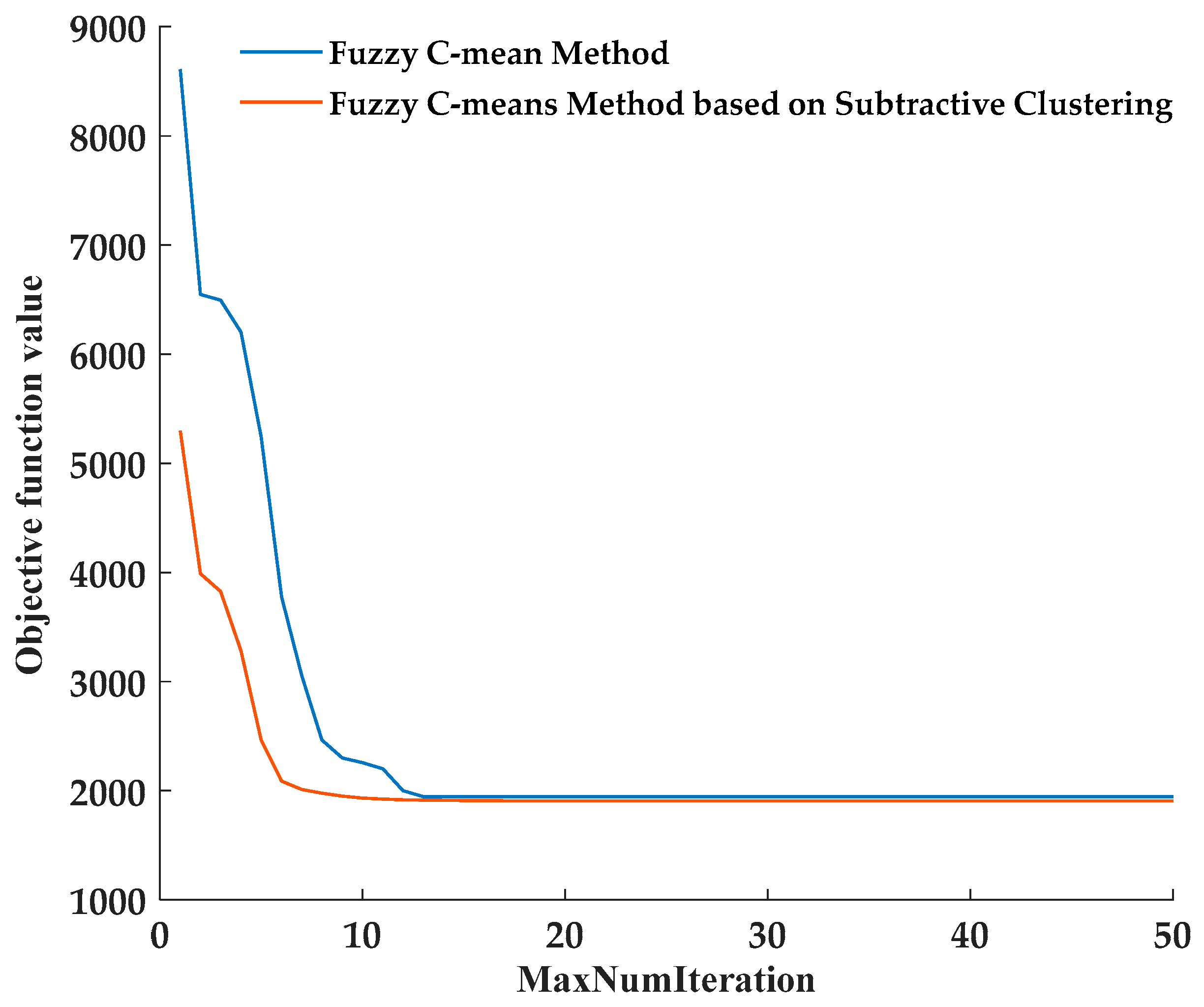
In order to solve the problem of fuzzy C-means clustering being sensitive to the set value in identifying the parameters of the antecedent network, the fuzzy C-means clustering method based on subtractive clustering was selected for optimizing the model, and the robustness of the model was improved by reducing the number of hyper-parameters. Both algorithms are clustering methods based on objective function optimization, and the response speed of the algorithm can be judged by the change of the objective function in the iteration process. The change of the objective function with the number of iterations is shown in Figure 8.

Figure 8.
Comparison of the objective function changes.
The fuzzy C-means clustering based on subtractive clustering has reached a relatively stable state when iterating the sixth time, and the subtractive clustering only appears in this state when iterating 13 times. In addition, due to the different super-parameter settings, the clustering centers are different, resulting in a large difference in the initial value of the objective function. We also found that when the number of clusters set is different from the number of fuzzy C-means clustering based on subtractive clustering, the solutions found by the two are quite different. In reverse, the calculation results are basically the same, but the number of iterations of fuzzy C-means clustering based on subtractive clustering is less than that of FCM. This is the same as the conclusion of [33]. The roles of FCM and fuzzy C-means clustering algorithm based on subtractive clustering in the study are shown in Table 1.

Table 1.
Functions of the clustering algorithm.
The fuzzy C-means clustering method based on subtractive clustering was used to identify the parameters of the antecedent network. Precision, Recall, and F-score are used as evaluation indexes, and the gradient descent (GD), hybrid learning algorithm (Hybrid), and genetic algorithm [34] (GA) are used for the parameter optimization of the consequent network, respectively. The evaluation indexes are compared, as shown in Table 2, where the response time is the delay time.
Table 2.
Comparison of evaluation index results.
According to the results in Table 2, although the response speed of the GD model is better than Hybrid and GA, the Precision, Recall, and F-score of the model cannot meet the requirements. At the same time, the evaluation indexes of the GA model are 1.45%, 1.67%, and 3.15% higher than those of Hybrid, respectively, but the model takes 0.33 s more. For the application of this model, when the evaluation index values are similar, the response speed is very important, which directly affects the field operation. Therefore, Hybrid is more suitable for the optimization of subsequent network parameters in this study.
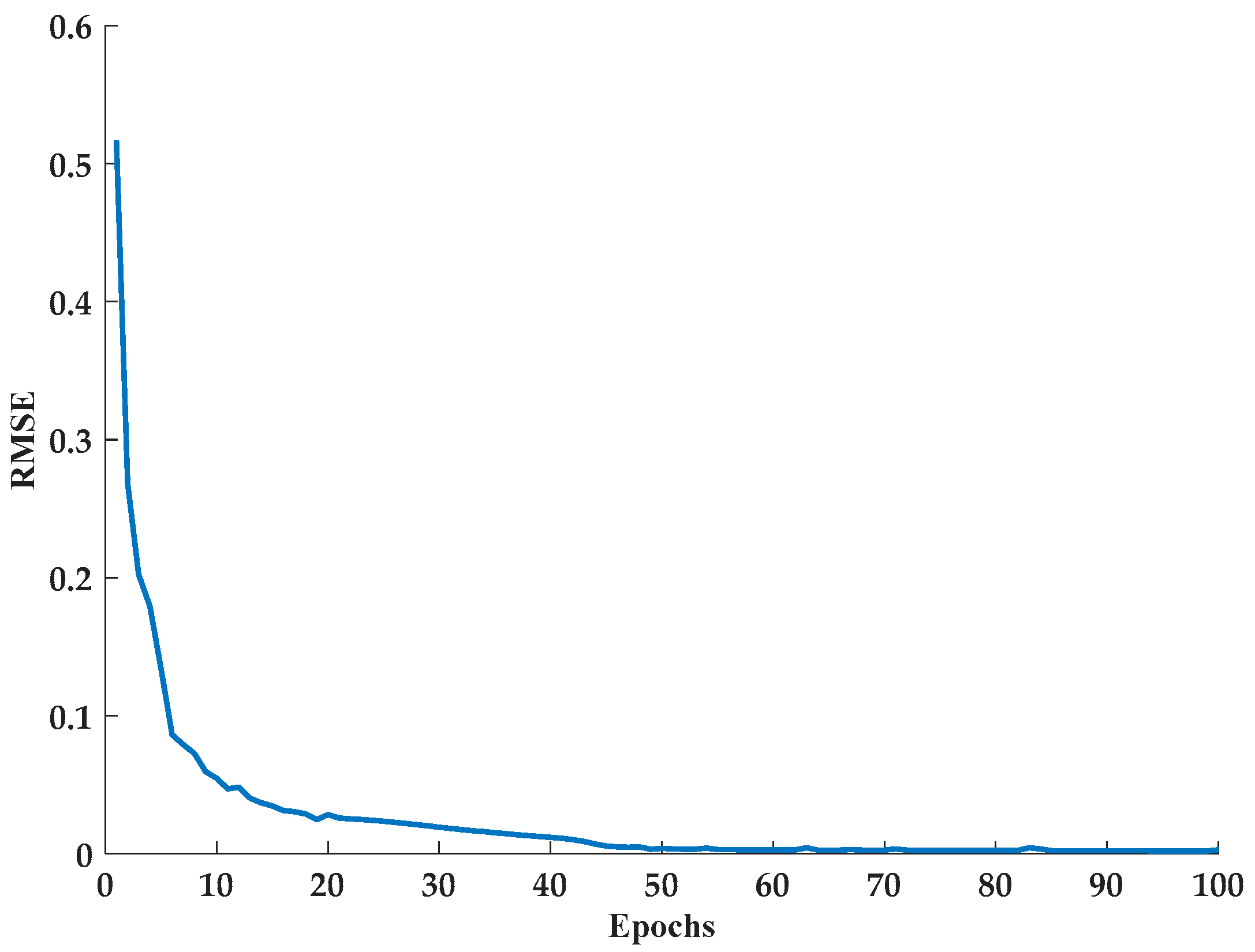
The fuzzy C-means clustering method based on subtractive clustering and the hybrid learning algorithm were used to identify the network structure parameters of the antecedent and the optimization model parameters, respectively. The training results of 240 validation sets are shown in Table 3, and the RMSE variation curve of the model is shown in Figure 9. Table 3 shows that the prediction model of the soil physical state trained using 440 data sets yielded 264 correct groups and the Accuracy, Precision, Recall, and F-Score are 94.29%, 94.41%, 94.56%, and 93.05%, respectively when 280 test data sets were predicted. Among the 94 groups of ’hard’ state real results, five groups of ’zero’ state prediction results were obtained; the prediction results of nine ‘hard’ states and two ‘soft’ states belong to 100 ‘zero’ states; and 86 groups of ‘soft’ states were accurately predicted. As the epochs increase, RMSE decreases from the initial value of 0.52 to 0.01 when the number of epochs reaches 30, which can be found in Figure 9. It can be observed that the prediction results obtained using the T–S fuzzy neural network model are essentially consistent with the actual situation, indicating that the model can accurately and effectively predict the soil’s physical state during tractor plowing in the field.
Table 3.
Confusion matrix of the prediction results.
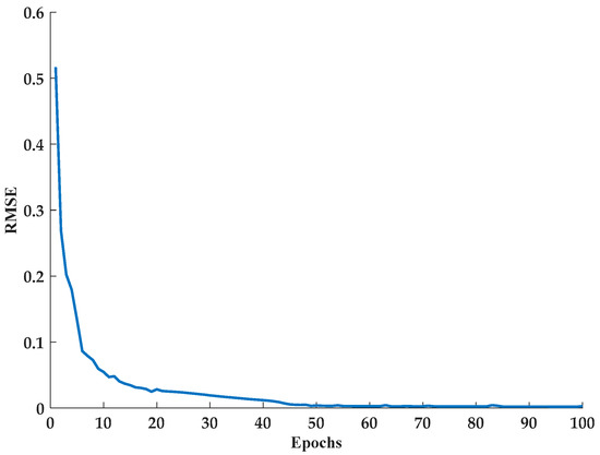
Figure 9.
Model training results.
The studies in [35,36] used a neural network mainly for predicting the traction resistance and plowing energy consumption in a soil–mechanical contact system. Few studies have been conducted on the use of a soil condition identification model during the plowing process, which is necessary for adjusting the parameters in the operation process. This study focused on identifying the soil conditions in the plowing operation process, and good results were obtained. The fuzzy C-means clustering method based on subtractive clustering was used to identify the structural parameters of the fuzzy neural network. Compared with the method used in [34], although the calculation results of the genetic algorithm are better than those of the clustering algorithm, the algorithm used in this paper shows advantages in response speed, which is also an important issue to be considered in the plowing process. The results can be obtained after about 0.5 s. Although there is a certain delay, the tractor driving distance in the delay process is less than the distance of the sampling point in the test process. Therefore, the existence of this delay is acceptable. In summary, this study focused on identifying the soil conditions in the plowing operation process, and good results were obtained.
4. Conclusions
- (1)
- Complex and unclear relationships exist between plowing resistance, working parameters, and soil conditions. In this study, the field operation parameters and soil physical parameters were obtained using a data acquisition platform and soil instrument to construct the T–S fuzzy neural network for predicting soil physical state.
- (2)
- We measured soil moisture content corresponding to working parameters during plowing. The average soil moisture content decreased by 4.1% when the plowing depth increased from 16 cm to 24 cm, indicating that the soil moisture content decreased with the increase in paddy soil depth. In addition, at plowing depths of 16 cm and 24 cm, the maximum change values of the adjacent acquisition points were 11.6% and 14.5%, respectively. The change form of the soil moisture content in the horizontal and vertical directions indicates that soil moisture content has spatial differences.
- (3)
- The T–S fuzzy neural network classifier was constructed using traction resistance, operating velocity, and plowing depth as inputs and the soil’s physical state as output. Our results show that when 280 groups of test data were used to verify the model, 264 groups were accurately predicted, and the Accuracy, Precision, Recall, and F-Score of the fuzzy model are 94.29%, 94.41%, 94.56%, and 93.05%. This indicates that the T–S fuzzy neural network model based on plowing resistance and working parameters can accurately identify the physical state of paddy soil in real-time during plowing, which provides a reliable reference for the selection of the optimal combination of plowing parameters and reduction in the energy consumption, thereby improving the overall efficiency of plowing.
- (4)
- Based on the conclusions of this paper, the optimal combination of operating parameters under different soil physical states can be further studied using DEM.
Author Contributions
Conceptualization, J.Z. (Jianlei Zhao) and J.Z. (Jun Zhou); methodology, J.Z. (Jianlei Zhao); software, X.W. and Z.Q.; validation, Z.L. and C.S.; formal analysis, J.Z. (Jianlei Zhao); investigation, Z.Q.; resources, J.Z. (Jun Zhou); data curation, Z.L.; writing—original draft preparation, J.Z. (Jianlei Zhao); writing—review and editing, J.Z. (Jianlei Zhao) and C.S.; visualization, X.W.; supervision, J.Z. (Jun Zhou); project administration, J.Z. (Jun Zhou); funding acquisition, J.Z. (Jun Zhou). All authors have read and agreed to the published version of the manuscript.
Funding
This research was funded by Jiangsu Province Policy Guidance Project (North Jiangsu Science and Technology Special Project) (SZ-LYG202011) and National Key Research and Development Project (2019YFD0900701).
Institutional Review Board Statement
Not applicable.
Informed Consent Statement
Not applicable.
Data Availability Statement
Not applicable.
Acknowledgments
The authors would like to thank the anonymous reviewers for their kind suggestions and constructive comments. We thank the Shanghai Farm support in conducting the experiment.
Conflicts of Interest
The authors declare there is no conflict of interest.
References
- Xie, B.; Wu, Z.B.; Mao, E.R. Development and Prospect of Key Technologies on Agricultural Tractor. Trans. Chin. Soc. Agric. Mac. 2018, 49, 1–17. [Google Scholar]
- Ibrahmi, A.; Bentaher, H.; Hbaieb, M.; Maalej, A.; Mouazen, A.M. Study the effect of tool geometry and operational conditions on mouldboard plough forces and energy requirement: Part 1. Finite element simulation. Comput. Electron. Agric. 2015, 117, 258–267. [Google Scholar] [CrossRef]
- Soni, P.; Salokhe, V.M.; Nakashima, H. Modification of a mouldboard plough surface using arrays of polyethylene protuberances. J. Terramech. 2007, 44, 411–422. [Google Scholar] [CrossRef]
- Owende, P.M.O.; Ward, S.M. Characteristic loading of light mouldboard ploughs at slow speeds. J. Terramech. 1996, 33, 29–53. [Google Scholar] [CrossRef]
- Panigrahi, B.; Mishra, J.N.; Swain, S. Effect of implement and soil parameters on penetration depth of a disc plow. AMA 1990, 21, 9–12. [Google Scholar]
- Kheiralla, A.F.; Yahya, A.; Zohadie, M.; Ishak, W. Modelling of power and energy requirements for tillage implements operating in Serdang sandy clay loam, Malaysia. Soil Tillage Res. 2004, 78, 21–34. [Google Scholar] [CrossRef]
- Qiong, G.; Pitt, R.E.; Ruina, A. A model to predict soil forces on the plough mouldboard. J. Agric. Eng. Res. 1986, 35, 141–155. [Google Scholar] [CrossRef]
- Hettoaratchi, D.R.P. Predicting the draught requirements of concave agricultural discs. J. Terramech. 1997, 34, 209–224. [Google Scholar] [CrossRef]
- Manuwa, S.I.; Ademosun, O.C. Draught and Soil Disturbance of Model Tillage Tines Under Varying Soil Parameters. CIGR J. 2007, 9, 1–17. [Google Scholar]
- Shafaei, S.; Loghavi, M.; Kamgar, S. A comparative study between mathematical models and the ANN data mining technique in draft force prediction of disk plow implement in clay loam soil. CIGR J. 2018, 20, 71–79. [Google Scholar]
- Abd El Wahed, M.A. Draft models of chisel plow based on simulation using artificial neural networks. Misr J. Agr. Eng. 2007, 24, 42–61. [Google Scholar]
- Akbarnia, A.; Mohammadi, A.; Alimardani, R.; Farhani, F. Simulation of draft force of winged share tillage tool using artificial neural network model. CIGR. J. 2014, 16, 57–65. [Google Scholar]
- Alimardani, R.; Abbaspour-Gilandeh, Y.; Khalilian, A.; Keyhani, A.; Sadati, S.H. Prediction of draft force and energy of subsoiling operation using ANN model. J. Food. Agric. Environ. 2009, 7, 537–542. [Google Scholar]
- Al-Hamed, S.A.; Wahby, M.F.; Al-Saqer, S.M.; Aboukarima, A.M.; Sayedahmed, A.A. Artificial neural network model for predicting draft and energy requirements of a disk plow. J. Anim. Plant Sci. 2013, 23, 1714–1724. [Google Scholar]
- Shafaei, S.M.; Nourmohamadi-Moghadami, A.; Kamgar, S. Development of artificial intelligence based systems for prediction of hydration characteristics of wheat. Comput. Electron. Agric. 2016, 128, 34–45. [Google Scholar] [CrossRef]
- Sefeedpari, P.; Rafiee, S.; Akram, A.; Komleh, S.H.P. Modeling output energy based on fossil fuels and electricity energy consumption on dairy farms of Iran: Application of adaptive neural-fuzzy inference system technique. Comput. Electron. Agric. 2014, 109, 80–85. [Google Scholar] [CrossRef]
- Chi, R.; Li, H.; Shen, D.; Huang, B. Enhanced P-type Control: Indirect Adaptive Learning from Set-point Updates. IEEE Trans. Autom. Control 2022. [Google Scholar] [CrossRef]
- Roman, R.C.; Precup, R.E.; Petriu, E.M. Hybrid data-driven fuzzy active disturbance rejection control for tower crane systems. Eur. J. Control 2021, 58, 373–387. [Google Scholar] [CrossRef]
- Godwin, R.; O’dogherty, M.J.; Saunders, C.; Balafoutis, A.T. A force prediction model for mouldboard ploughs incorporating the effects of soil characteristic properties, plough geometric factors and ploughing speed. Biosyst. Eng. 2007, 97, 117–129. [Google Scholar] [CrossRef]
- Godwin, R.J.; O’Dogherty, M.J. Integrated soil tillage force prediction models. J. Terramech. 2007, 44, 3–14. [Google Scholar] [CrossRef]
- Desbiolles, J.M.A.; Godwin, R.J.; Kilgour, J.; Blackmore, B.S. Prediction of tillage implement draught using cone penetrometer data. J. Agric. Eng. Res. 1999, 73, 65–76. [Google Scholar] [CrossRef]
- Li, R.X.; Gao, H.W.; Su, Y.S. Effect of Soil Bulk Density and Moisture Content on the Draft Resistance. Trans. Chin. Soc. Agric. Eng. 1998, 14, 81–85. [Google Scholar]
- Jang, J.R. ANFIS: Adaptive-network-based fuzzy inference system. IEEE Trans. Syst. Man Cybern. 1993, 23, 665–685. [Google Scholar] [CrossRef]
- Taniguchi, T.; Makanga, J.T.; Ohtomo, K.; Kishimoto, T. Draft and soil manipulation by a moldboard plow under different forward speed and body attachments. Trans. ASAE 1999, 42, 1517. [Google Scholar] [CrossRef]
- Shafaei, S.M.; Loghavi, M.; Kamgar, S. Appraisal of Takagi-Sugeno-Kang type of adaptive neuro-fuzzy inference system for draft force prediction of chisel plow implement. Comput. Electron. Agric. 2017, 142, 406–415. [Google Scholar] [CrossRef]
- Al-Suhaibani, S.A.; Ghaly, A.E. Effect of plowing depth of tillage and forward speed on the performance of a medium size chisel plow operating in a sandy soil. Am. J. Agric. Biol. Sci. 2010, 5, 247–255. [Google Scholar] [CrossRef]
- Ji, R.H.; Li, X.; Zhang, S.L.; Zheng, L. Prediction of soil moisture in multiple depth based on time delay neural network. Trans. Chin. Soc. Agric. Eng. 2017, 33, 132–136. [Google Scholar]
- Brocca, L.; Melone, F.; Moramarco, T.; Morbidelli, R. Spatial-temporal variability of soil moisture and its estimation across scales. Water Resour. Res. 2010, 46, 1–14. [Google Scholar] [CrossRef]
- Sahu, R.K.; Raheman, H. Draught prediction of agricultural implements using reference tillage tools in sandy clay loam soil. Biosyst. Eng. 2006, 94, 275–284. [Google Scholar] [CrossRef]
- Nassir, A.J. Effect of moldboard plow types on soil physical properties under different soil moisture content and tractor speed. Basrah J. Agric. Sci. 2018, 31, 48–58. [Google Scholar] [CrossRef]
- Alwan, A.A. A Field Study of Soil Pulverization Energy by using Different Moldboards Types Under Various Operating Condition. Basrah J. Agric. Sci. 2019, 32, 373–388. [Google Scholar] [CrossRef]
- Vernieuwe, H.; De, B.B.; Verhoest, N.E.C. Comparison of clustering algorithms in the identification of Takagi–Sugeno models: A hydrological case study. Fuzzy Sets Syst. 2006, 157, 2876–2896. [Google Scholar] [CrossRef]
- Li, P. Study on Fuzzy Identification Methods for Nonlinear Systems Based on T-S Model. Master’s Thesis, Jiangsu University, Zhenjiang, China, 10 June 2008. [Google Scholar]
- Siarry, P.; Guely, F. A genetic algorithm for optimizing Takagi-Sugeno fuzzy rule bases. Fuzzy Sets Syst. 1998, 99, 37–47. [Google Scholar] [CrossRef]
- Roul, A.K.; Raheman, H.; Pansare, M.S.; Machavaram, R. Predicting the draught requirement of tillage implements in sandy clay loam soil using an artificial neural network. Biosyst. Eng. 2009, 104, 476–485. [Google Scholar] [CrossRef]
- Al-Dosary, N.M.N.; Al-Hamed, S.A.; Aboukarima, A.M. Application of adaptive neuro-fuzzy inference system to predict draft and energy requirements of a disk plow. Int. J. Agric. Biol. Eng. 2020, 13, 198–207. [Google Scholar]


Publisher’s Note: MDPI stays neutral with regard to jurisdictional claims in published maps and institutional affiliations. |
© 2022 by the authors. Licensee MDPI, Basel, Switzerland. This article is an open access article distributed under the terms and conditions of the Creative Commons Attribution (CC BY) license (https://creativecommons.org/licenses/by/4.0/).