Simulation of Climate Change Impacts on Crop Yield in the Saskatchewan Grain Belt Using an Improved SWAT Model

Abstract

Climate change has a potentially significant influence on agricultural production in southern Saskatchewan. Crop yields are susceptible to weather patterns and seasonal fluctuations in this sub-humid region owing to the predominance of rain-fed farming practices. A modified Soil and Water Assessment Tool (SWAT-M) and the output from 10 high-resolution (0.22°) regional climate models (RCMs) were used to develop simulations of spring wheat and rain-fed canola in 296 rural municipalities (RM) for a historical baseline period (1975–2004) and three 30-year future periods: near (2010–2039), middle (2040–2069), and far (2070–2099). We combined SWAT-M with the S-curve method to adjust yield to the original drought stress in the source code and evaluated eight indices of extreme precipitation and temperature. Results of calibration and validation suggest that the simulated crop yields generally agree with observed data. Crop yield showed lesser performance compared with streamflow and soil water content (SWC) along with percent bias, ranging from −9.6% to −14.8%, while streamflow calibration ranges from −5.3% to −7.7%. The multi-model ensemble median showed increasing radiative forcing in the temperature and precipitation indices, such that the RCM-projected weather indices were found to be warmer and wetter than those estimated using regional historical data. The results of simulating canola and spring wheat indicate an increase in crop yield of 17% and 9.7% in the near future, 28.2% and 15.6% in the middle future, and 44.7% and 32% in the far future, respectively. Although, there has been an increase in the median wheat and canola yields, a significant reduction in the annual production is observed. This decline in yield amounts to around 1000 kg/ha and is anticipated to occur in the near and middle future. This trend is quite pronounced in the extreme south and southwest regions. Overall, this innovative research framework, along with the region-specific model outcomes in the form of crop yield projections, will aid in the formulation of future agricultural policies aimed at promoting effective climate adaptation strategies.

1. Introduction

Southern Saskatchewan contains approximately 42% of Canada’s cropland, where more than 32,000 farms produce canola and wheat [1]. According to Statistics Canada, wheat and canola production totaled 9.1 and 7.9 million tons, respectively in 2014. This region is the leading Canadian crop exporter with wheat exports of approximately CAD $2.2 million in 2014 [2,3]. However, agricultural production has fluctuated during recent times, primarily owing to the impacts of climate variability that dominate the entire prairie landscape and, in particular, southern Saskatchewan [4,5,6,7,8]. Climate change impacts include reducing soil water content, raising soil temperature, and causing a shift in seasonal variability and extreme weather, including the severity and frequency of droughts and excess water [9,10,11]. Clearly, crop yield simulation as affected by climate change is required to support decision- and policy-making on a regional scale.

Hydrological models can accurately capture above- and below-ground biomass characteristics to simulate crop production [12]. However, such predictive models require appropriate inputs and multi-step calibration [13]. The Soil and Water Assessment Tool (SWAT) model [14] has been used at various scales to simulate streamflow [15,16,17,18], soil water content [19,20,21,22,23], soil temperature [20,24], and sediment yield [25,26] around the world owing to its computational efficacy and its capability to forecast long-term effects [27]. Although this model is capable of simultaneously simulating average crop yield [12,28,29,30,31,32,33,34], only a handful of studies have used it to evaluate the impact of climate change on crop yield in Canada. Kang et al. [35] used three greenhouse gas (GHG) emission scenarios (Representative Concentration Pathways—RCP2.6, 4.5, and 8.5) in Atlantic Canada. Their results indicated a negative influence of climate change on the yields for potato and barley under the investigated RCP scenarios, with substantial drops (13–23%) in crop yields during 2060–2099 under RCP8.5. A comparable research work focusing on crops in the prairie region is non-existent despite the severe impacts of climate change.

The SWAT model’s incorporation of essential hydrological components, such as SWC, makes it highly advantageous for simulating crop yield. By accounting for complex interactions between soil moisture, water availability, and plant growth, the model provides a comprehensive understanding of the hydrological processes influencing crop productivity. Furthermore, the SWAT’s ability to simulate the dynamic variation in SWC and its impact on crop growth and water stress enables yield predictions under varying climatic and soil conditions. While the model has found wide applications in simulating various environmental parameters like streamflow, soil moisture, and crop yield, it encounters limitations in colder climate regions where streamflow is largely due to snowmelt during spring. Similarly, an algorithm calculates aeration stress (astrs) using the WRC of the entire soil profile and, as such, the model does not provide accurate estimates for plants with shallow roots such as wheat and canola. The main achievement of this undertaking is the successful coupling of a physically based soil temperature module, as opposed to an empirical module, along with the S-curve method to adjust yield to the original drought stress in the source code. This is a novel approach for simulating crop yield in the SWAT model, with the specific aim of addressing the unique challenges posed by cold regions—an aspect that has often been overlooked in prior research on this subject.

This paper aims to understand the impacts of climate change on crop yield in the grain belt of southern Saskatchewan. This was achieved by the following steps: (i) multi-step calibration of SWAT-M outputs against observational data, (ii) forcing the SWAT-M with data from ten Regional Climate Models (RCMs), and (iii) comparing the modeled crop yield (canola and spring wheat) between a past baseline period of 1975–2004 and three 30-year future periods: near (2010–2039), middle (2040–2069), and far (2070–2099).

2. Materials and Methods

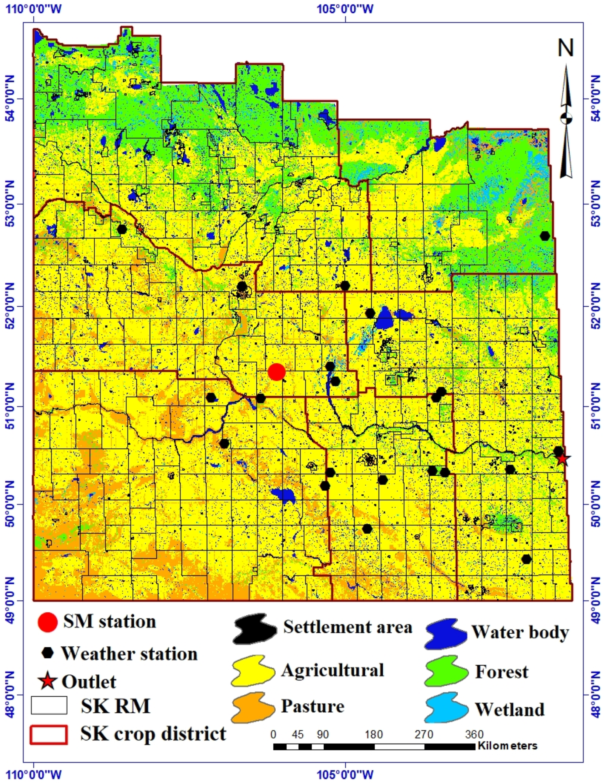
2.1. Study Area

This study was carried for the grain belt in Saskatchewan, which covers an area of 325,400 km². The agricultural land is divided into six crop districts in 296 rural municipalities (Figure 1) and thus, this study adopts a district-based approach, in contrast to the previous watershed-based investigations. Agricultural land use occupies about 62% of the total area. The primary crops cultivated in this region are wheat, canola, barley, flaxes, lentils, oats, peas, and soybeans. Since wheat and canola represent around 70% of the crop production, they were used for model calibration and validation. This region has a semi-arid to sub-humid continental climates, with very cold and dry winters and warm summers. Generally, snowmelt occurs in the spring season, resulting in higher streamflow during March and April. The average annual air temperature ranges from 8.0 °C to −3.5 °C and annual precipitation varies between 300 and 400 mm. The surface soil is classified into six major zones: dry brown, moist brown, dark brown, black, orthic gray, and dark gray.

2.2. Datasets

The daily weather data (precipitation, minimum temperature, maximum temperature, solar irradiation, wind speed, and relative humidity) over 1985 to 2020 were retrieved for 19 meteorological stations from Environment and Climate Change Canada (ECCC). Likewise, the daily streamflow discharge data for model calibration (1995–2004) and validation (2005–2010) were received from the hydrometric database (HYDAT) of Water Survey of Canada (WSC) for the Qu’Appelle River gauge near the Welby. The daily measured soil moisture data were retrieved for the Kenaston station to calibrate SWC in the model during the warm season (April 2015 to September 2020); the soil type information was derived from the Soil Landscapes of Canada (SLC ver. 3.2). The topographic data to delineate the watershed boundaries were extracted from a 30 m resolution Digital Elevation Model (Canadian GeoGratis). The 2015 land use database (30 m pixel) was compiled by Agriculture and Agri-Food Canada. Finally, the crop yield data according to RM were provided by the Saskatchewan Crop Insurance Corporation (SCIC).

In this study, we used 10 climate models of the North American-Coordinated Regional Climate Downscaling Experiment (NA-CORDEX) simulations (na-cordex.org). The daily climate model data were downloaded from the historical archives of the NA-CORDEX project. These data use a set of regional climate models (RCMs) to dynamically downscale various global climate models (GCMs) from the Coupled Model Inter-comparison Project Phase 5 (CMIP5) over the North American domain (Giorgi et al., 2009). Because the model output represents the raw data, ‘mbcn-Daymet’ was bias-corrected using Cannon’s MBCn algorithm versus Daymet gridded observational data for the daily data [36].

The analysis of crop yield used 10 simulations from the N-CORDEX ensemble at 0.22° or approximately 25 km spatial resolution, along with the Representative Concentration Pathway (RCP) 8.5 emission scenario. Climate change projections were derived from the NA-CORDEX RCMs from evaluating an array of climate variables for a historical baseline period (1975–2004) and three 30-year future periods: near (2010–2039), middle (2040–2069), and far (2070–2099).

2.3. SWAT-M Model

The SWAT model is a physically based hydrological formulation [14] that is used for a range of scales and environments, from small catchments to even continents [13]. This semi-distributed model breaks down a watershed into three parts, namely basin, sub-basin, and Hydrological Response Units (HRUs). The main parts of the model are climatic parameters, nutrient cycles, sediment transport, crop growth, and agricultural practices in different HRUs or sub-basins, in the form of daily, monthly, and yearly time points. Hydrologic simulations are based on the following water balance equation:

$$SS{W}_t=S{W}_o+{\sum }_{i=1}^t(R_{day}-Q_{surf}-E_a-W_{seep}-Q_{gw}{)}_i$$

(1)

In the above equation, $S{W}_t$ is final soil water content (mm), $S{W}_o$ is initial soil water content (mm), t is time (days), $R_{day}$ is cumulative precipitation (mm), $E_a$ is actual evapotranspiration (mm), $W_{seep}$ is percolation and bypass outflow from soil (mm), and $Q_{gw}$ is return flow on day $i$ (mm). Simulation of crop growth stages and crop yield are based on a simplified version of the Erosion Productivity Impact Calculator (EPIC) model [37]. The crop yield database has plant growth parameters for a wide range of land covers in the watershed at the HRU level.

The analysis of crop yield was adjusted for three plant growth parameters: radiation use efficiency (BIO_E); maximum potential leaf area index (BLAI); and harvest index (HVSTI), as defined below:

$${\gamma }_{reg}=1-\max (wstrs, tstrs, nstrs, pstrs)$$

(2)

In the above equation, ${\gamma }_{reg}$ is plant growth factor (0.0–1.0), whereas the daily stresses are $wstrs$ for water, $tstrs$ for temperature, $nstrs$ for nitrogen, and $pstrs$ for phosphorus. Only water and temperature stresses were considered, owing to a lack of data on nutrient and phosphorus cycling. For each crop of canola and wheat, three management practices of planting, fertilizing, and harvesting were applied based on the cropping calendar (day and month). Canola and wheat production was adjusted via observed harvests. The crop growth period was characterized by the total number of heat units (where each degree (°C) above the base temperature of the crop was taken as one heat unit), as per the following equation:

$$PHU={\sum }_{d=1}^{m}HU$$

(3)

where $PHU$ is total heat units for mature crops, and $HU$ is cumulative heat units on day d, with $d$ = 1 on sow date and $d$ = $m$ on crop maturity. Since harvest occurs at crop maturity, $m$ was counted from the planting date. Under optimal conditions (no growth stress), plant growth was modelled via daily biomass production that is governed by the amount of daily solar radiation intercepted by the leaf area of the plant, as per the following equation:

$$H_{phosyn}=0.5H_{day}·(1-\exp \left(-k_1·LAI\right))$$

(4)

where $H_{phosyn}$ is intercepted photo-synthetically active radiation on a given day ($\mathrm{M}\mathrm{J} {\mathrm{m}}^{-2})$, $H_{day}$ is incident total solar radiation ($\mathrm{M}\mathrm{J} {\mathrm{m}}^{-2})$, $0.5H_{day}$ is incident photo-synthetically active radiation ($\mathrm{M}\mathrm{J} {\mathrm{m}}^{-2})$, $k_1$ is light extinction coefficient, and LAI is leaf area index. Thereafter, the maximum rise in biomass on a given day was determined using the following equation [38]:

$$∆bio=RUE·H_{phosyn}$$

(5)

where $∆bio$ is potential increase in total plant biomass on a given day (kg/ha) and RUE is radiation-use efficiency of plants (${10}^{-1}\mathrm{g}/\mathrm{M}\mathrm{J}$). The total actual biomass accumulation over the growing season was obtained from the following equation:

$$bio={\sum }_{i=1}^d∆{bio}_i$$

(6)

where $bio$ is the total plant biomass on a given day ($\mathrm{k}\mathrm{g} {\mathrm{h}\mathrm{a}}^{-1}$).

One of the limitations of SWAT is that the aeration algorithm uses aeration stress (astrs) that, in turn, is based on the water content of the entire soil profile. This is appropriate when the roots are close to maturity but may not be adequate for shorter roots earlier in the growing season [29]. Therefore, the algorithm was modified for use in the water stress function. The water stress was predicted by comparing actual and potential transpiration using the following equation:

$$wstrs=1-\frac{E_{t,act}}{E_t}=1-\frac{w_{actualup}}{E_t}$$

(7)

where, for a given day, $wstrs$ is water stress, $E_t$ is maximum plant transpiration (mm H₂O), $E_{t,act}$ is actual transpiration (mm H₂O), and $w_{actualup}$ is total water uptake (mm H₂O). Both aeration stress and water stress have similar physiological patterns and require transformation based on expertise and experience [39]. These authors suggested the S-curve method to adjust yield to the original drought stress using the following equation:

$$wstrs=1-\frac{strsw}{strsw+\mathrm{e}\mathrm{x}\mathrm{p}(c1+c2\ast strsw)}$$

(8)

where $strsw$ is the ratio of actual to maximum transpiration.

Another limitation of the SWAT model concerns the simulation of streamflow in colder climates where runoff is mainly due to snowmelt in spring. Details on SWAT modifications such as functions and variables can be found in Zare et al. [20]. In this study, we combined the SWAT-M with the S-curve method to adjust yield to the original drought stress in the source code.

2.4. Model Calibration and Validation

The Calibration and Uncertainty Program (SWAT-CUP) and the Sequential Uncertainty Fitting (SUFI-2) programs were used for sensitivity analysis, as well as for calibration and uncertainty analysis of the modeling results. Multi-step calibration was applied including streamflow, soil moisture, and crop yield. First, the monthly data of the simulated and observed hydrographs for calibration (1995–2004) and validation (2005–2010) were compared. Two sensitivity rankings of ‘relative’ and ‘value’ were performed by the global sensitivity analysis technique in the SWAT-CUP. This was related to five algorithms and procedures in the SWAT: Sequential Uncertainty Fitting SUFI-2 Particle Swarm Optimization (POS), Generalized Likelihood Uncertainty Estimation (GLUE), Parameter Solution (ParaSol), and Mark Chain Monte Carlo (MCMC). Automated calibration and validation were carried out via SUFI-2 and uncertainty was obtained from input and output sources of uncertainty (rainfall, land use, soil type) as we inserted 35 parameters in the algorithm. The p-factor (measure of data in the 95% prediction) and the R-factor (ratio of average thickness of the p-factor to standard deviation in the measured data) were used to define the degree to which uncertainties are accounted for. After running this algorithm in the SWAT-CUP, we received 20 parameters, which means that the 20 most sensitive ones were given (including streamflow, groundwater, soil moisture, snow, and crop yield). The resulting sensitive parameters were calibrated against the observed runoff data from the outlet streamflow station. Based on the Qu’Appelle River basin in southern Saskatchewan [19], calibration and validation were extended to encompass the entire region after verifying the model’s performance.

Performance of the SWAT-M was evaluated by simultaneously using three statistical criteria for goodness-of-fit: the Nash–Sutcliffe efficiency (NSE) [40]; the percent bias (PBIAS) [41]; and the coefficient of correlation (r) [42], using the equations below, respectively:

$$NSE=\left[1-\frac{{{\sum }_{i=1}^n(Q_i^{obs}-{\overline{Q}}_i^{sim})}^2}{{\sum }_{i=1}^n{(Q_i^{obs}-Q_{mean}^{obs})}^2}\right]$$

(9)

$$PBIAS=\frac{{\sum }_{i=1}^n(Q_i^{obs}-Q_i^{sim})}{{\sum }_{i=1}^n{Q}_i^{obs}}\times 100$$

(10)

$$r=\frac{{\sum }_{i=1}^n\left(Q_i^{obs}-{\overline{Q}}_i^{obs}\right)·(Q_i^{sim}-{\overline{Q}}_i^{sim})}{\sqrt{\sum _{i=1}^n(Q_i^{obs}-{\overline{Q}}_i^{obs}{)}^2}·\sqrt{{\sum }_{i=1}^n(Q_i^{sim}-{\overline{Q}}_i^{sim}{)}^2}}$$

(11)

where, ${\overline{Q}}_i^{sim}$ and ${\overline{Q}}_i^{obs}$ are the mean monthly discharge values for simulation and observation, $Q_i^{obs}$ is observed discharge on day i, $Q_i^{sim}$ is simulated monthly discharge, n is number of months, and $Q_{mean}^{obs}$ is average observed monthly streamflow. After obtaining the best estimates of the parameters for streamflow calibration, SWC at the HRU level was derived in depth units (mm H₂O) at daily intervals. SWC was calibrated for the warm season (April to September) because measured data are generally missing for winter when the surface soil is frozen. The SWAT-M was calibrated for the annual yield of wheat and canola using average data to compare simulated and measured long-term crop yield (2005–2017) at the sub-basin level. To avoid analyzing 8618 individual HRUs, the average of multiple HRUs was used [12,33,35,43]. The size of the observation units (RM district) was not the same as the HRUs and therefore the average of multiple HRUs was applied.

2.5. Extreme Indices

To study the effects of extreme weather on crop yield, eight indices of precipitation and temperature were used (

Table 1. List of weather extreme indices for studying their impact on crop yield.

Indices	Description of Indices
Hot days	Number of days when $T_{max}>30 ℃$
Very wet days	Number of days with precipitation >$10 \mathrm{m}\mathrm{m}$
Freeze–thaw cycles	Freeze–thaw cycles occur when daily maximum temperature ($T_{max}$) > $0 ℃$ and daily minimum temperature ($T_{min}$) ≤ $-1 ℃$
Hot spell	No. of consecutive days when $T_{max}\ge 29 ℃$
Maximum 1-day precipitation	Amount of precipitation that falls on wettest day of the year (mm)
Longest Dry Spell	Maximum number of consecutive days when precipitation <$1 \mathrm{m}\mathrm{m}$
Longest Wet Spell	Maximum number of consecutive days when precipitation >$1 \mathrm{m}\mathrm{m}$
95th percentile precipitation (prcp95p)	No. of days during growing seasons when the precipitation >95th percentile of the base period 1975–2004

). The thresholds were defined by the CCI/CLIVAR/JCOMM Expert Team on Climate Change Detection and Indices (ETCCDI) [44]. The computation of these indices requires daily precipitation and temperature datasets. These indices assess three aspects of daily temperature and precipitation (minimum and maximum) regimes: the intensity (freeze–thaw cycles, maximum 1-day total precipitation), duration (hot spell, longest dry spell, longest wet spell), and frequency (hot days, very wet days, prcp95p) of weather events.

3. Results

3.1. Uncertainty, Sensitivity, and Calibration

Table 2. Initial parameter ranges for sensitivity and calibration analysis.

Rank	Parameters	Description	Initial Range	Calibrated Value
1	r_CN2.mgt	SCS curve number for moisture condition II	−0.2–0.2	0.17
2	v_ ALPHA_BF.gw	Baseflow alpha factor (days)	0.0–1.0	0.58
3	v_ GW_DELAY.gw	Groundwater delay (days)	−0.2–0.2	0.18
4	r_SOL_AWC.sol	Soil water available capacity	−0.1–1.0	0.37
5	v_GWQMN.gw	Threshold depth of water in shallow aquifer for return flow to occur (mm)	0–5000	4652
6	v_SMTMP.bsn	Snow melt base temperature (°C)	−5–5	2.61
7	v_SMFMN.bsn	Minimum snow melt rate per year (mm per °C d)	0–10	7.58
8	v_REVAP.gw	Groundwater “revap” coefficient	0.02–0.2	0.07
9	r__SOL_ALB(1).sol	Moist soil albedo in layer 1 of soil profile	−0.4–0.4	0.54
10	v_ESCO.hru	Soil evaporation compensation factor	0.0–1.0	0.45
11	r_SOL_Z.sol	Depth from the soil surface to layer bottom	−0.1–1.0	0.22
12	r_SOL_K.sol	Saturated hydraulic conductivity (mm/h)	−0.1–1.0	0.65
13	r_HVST I.dat(Canola)	Harvest index	0.4–0.5	0.47
14	r_WSYF.dat(Canola)	Lower limit of harvest index	0.3–0.35	0.33
15	r_BLAI.dat(Canola)	Maximum leaf area index	3–5	4.9
16	r_BIO_E.dat(Canola)	Radiation use efficiency	30–39	35.5
17	r_HVST I.dat(S.Wheat)	Harvest index	0.35–0.5	0.42
18	r_WSYF.dat(S.Wheat)	Lower limit of harvest index	0.3–0.4	0.36
19	r_BLAI.dat(S.Wheat)	Maximum leaf area index	3.5–7	6.4
20	r_BIO_E.dat(S.Wheat)	Radiation use efficiency	25–35	32

shows the results of sensitivity analyses, calibration and validation of SWAT-M streamflow, SWC, snowmelt, and crop yield over 16 years. The model was calibrated from 2000 to 2010 and validated from 2011 to 2016, along with a three-year warm-up time to mitigate the effect of initial unknown settings. Among the 35 input parameters, the 20 most sensitive ones are given (including streamflow, groundwater, soil moisture, snowmelt, and crop yield), based on the highest t-values and the highest significance (p-values → 0).

Figure 2 compares the observed and simulated streamflow data. NSE values were 0.66 during calibration and 0.79 during validation, thereby confirming satisfactory results at the monthly time point. Likewise, the corresponding PBIAS values were −5.3% and −7.7% for the two periods, suggesting good performance (PBIAS < ±10%) [7,45,46]. This indicates the model’s ability to properly simulate the stream discharge. Similarly, relatively high r-values (0.8 for both calibration and validation) result in closely matching observed and simulated streamflow data.

Figure 3 depicts a daily time series of soil moisture measurements from a sensor near Kenaston, SK, and the simulated SWC for the corresponding HRU (no. 918). The SWAT-M performed well for the warm season as indicated by the coefficient of correlation, PBIAS and NSE values of 0.7, 5.3 and 0.46, respectively. Likewise, the agreement of the daily time series confirmed the ability of the SWAT-M to predict SWC.

Figure 4 gives the results of calibration (2000–2009) and validation (2010–2019) for the annual yield of canola and wheat. The data for crop yield were collected from 2000 to 2019 at the RM level in bushels/ac unit. To compare with model output, these data were converted to kg/ha.

Table 3. Statistical analysis of the agreement between SWAT-M data and recorded annual crop yield.

Statistics	Calibration (2000–2009)		Validation (2010–2019)
	Canola	Spring Wheat	Canola	Spring Wheat
NSE	0.59	0.52	0.63	0.55
PBIAS (%)	−14.8	−14.4	−13.4	−9.6
r	0.62	0.66	0.78	0.72

gives the calibration and validation statistics for annual crop yield. The NSE values for canola and wheat were greater than 0.5 for both calibration and validation, indicating that the model performed satisfactorily for the annual time point [41]. The PBIAS values for the two crops also show acceptable performance (±10 < PBIAS < ±15%) [7,45,46]. Similarly, satisfactory values of r (±60 < PBIAS < ±75%) confirmed that the model was capable to satisfactorily predict annual wheat and canola yields during calibration.

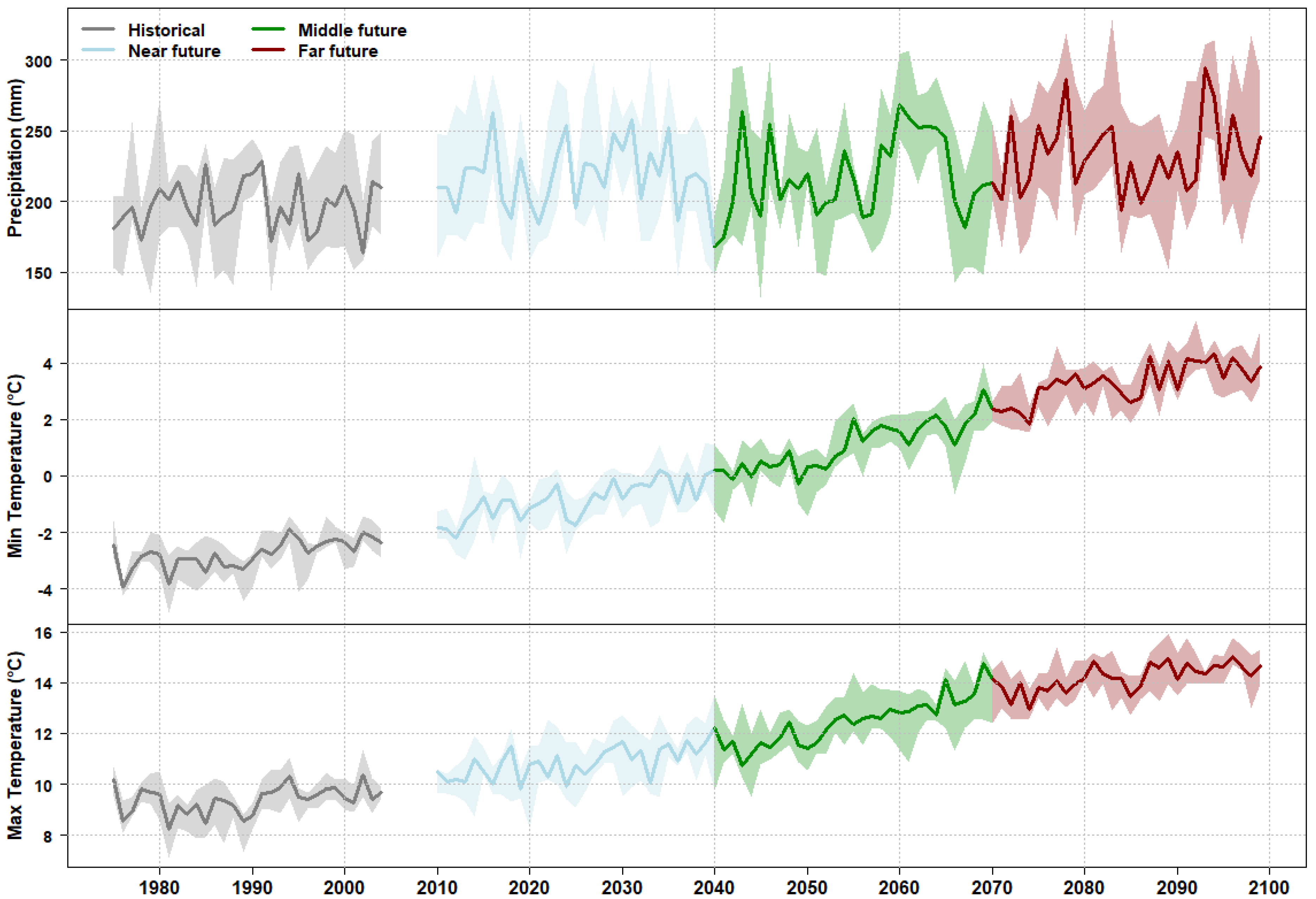
3.2. Projected Climate Changes

Figure 5 is a time series of the climate variables, showing the precipitation and maximum and minimum temperatures under historical conditions and future RCP8.5 forcing. The ensemble median precipitation was 197 mm in the baseline period, while it increased to 219, 218 and 233 mm during the near, middle, and far future periods, respectively. The ensemble median minimum temperature was −2.75 °C historically, rising to −0.89 °C in the near future, 1.1 °C in the middle future, and 3.3 °C in the far future. The median maximum temperature for the historical simulation was 9.4 °C, and increased to 10.8 °C, 12.4 °C, and 14.2 °C in the three periods, respectively.

The differences in projected seasonal precipitation and minimum and maximum temperatures relative to historical period are reported in

Table 4. The changes in projected average seasonal weather parameters relative to the historical baseline period.

Precipitation (mm)	2010–2039	2040–2069	2070–2099
JFM	1.82	8.82	16.82
AMJ	18.22	24.22	41.22
JAS	1.55	0.55	1.55
OND	4.9	3.9	4.9
Min Temperature (°C)	2010–2039	2040–2069	2070–2099
JFM	2.43	4.73	7.03
AMJ	2.07	3.17	4.52
JAS	1.24	3.04	5.54
OND	1.74	4.24	7.39
Max Temperature (°C)	2010–2039	2040–2069	2070–2099
JFM	1.73	3.29	5.09
AMJ	1.5	2.7	3.5
JAS	1	3	5.5
OND	1.36	3.2	5.38

. Precipitation, minimum temperature, and maximum temperature increased as expected in all seasons and periods; however, minimum temperature shows a greater increase than maximum temperature. The largest rise in temperature is projected to emerge during winter while the largest rise in precipitation is expected during spring.

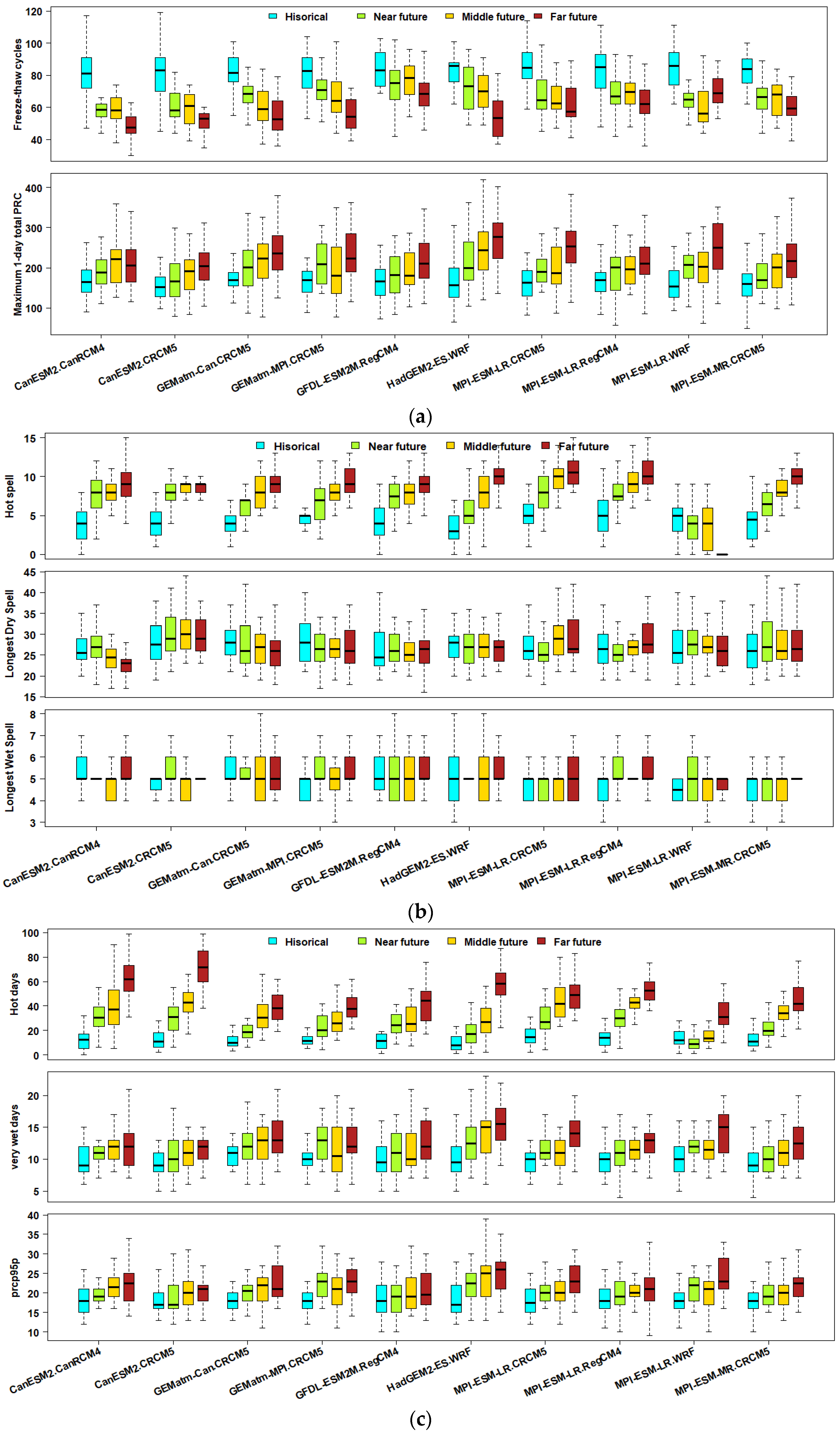
3.3. Projected Changes in Weather Indices

The results of extreme weather indices derived from 10 RCMs are presented as box plots in three categories of intensity, duration, and frequency (Figure 6a–c, respectively). They show that the number of freeze–thaw cycles per year decreases, while the results for the longest dry periods are mixed. The multi-model estimate projects a rise in the number of very wet days, maximum 1-day precipitation (PRC), duration of the longest wet periods, and 95th percentile precipitation index. Although there is no agreement among the RCM models for the temperature indices, the most variation in the projected relative changes was found in the precipitation indices. The results of the freeze–thaw cycles among all RCM models show that HadGEM2-ES.WRF in the historical period was the highest day (86 days), and CanESM2.CanRCM4 in the far future period indicated the lowest day (45 days). The medians of the maximum 1-day total precipitation show that the maximum value was 277mm in the HadGEM2-ES.WRF in the far future and the minimum value occurred at 152 mm in the CanESM2.CRCM5 for the historical period. For the hot spell indices, the higher increase was related to MPI-ESM-LR.CRCM5 with 11 days in the far future and the lower was in HadGEM2-ES.WRF with just 3 days in the historical. The longest dry spell values (30 days) of the future periods were generated by ESM2.CRCM5 for the middle future, while the longest wet spell was almost the same among all models and periods. The results of the indices for very wet days (95th percentile precipitation) show that HadGEM2-ES.WRF in the far future had the highest amount (16 and 26 days, respectively), and CanESM2.CRCM5 in the historical period indicated the lowest amount (9 and 17 days, respectively). The hot days data reveals that CanESM2.CRCM5 was the highest day (72 days) in the far future and that HadGEM2-ES.WRF was the lowest (8 days) in the historical period.

Figure 7 gives the temporal evolution of annual weather extreme indices under RCP8.5. These time series show an increasing trend for all indices, however, the temperature-related indices indicate a more pronounced upward trend compared to the rainfall-related indices. For instance, the hot days and hot spells indices are 11 and 4 days historically, while these values increase to 46 and 11 days in the late century, respectively.

The spatial variability of the historical and projected weather indices using the CMIP5 multi-model median is mapped in Figure 8. The projected variations in the longest wet spell and longest dry spell are small and fairly uniform across the region. The projected increase in the hot day frequency could exceed 10 to 70 days in the future, with the largest increase in southern parts of Saskatchewan. This pattern is quite similar for the hot spell index, albeit with less frequency overall. The smallest and highest spatial variability for very wet days was observed at Leader (in the west) and Hudson Bay (in the northeast), respectively. The spatial analysis also showed that there is a high variation in maximum 1-day total precipitation of around 300 mm in the northeast (far future map) and a smaller variation in the west of around 115 mm (historical map). On the contrary, the freeze–thaw cycle has the lowest frequency in the west, in the vicinity of Maple Creek (historical map), while this index is highest around Hudson Bay in the northeast (far future map).

3.4. Projected Change in Soil Water Content (SWC)

Figure 9 is a time series of the annual SWC under RCP8.5. The ensemble of 10 RCMs shows a decreasing trend towards the end of the century. The ensemble median SWC is 13.4% for the historical simulation, while it decreases to 11%, 9.5%, and 8.8% during the three future periods, respectively.

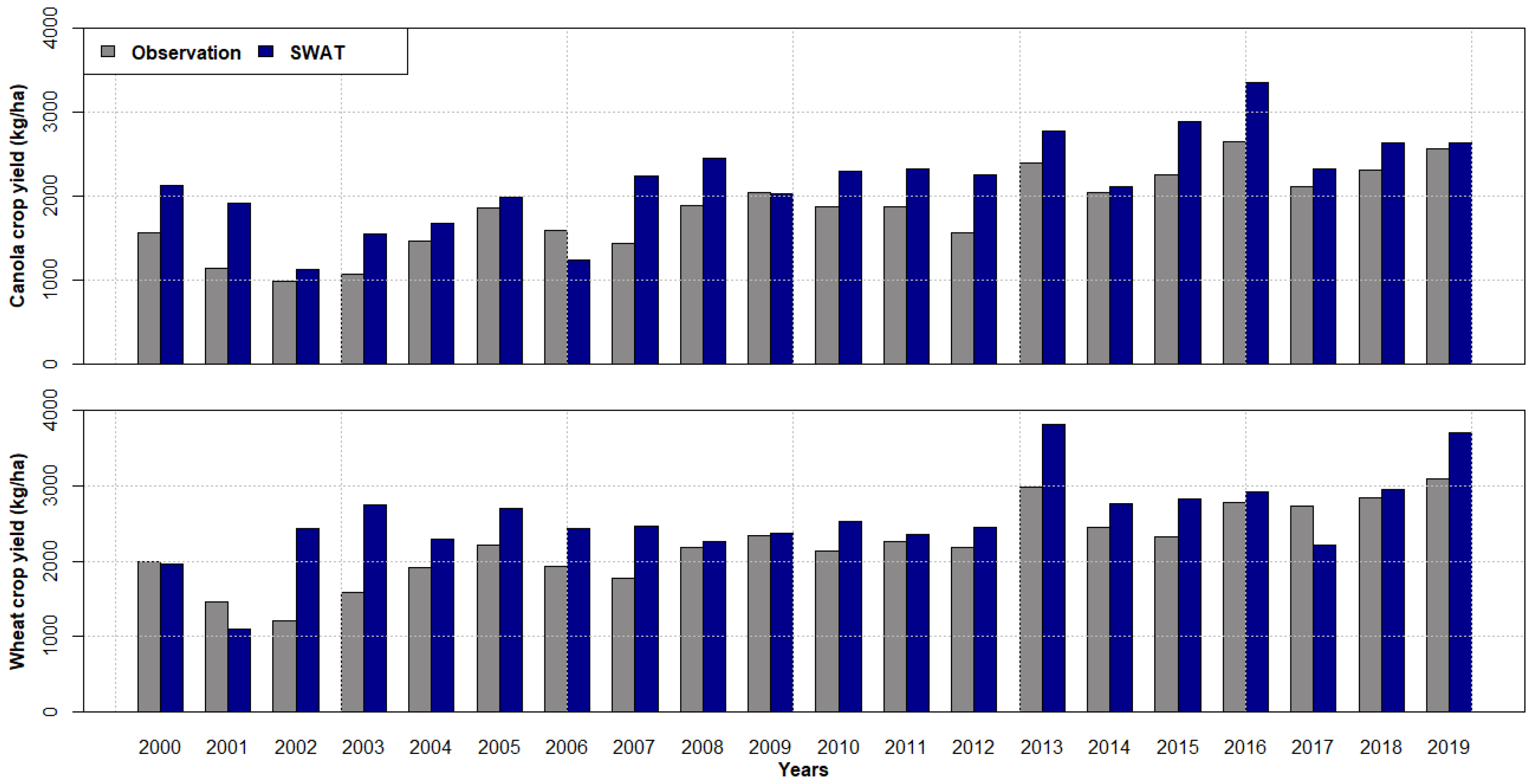
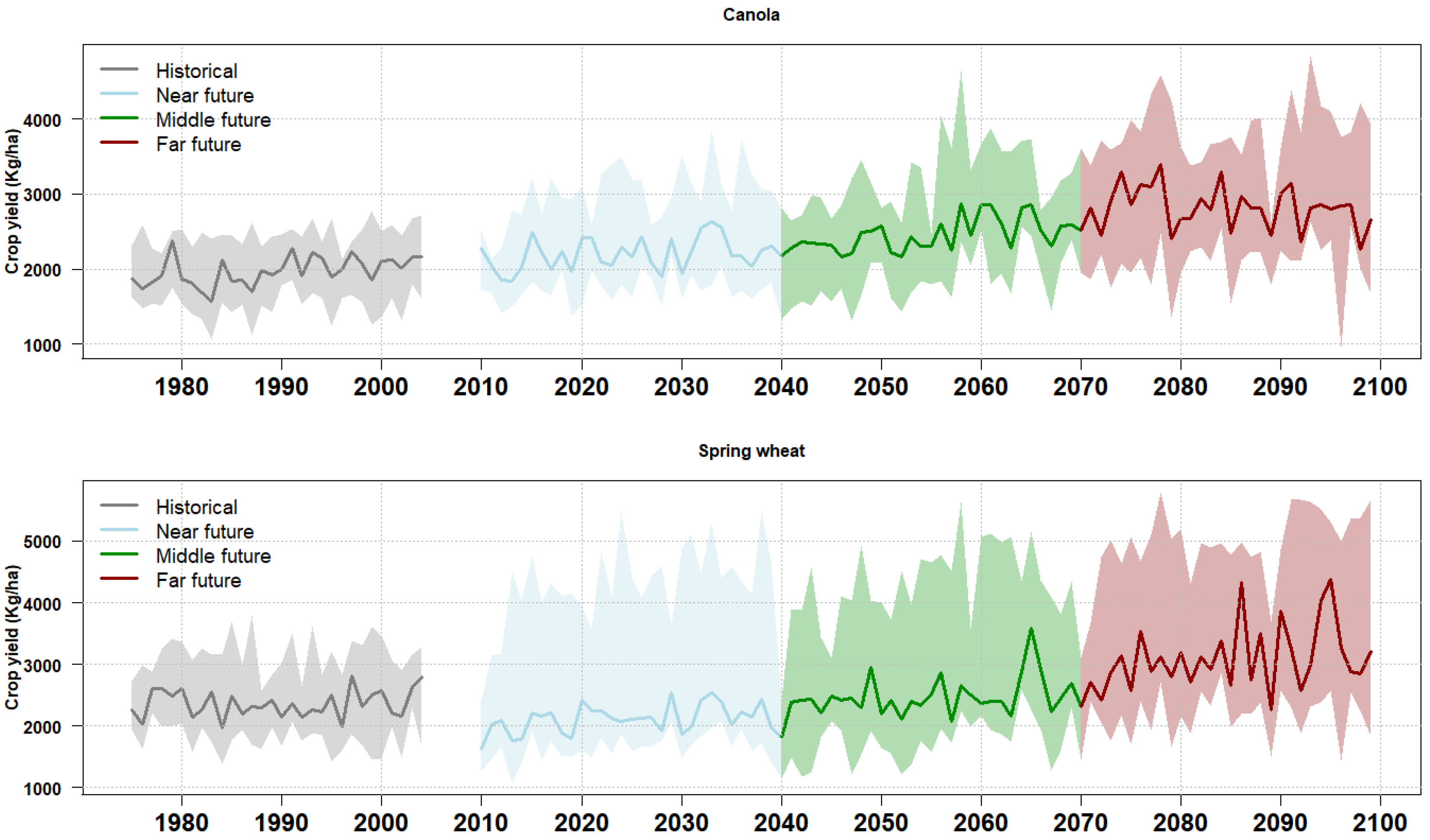
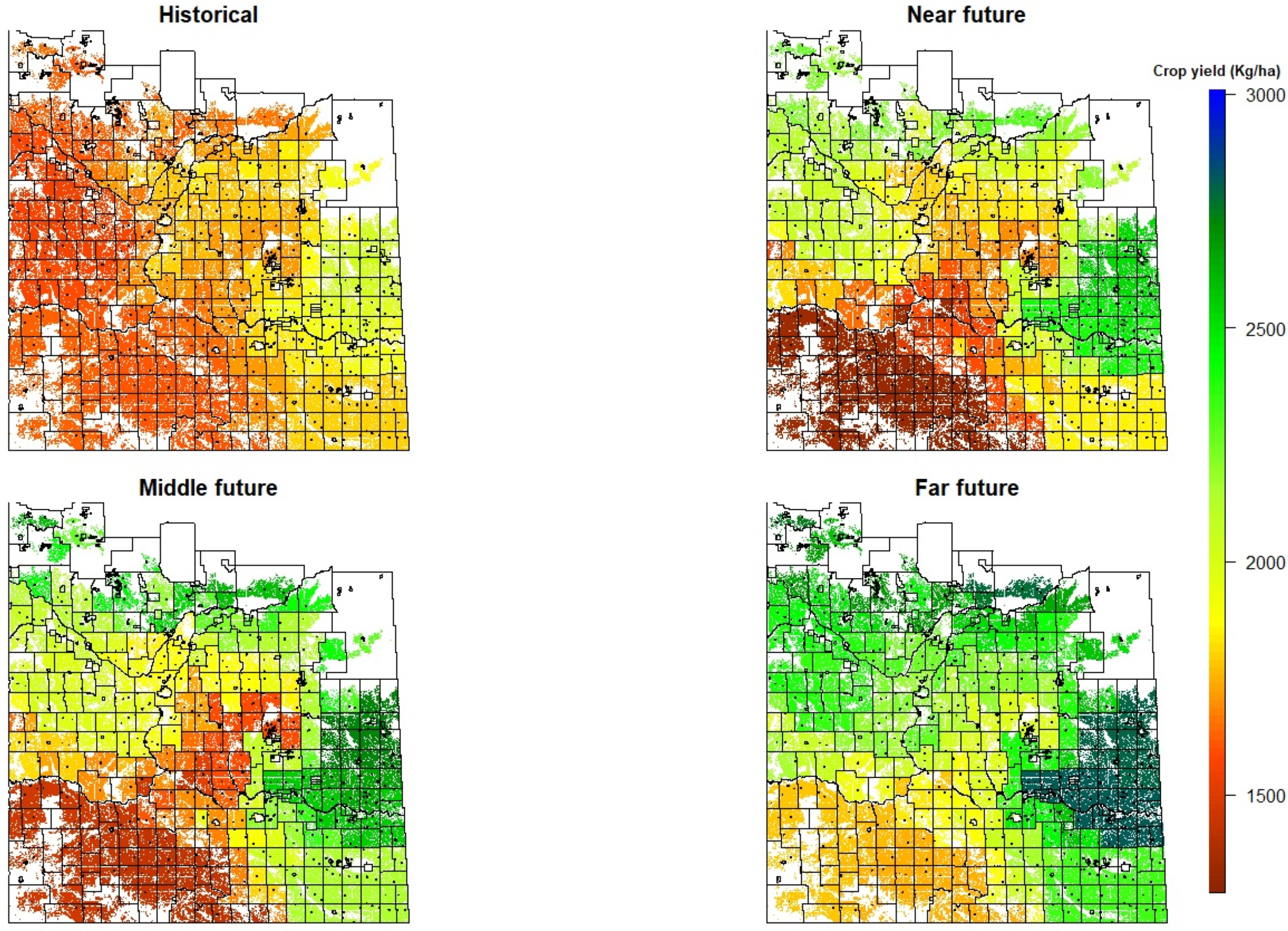
3.5. Impact of Climate Change on Crop Yield

Figure 10 gives the temporal evolution of annual crop yield under RCP8.5. The median values for an ensemble of 10 RCMs show an increasing trend towards the end of the current century. The historical median yields of canola and wheat were 1971 and 2360 Kg/ha, respectively. Canola increased by 2200, 2454, and 2771 Kg/ha during the near, middle, and far future, respectively. In contrast, wheat exhibits a different trend, with a decline of 2115 Kg/ha during the near future, followed by an increase to 2465 and 3047 Kg/ha in the middle and far future periods, respectively. Compared to the historical period, canola and wheat show an increase of 17 and 9.7% in the near future, 28.2 and 15.6% in the middle future, and 44.7 and 32% in the far future, respectively. However, under one RCM, MPI.ESM.LR.CRCM5, the yields decline by −6.86 to −0.48% for canola and −36.45 to −44.47 for spring wheat (Figure 11). Both canola and spring wheat yields increase across all other RCM models in the far future, except MPI.ESM.LR.CRCM5.

Figure 12 and Figure 13 are maps showing the spatial distribution of ensemble-median canola and wheat yield. Negative impacts on canola and wheat are projected for the southwest and central part of the region, particularly in the near and middle future, while positive effects could be expected in the northern and eastern parts of the area. However, under RCP8.5, no specific pattern of yield loss was identified in the far future compared to the baseline; yield is increased throughout southern Saskatchewan.

Figure 14 is a heat map of the Pearson correlation coefficients across all extreme weather indices and crop yield for the historical and projected periods. Canola yield has a high correlation with almost all weather indices except longest dry and wet spells, while spring wheat has a strong correlation with just hot spells. Several pairs of extreme indices had a strong positive or negative linear relationship; very wet days and maximum 1-day total precipitation show the strongest positive correlation.

4. Discussion

The most sensitive parameters were found to be soil moisture curve number (CN2) followed by Baseflow alpha factor (ALPHA_BF). Previous research [20,47,48] had similar findings for southern Saskatchewan. The first step of the calibration and validation processes revealed that the SWAT-M reproduced the hydrograph of measured monthly streamflow, including discharge peaks triggered by melting snow during April and May and low flows during summer and winter. Moreover, the SWAT-M simulated SWC with a good agreement to observed data in the investigated region by applying a combination of a physically based soil module with an energy budget for snowmelt during ROS events. Subsequently, the results were combined with the S-curve method to adjust yield to the original drought stress. In the context of southern Saskatchewan, the calibration and validation of the SWAT-M have demonstrated superior accuracy compared to previous research that utilized the original SWAT model [19] in the same region. The enhanced performance of the SWAT-M in this area highlights its effectiveness and potential for more precise and reliable results. These findings suggest that the SWAT-M could be an invaluable means for future studies and water resource management in the prairie region.

Similarly, the predicted crop yields generally agree with measured data, however, with lesser performance compared with streamflow and SWC, along with overestimation in some years. For instance, the model overestimated canola yield by around 800 kg/h in 2007; a similar situation happened for wheat, where the estimates of yield were 1227 kg/ha higher than observed in 2002. Abbaspour et al. [49], Hu et al. [50], Nair et al. [51], and Srinivasan et al. [52] also showed that the SWAT model simulates crop yield well. However, they mentioned the challenges associated with limited input data at the farm scale. Sinnathamby et al. [12] reported an overestimation of corn yield by the SWAT. It is difficult for SWAT simulations to accurately reflect the impact of heat stress, as the SWAT is primarily influenced by the daily mean temperature. Consequently, the simulation tends to overestimate yield under hot dry conditions, such as in the 2002 growing season.

Eight weather extreme indices were analyzed in terms of their temporal and spatial variability and their correlation with crop yield in southern Saskatchewan. The multi-model ensemble showed an increasing radiative forcing over time of temperature and precipitation indices, similar to the findings of previous studies using climate models [53,54,55,56]. The RCMs project warmer and wetter conditions relative to a historical baseline. The greatest warming is found over the south and southwest of Saskatchewan and the largest increase in precipitation indices is in the north and northeast. Warmer temperatures will be beneficial for agriculture because they will be accompanied by longer frost-free seasons and more growing degree days [57]. The results for canola and wheat indicate an increase of 17 and 9.7% in the near future, 28.2 and 15.6% in the middle future, and 44.7 and 32% in the far future, respectively, under rain-fed conditions. These results are comparable to modeling crop yield at specific sites in the region. Smith et al. [58] estimated an increase of 37% for spring wheat using the DNDC model in the Canadian Prairies for 2050. Qian et al. [5] found an increase of 26 to 37% during 2041–2070 compared with the baseline period of 1971–2000 using the DSSAT model. Using CanRCM4 climate data and the DSSAT model, He et al. (2018) also determined that spring wheat yield will increase by 15%. Our research, extending across southern Saskatchewan, indicated that despite an overall increase in median annual wheat and canola yield, the crop yield in the extreme south and southwest regions shows a significant decrease, reaching around 1000 $\mathrm{k}\mathrm{g} {\mathrm{h}\mathrm{a}}^{-1}$ for the near and middle future.

Excessively high temperatures can harm crops even if the region receives adequate rainfall. Water stress in the middle future results from a large increase in temperature but only a minor increase in precipitation during the growing season. Extreme temperature indices, like hot days, have a strong correlation with crop yield, and their adverse impact on rain-fed agricultural production is difficult to mitigate [59,60]. Qian et al. [7] suggested that simulated wheat production may benefit from an elevated atmospheric CO₂ concentration as water use is accompanied by increased precipitation in the prairie regions. Despite the declining trend of soil moisture towards the end of the current century, there is an overall upward trend in crop yield. It appears that the simulation of crop yield is significantly more affected by weather conditions than by soil moisture content. The determination of planting dates is therefore based on heat units in the SWAT-M, focusing solely on temperature rather than soil moisture levels. Among the climate models, MPI-ESM-LR.CRCM5 gives the driest conditions and thus shows the most negative changes, while HadGEM2-ES.WRF gives the wettest climate forcing and thus produces the most positive change in canola and wheat yield.

Generally, the SWAT-M has some limitations for simulating crop yield under the effect of climate change. According to Ficklin et al. [61], the increase in atmospheric CO₂ concentrations may directly impact the hydrological cycle. Some plants may experience stomatal closure due to high CO₂ concentrations, leading to reduced transpiration rates at the leaf level, as noted in research works by Field et al. [62], Medlyn et al. [63], Saxe et al. [64], Wand et al. [65], Leakey et al. [66], Sreeharsha et al. [67], and Xu et al. [68]. The model assumes a linear reduction in stomatal conductance over a wide range of CO₂ concentrations from 330 ppm to 660 ppm [69]. Still, the average atmospheric CO₂ concentration predicted under the RCP8.5 scenario for 2060–2099 (far future) is 958 ppm, which is more than 660 ppm as simulated by the SWAT. This means that caution is necessary when interpreting the CO₂ effect on crop yields and further studies need to be conducted at higher atmospheric CO₂ concentrations [35].

The fertile grassland soils of the northern Great Plains are ideal for cultivating cereal, oil seed, and pulse crops; however, the dry cold climate is amongst the least favorable on Earth where commercial agriculture is practiced. A viable agricultural industry exists in western Canada because agricultural produces have adapted farming practices and adopted technology to overcome the limitations imposed by short growing seasons and the sub-humid climate. Notable examples among these adaptations are drought-resistant and early-maturing crops, irrigation, GPS-guided precision agriculture, crop rotations, and transitions to minimal soil tillage. Further adaptions will be required to achieve the higher crop yields projected by our study and to prevent crop losses in years with insufficient soil moisture. Our simulation of crop yield in the SWAT model was based on current land use and management practices. Although the SWAT-M cannot replicate random events like severe weather incidents, which can lead to differences between the predicted and actual annual yields during calibration and validation, it is able to predict the impact of long-term changes in average conditions.

5. Conclusions

We used an improved SWAT model for simulating the possible impacts of climate change on the yield of two important crops (wheat and canola) in southern Saskatchewan. In this research, we integrated the SWAT-M model with the S-curve method to modify crop yield within the source code, to adjust yield to the original drought stress. The results showed that streamflow, SWC, and crop yield can be successfully modeled using the calibrated SWAT-M. However, crop yield calibration results show less performance compared with streamflow and SWC along with overestimation, so the model did not predict yield quite well in some years. The simulation of eight extreme indices using 10 RCMs revealed a significant increase in temperature indices in all crop districts and a decreasing trend for the number of freeze–thaw cycles. Moreover, almost all climate models predicted an increasing trend for precipitation indices compared to historical values. The regional spatial pattern of climate extremes showed that the southern part of the area becomes much drier and warmer whereas the northern part becomes wetter. Multi-model median canola and wheat yields were predicted to increase by the end of the current century. It appears that future global warming resulting in increased precipitation will be beneficial to crop yield, particularly in the far future. However, crop models that solely rely on changes in average conditions fail to account for the potential offsetting effects of weather extremes, thereby leading to overestimations of crop yields in the long run. The spatial pattern of the crop yield suggests a significant decrease in production in the south and southwest regions, with the drop in yield reaching to 1000 $\mathrm{k}\mathrm{g} {\mathrm{h}\mathrm{a}}^{-1}$ for the near and middle future. The findings of this research can offer farmers and policymakers a scientific foundation for devising strategies to deal with the impacts of climate change. These measures can be implemented to attain maximum and high-quality yields of canola and spring wheat, ultimately ensuring food security.

References

1. Statistics Canada. Total Area of Farms and Use of Farm Land, Historical Data. 2016. Available online: https://www150.statcan.gc.ca/t1/tbl1/en/tv.action?pid=3210015301&pickMembers%5B0%5D=1.9&pickMebers%5B1%5D=3.2 (accessed on 15 January 2023).
2. Government of Saskatchewan. Saskatchewan Agricultural Exports. 2015; 25p. Available online: http://publications.gov.sk.ca/documents/20/83881-Saskatchewan%20Agriculture%20Exports%202015.pdf (accessed on 23 March 2015).
3. Kerr, S.A.; Andreichuk, Y.; Sauchyn, D.J. Re-Evaluating the Climate Factor in Agricultural Land Assessment in a Changing Climate—Saskatchewan, Canada. Land 2019, 8, 49. [Google Scholar] [CrossRef]
4. Bradshaw, B.; Dolan, H.; Smit, B. Farm-Level Adaptation to Climatic Variability and Change: Crop Diversification in the Canadian Prairies. Clim. Change 2004, 67, 119–141. [Google Scholar] [CrossRef]
5. Qian, B.; De Jong, R.; Huffman, T.; Wang, H.; Yang, J. Projecting yield changes of spring wheat under future climate scenarios on the Canadian Prairies. Theor. Appl. Climatol. 2016, 123, 651–669. [Google Scholar] [CrossRef]
6. He, W.; Yang, J.Y.; Qian, B.; Drury, C.F.; Hoogenboom, G.; He, P.; Lapen, D.; Zhou, W. Climate change impacts on crop yield, soil water balance and nitrate leaching in the semiarid and humid regions of Canada. PLoS ONE 2018, 13, e0207370. [Google Scholar] [CrossRef]
7. Qian, B.; Zhang, X.; Smith, W.; Grant, B.; Jing, Q.; Cannon, A.J.; Neilsen, D.; McConkey, B.; Li, G.; Bonsal, B. Climate change impacts on Canadian yields of spring wheat, canola and maize for global warming levels of 1.5 C, 2.0 C, 2.5 C and 3.0 C. Environ. Res. Lett. 2019, 14, 074005. [Google Scholar] [CrossRef]
8. Qian, B.; Jing, Q.; Smith, W.; Grant, B.; Cannon, A.J.; Zhang, X. Quantifying the uncertainty introduced by internal climate variability in projections of Canadian crop production. Environ. Res. Lett. 2020, 15, 074032. [Google Scholar] [CrossRef]
9. Field, C.B.; Barros, V.; Stocker, T.F.; Qin, D.; Dokken, D.J.; Ebi, K.L.; Mastrandrea, M.D.; Mach, K.J.; Plattner, G.-K.; Allen, S.K.; et al. (Eds.) Managing the Risks of Extreme Events and Disasters to Advance Climate Change Adaptation. A Special Report of Working Groups I and II of the Intergovernmental Panel on Climate Change; Cambridge University Press: Cambridge, UK; New York, NY, USA, 2012. [Google Scholar]
10. Moss, R.H.; Edmonds, J.A.; Hibbard, K.A.; Manning, M.R.; Rose, S.K.; Van Vuuren, D.P.; Carter, T.R.; Emori, S.; Kainuma, M.; Kram, T. The next generation of scenarios for climate change research and assessment. Nature 2010, 463, 747–756. [Google Scholar] [CrossRef]
11. Van Vuuren, D.P.; Edmonds, J.; Kainuma, M.; Riahi, K.; Thomson, A.; Hibbard, K. The representative concentration pathways: An overview. Clim. Change 2011, 109, 5–31. [Google Scholar] [CrossRef]
12. Sinnathamby, S.; Douglas-Mankin, K.R.; Craige, C. Field-scale calibration of crop-yield parameters in the Soil and Water Assessment Tool (SWAT). Agric. Water Manag. 2017, 180, 61–69. [Google Scholar] [CrossRef]
13. Arnold, J.G.; Moriasi, D.N.; Gassman, P.W.; Abbaspour, K.C.; White, M.J.; Srinivasan, R.; Santhi, C.; Harmel, R.D.; Van Griensven, A.; Van Liew, M.W.; et al. SWAT: Model use, calibration, and validation. Trans. ASABE 2012, 55, 1491–1508. [Google Scholar] [CrossRef]
14. Arnold, J.G.; Srinivasan, R.; Muttiah, R.S.; Williams, J.R. Large Area Hydrologic Modeling and Assessment Part I: Model Development. J. Am. Water Resour. Assoc. 1998, 34, 73–89. [Google Scholar] [CrossRef]
15. Zhang, J.; Li, S.Y.; Dong, R.Z.; Jiang, C.S.; Ni, M.F. Influences of land use metrics at multi-spatial scales on seasonal water quality: A case study of river systems in the Three Gorges Reservoir Area. China J. Clean. Prod. 2019, 206, 76–85. [Google Scholar] [CrossRef]
16. Liu, W.; Park, S.; Bailey, R.T.; Molina-Navarro, E.; Andersen, H.E.; Thodsen, H.; Nielsen, A.; Jeppesen, E.; Jensen, J.S.; Jensen, J.B.; et al. Comparing SWAT with SWAT-MODFLOW hydrological simulations when assessing the impacts of groundwater abstractions for irrigation and drinking water. Hydrol. Earth Syst. Sci. Discuss. 2019, 232, 1–51. [Google Scholar]
17. Meaurio, M.; Zabaleta, A.; Uriarte, J.A.; Srinivasan, R.; Antigüedad, I. Evaluation of SWAT models performance to simulate streamflow spatial origin. The case of a small forested watershed. J. Hydrol. 2015, 525, 326–334. [Google Scholar] [CrossRef]
18. Rahman, K.U.; Pham, Q.B.; Jadoon, K.Z.; Shahid, M.; Kushwaha, D.P.; Duan, Z.; Mohammadi, B.; Khedher, K.M.; Anh, D.T. Comparison of Machine Learning and Process-Based SWAT Model in Simulating Streamflow in the Upper Indus Basin. Appl. Water Sci. 2022, 12, 178. [Google Scholar] [CrossRef]
19. Zare, M.; Azam, S.; Sauchyn, D. Evaluation of Soil Water Content Using SWAT for Southern Saskatchewan, Canada. Water 2022, 14, 249. [Google Scholar] [CrossRef]
20. Zare, M.; Azam, S.; Sauchyn, D. A Modified SWAT Model to Simulate Soil Water Content and Soil Temperature in Cold Regions: A Case Study of the South Saskatchewan River Basin in Canada. Sustainability 2022, 14, 10804. [Google Scholar] [CrossRef]
21. Rajib, A.; Merwade, V.; Kim, I.L.; Zhao, L.; Song, C.; Zhe, S. SWATShare—A web platform for collaborative research and education through online sharing, simulation and visualization of SWAT models. Environ. Model. Softw. 2016, 75, 498–512. [Google Scholar] [CrossRef]
22. Havrylenko, S.B.; Bodoque, J.M.; Srinivasan, R.; Zucarelli, G.V.; Mercuri, P. Assessment of the soil water content in the Pampas region using SWAT. Catena 2016, 137, 298–309. [Google Scholar] [CrossRef]
23. Uniyal, B.; Dietrich, J.; Vasilakos, C.; Tzoraki, O. Evaluation of SWAT simulated soil moisture at catchment scale by field measurements and Landsat derived indices. Agric. Water Manag. 2017, 193, 55–70. [Google Scholar] [CrossRef]
24. Qi, J.; Zhang, X.; Wang, Q. Improving hydrological simulation in the Upper Mississippi River Basin through enhanced freeze-thaw cycle representation. J. Hydrol. 2019, 571, 605–618. [Google Scholar] [CrossRef]
25. Vigiak, O.; Malagó, A.; Bouraoui, F.; Vanmaercke, M.; Obreja, F.; Poesen, J.; Habersack, H.; Fehér, J.; Grošelj, S. Modelling sediment fluxes in the Danube River Basin with SWAT. Sci. Total Environ. 2017, 599–600, 992–1012. [Google Scholar] [CrossRef] [PubMed]
26. Yesuf, H.M.; Assen, M.; Alamirew, T.; Melesse, A.M. Modeling of sediment yield in Maybar gauged watershed using SWAT, northeast Ethiopia. Catena 2015, 127, 191–205. [Google Scholar] [CrossRef]
27. Malagó, A.; Bouraoui, F.; Vigiak, O.; Grizzetti, B.; Pastori, M. Modelling water and nutrient fluxes in the Danube River Basin with SWAT. Sci. Total Environ. 2017, 603–604, 196–218. [Google Scholar] [CrossRef] [PubMed]
28. Xie, X.; Cui, Y. Development and Test of SWAT for Modeling Hydrological Processes in Irrigation Districts with Paddy Rice. J. Hydrol. 2011, 396, 61–71. [Google Scholar] [CrossRef]
29. Wang, R.; Bowling, L.C.; Cherkauer, K.A. Estimation of the effects of climate variability on crop yield in the Midwest USA. Agric. For. Meteorol. 2016, 216, 141–156. [Google Scholar] [CrossRef]
30. Mittelstet, A.R.; Storm, D.E.; Stoecker, A.L. Using SWAT to simulate crop yields and salinity levels in the North Fork River Basin, USA. Int. J. Agric. Biol. Eng. 2015, 8, 110–124. [Google Scholar]
31. Chen, Y.; Marek, G.W.; Marek, T.H.; Porter, D.O.; Brauer, D.K.; Srinivasan, R. Simulating the effects of agricultural production practices on water conservation and crop yields using an improved SWAT model in the Texas High Plains, USA. Agric. Water Manag. 2021, 244, 106574. [Google Scholar] [CrossRef]
32. Bauwe, A.; Kahle, P.; Lennartz, B. Evaluating the SWAT model to predict streamflow, nitrate loadings and crop yields in a small agricultural catchment. Adv. Geosci. 2019, 48, 1–9. [Google Scholar] [CrossRef]
33. Sun, C.; Ren, L. Assessing crop yield and crop water productivity and optimizing irrigation scheduling of winter wheat and summer maize in the Haihe plain using SWAT model. Hydrol. Process. 2014, 28, 2478–2498. [Google Scholar] [CrossRef]
34. Musyoka, F.K.; Strauss, P.; Zhao, G.; Srinivasan, R.; Klik, A. Multi-step calibration approach for SWAT model using soil moisture and crop yields in a small agricultural catchment. Water 2021, 13, 2238. [Google Scholar] [CrossRef]
35. Kang, X.; Qi, J.; Li, S.; Meng, F.-R. A watershed-scale assessment of climate change impacts on crop yields in Atlantic Canada. Agric. Water Manag. 2022, 269, 107680. [Google Scholar] [CrossRef]
36. Mearns, L.; McGinnis, S.; Korytina, D.; Arritt, R. The NA-CORDEX Dataset; Version 1.0.; NCAR Climate Data Gateway: Boulder, CO, USA, 2017; Available online: https://na-cordex.org/ (accessed on 16 May 2017).
37. Williams, J.R. The erosion-productivity impact calculator (EPIC) model: A case history. Philos. Trans. Roy. Soc. B 1990, 329, 421–428. [Google Scholar]
38. Monteith, J.L. Climate and efficiency of crop production in Britain. Philos. Trans. Roy. Soc. B 1977, 281, 277–284. [Google Scholar]
39. Kozak, J.A.; Ma, L.; Ahuja, L.R.; Flerchinger, G.; Nielsen, D.C. Evaluating various water stress calculations in RZWQM and RZ-SHAW for corn and soybean production. Agron. J. 2006, 98, 1146–1155. [Google Scholar] [CrossRef]
40. Nash, J.E.; Sutcliffe, J.V. River flow forecasting through conceptual models: Part I—A discussion of principles. J. Hydrol. 1970, 10, 282–290. [Google Scholar] [CrossRef]
41. Moriasi, D.N.; Arnold, J.G.; Van Liew, M.W.; Binger, R.L.; Harmel, R.D.; Veith, T. Model evaluation guidelines for systematic quantification of accuracy in watershed simulations. Trans. ASABE 2007, 50, 885–900. [Google Scholar] [CrossRef]
42. Legates, D.R.; McCabe, G.J. Evaluating the use of “goodness-of-fit” measures in hydrologic and hydroclimatic model vali-dation. Water Resour. Res. 1999, 35, 233–241. [Google Scholar] [CrossRef]
43. Shahvari, N.; Khalilian, S.; Mosavi, S.H.; Mortazavi, S.A. Assessing climate change impacts on water resources and crop yield: A case study of Varamin plain basin, Iran. Environ. Monit. Assess. 2019, 191, 134. [Google Scholar] [CrossRef]
44. Karl, T.R.; Nicholls, N.; Ghazi, A. Clivar. GCOS/WMO workshop on indices and indicators for climate extremes workshop summary. In Weather and Climate Extremes; Springer: Dordrecht, The Netherlands, 1999; pp. 3–7. [Google Scholar]
45. Pomeroy, J.; Fang, X.; Williams, B. Impacts of Climate Change on Saskatchewan’s Water Resources; Centre for Hydrology, University of Saskatchewan: Saskatoon, SK, Canada, 2009. [Google Scholar]
46. Abbaspour, K.C.; Yang, J.; Maximov, I.; Siber, R.; Bogner, K.; Mieleitner, J.; Zobrist, J.; Srinivasan, R. Modelling hydrology and water quality in the pre-alpine/alpine Thur watershed using SWAT. J. Hydrol. 2007, 333, 413–430. [Google Scholar] [CrossRef]
47. Perez-Valdivia, C.; Cade, B.; McMartin, D. Hydrological modeling of the pipestone creek watershed using the Soil Water Assessment Tool (SWAT): Assessing impacts of wetland drainage on hydrology. J. Hydrol. 2017, 14, 109–129. [Google Scholar] [CrossRef]
48. Mekonnen, B.; Mazurek, K.; Putz, G. Incorporating landscape depression heterogeneity into the Soil and Water Assessment Tool (SWAT) using a probability distribution. Hydrol. Process. 2016, 30, 2373–2389. [Google Scholar] [CrossRef]
49. Abbaspour, K.C.; Rouholahnejad, E.; Vaghefi, S.; Srinivasan, R.; Yang, H.; Kløve, B. A continental-scale hydrology and water quality model for Europe: Calibration and uncertainty of a high-resolution large-scale SWAT model. J. Hydrol. 2015, 524, 733–752. [Google Scholar] [CrossRef]
50. Hu, X.; McIsaac, G.F.; David, M.B.; Louwers, C.A.L. Modeling Riverine Nitrate Export from an East-Central Illinois Watershed Using SWAT. J. Environ. Qual. 2007, 36, 996–1005. [Google Scholar] [CrossRef] [PubMed]
51. Nair, S.S.; King, K.; Witter, J.D.; Sohngen, B.L.; Fausey, N.R. Importance of Crop Yield in Calibrating Watershed Water Quality Simulation Tools 1. J. Am. Water Resour. Assoc. 2011, 47, 1285–1297. [Google Scholar] [CrossRef]
52. Srinivasan, R.; Zhang, X.; Arnold, J. SWAT ungauged: Hydrological budget and crop yield predictions in the upper Mississippi River basin. Trans. ASABE 2010, 53, 1533–1546. [Google Scholar] [CrossRef]
53. Kiktev, D.; Sexton, D.; Alexander, L.; Folland, C. Comparison of Modeled and Observed Trends in Indices of Daily Climate Extremes. J. Clim. 2003, 16, 3560–3571. [Google Scholar] [CrossRef]
54. Min, S.-K.; Zhang, X.; Zwiers, F.W.; Hegerl, G.C. Human contribution to more-intense precipitation extremes. Nature 2011, 470, 378–381. [Google Scholar] [CrossRef]
55. Sillmann, J.; Kharin, V.V.; Zhang, X.; Zwiers, F.W.; Bronaugh, D. Climate extremes indices in the CMIP5 multimodel ensemble: Part 1. Model evaluation in the present climate. J. Geophys. Res. Atmos. 2013, 118, 1716–1733. [Google Scholar] [CrossRef]
56. Sillmann, J.; Kharin, V.V.; Zwiers, F.W.; Zhang, X.; Bronaugh, D. Climate extremes indices in the CMIP5 multimodel ensemble: Part 2. Future climate projections. J. Geophys. Res. Atmos. 2013, 118, 2473–2493. [Google Scholar] [CrossRef]
57. Vincent, L.A.; Wang, X.L.; Milewska, E.J.; Wan, H.; Yang, F.; Swail, V. A second generation of homogenized Canadian monthly surface air temperature for climate trend analysis. J. Geophys. Res. Atmos. 2012, 117. [Google Scholar] [CrossRef]
58. Smith, W.N.; Grant, B.B.; Desjardins, R.L.; Kroebel, R.; Li, C.; Qian, B.; Worth, D.E.; McConkey, B.G.; Drury, C.F. Assessing the effects of climate change on crop production and GHG emissions in Canada. Agric. Ecosyst. Environ. 2013, 179, 139–150. [Google Scholar] [CrossRef]
59. Thomson, A.M.R.A.; Brown, N.J.; Rosenberg, N.J.; Lazaurralde, R.C.; Benson, V. Climate change impacts for the conterminous USA: An integrated assessment Part 3. Dry land production of grain and forage Crops. Clim. Change 2005, 69, 43–65. [Google Scholar] [CrossRef]
60. Ko, J.; Ahuja, L.R.; Saseendran, S.; Green, T.R.; Ma, L.; Nielsen, D.C.; Walthall, C.L. Climate change impacts on dryland cropping systems in the Central Great Plains, USA. Clim. Change 2012, 111, 445–472. [Google Scholar] [CrossRef]
61. Ficklin, D.L.; Robeson, S.M.; Knouft, J.H. Impacts of recent climate change on trends in baseflow and stormflow in United States watersheds. Geophys. Res. Lett. 2016, 43, 5079–5088. [Google Scholar] [CrossRef]
62. Field, C.B.; Jackson, R.B.; Mooney, H.A. Stomatal responses to increased CO2: Implications from the plant to the global scale. Plant Cell Environ. 1995, 18, 1214–1225. [Google Scholar] [CrossRef]
63. Medlyn, B.E.; Barton, C.V.M.; Broadmeadow, M.S.J.; Ceulemans, R.; De Angelis, P.; Forstreuter, M.; Freeman, M.; Jackson, S.B.; Kellomäki, S.; Laitat, E.; et al. Stomatal conductance of forest species after long-term exposure to elevated CO2 concentration: A synthesis. New Phytol. 2001, 149, 247–264. [Google Scholar] [CrossRef]
64. Saxe, H.; Ellsworth, D.S.; Heath, J. Tree and forest functioning in an enriched CO2 atmosphere. New Phytol. 1998, 139, 395–436. [Google Scholar] [CrossRef]
65. Wand, S.J.E.; Midgley, G.F.; Jones, M.H.; Curtis, P.S. Responses of wild C4 and C3 grass (Poaceae) species to elevated atmospheric CO2 concentration: A meta-analytic test of current theories and perceptions. Glob. Chang. Biol. 1999, 5, 723–741. [Google Scholar] [CrossRef]
66. Leakey, A.D.; Ainsworth, E.A.; Bernacchi, C.J.; Rogers, A.; Long, S.P.; Ort, D.R. Elevated CO2 effects on plant carbon, nitrogen, and water relations: Six important lessons from FACE. J. Exp. Bot. 2009, 60, 2859–2876. [Google Scholar] [CrossRef]
67. Sreeharsha, R.V.; Sekhar, K.M.; Reddy, A.R. Delayed flowering is associated with lack of photosynthetic acclimation in Pigeon pea (Cajanus cajan L.) grown under elevated CO2. Plant. Sci. 2015, 231, 82–93. [Google Scholar] [CrossRef] [PubMed]
68. Xu, Z.; Jiang, Y.; Jia, B.; Zhou, G. Elevated-CO2 response of stomata and its dependence on environmental factors. Front. Plant Sci. 2016, 7, 657. [Google Scholar] [CrossRef] [PubMed]
69. Neitsch, S.L.; Arnold, J.G.; Kiniry, J.R.; Williams, J.R. Soil and Water Assessment Tool Theoretical Documentation Version 2009. Texas Water Resources Institute. 2011. Available online: https://swat.tamu.edu/media/99192/swat2009-theory.pdf (accessed on 14 June 2023).
Figure 1. Map of the agricultural zone of southern Saskatchewan identifying soil moisture, weather, and streamflow monitoring stations.
Agriculture 13 02102 g001
Figure 2. Monthly streamflow during calibration (2000–2010) and validation (2011–2016).
Agriculture 13 02102 g002
Figure 3. Temporal comparison of soil water content.
Agriculture 13 02102 g003
Figure 4. Comparison of observed and simulated canola and spring wheat yield during calibration (2000–2009) and validation (2010–2019).
Agriculture 13 02102 g004
Figure 5. Time series of climate variables over historical and future periods. Solid lines indicate the ensemble medians and the shadings show the interquartile ensemble spread (25th and 75th quantiles).
Agriculture 13 02102 g005
Figure 6. (a) Weather extreme intensity for baseline period (1975–2004) and predictions for the near future (2010–2039), middle future (2040–2069), and far future (2070–2099). (b) Weather extreme durations for baseline period (1975–2004) and predictions for the near future (2010–2039), middle future (2040–2069), and far future (2070–2099). (c) Weather extreme frequency for baseline period (1975–2004) and predictions for near future (2010–2039), middle future (2040–2069), and far future (2070–2099).
Agriculture 13 02102 g006
Figure 7. Weather extremes indices relative to historical and future periods. Solid lines indicate the ensemble medians and the shadings show the interquartile ensemble spread (25th and 75th quantiles).
Agriculture 13 02102 g007
Figure 8. The spatial maps of multi-model median in the historical and projected climate using the CMIP5 models over the three periods for eight weather indices.
Agriculture 13 02102 g008
Figure 9. Soil water content in historical and projected periods. Solid lines are ensemble medians and shadings show the interquartile ensemble spread (25th and 75th quantiles).
Agriculture 13 02102 g009
Figure 10. Crop yield in historical and projected periods. Solid lines are the ensemble medians and shadings show the interquartile ensemble spread (25th and 75th quantiles).
Agriculture 13 02102 g010
Figure 11. Predicted canola and spring wheat yield change (%) in near future, middle future, and far future, relative to a baseline simulation.
Agriculture 13 02102 g011
Figure 12. Ensemble median of canola yield variation during historical and projection in 296 RM.
Agriculture 13 02102 g012
Figure 13. Ensemble median of spring wheat yield variation during historical and projection in 296 RM.
Agriculture 13 02102 g013
Figure 14. Pearson correlation heat map of weather extreme indices and yield data.
Agriculture 13 02102 g014