
Impact of Improved Maize Varieties on Production Efficiency in Nigeria: Separating Technology from Managerial Gaps

Abstract
:1. Introduction
2. Material and Methods
2.1. Data and Descriptive Statistics
2.2. Empirical Model
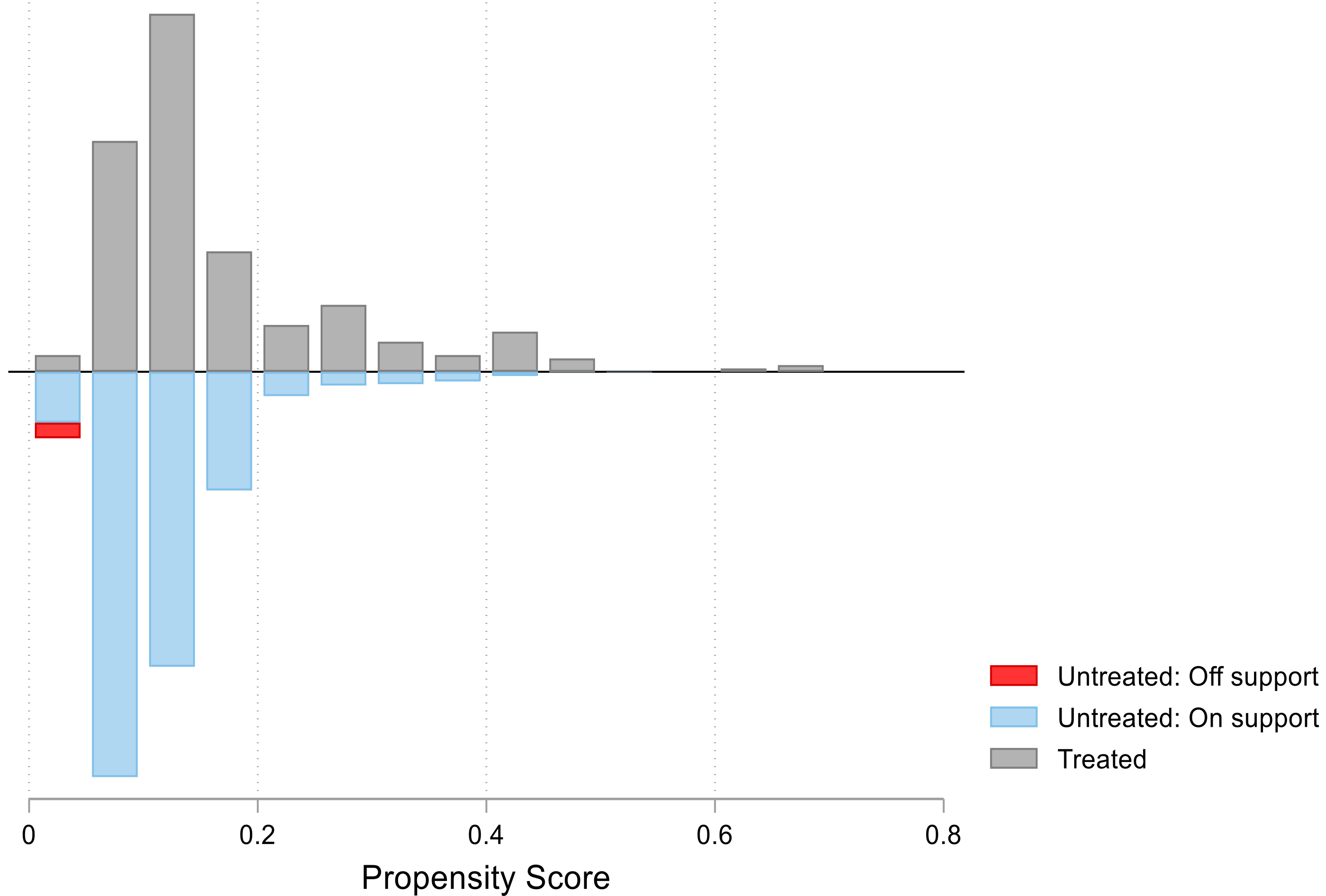
2.2.1. Propensity Score Matching
2.2.2. Linear Endogenous Treatment–Effect Model
2.2.3. Stochastic Metafrontier Approach
3. Results and Discussion
3.1. Determinants of Improved Maize Variety Adoption
3.2. Impact of Improved Maize Varieties on Productivity
3.3. Production Technology and Technical Efficiency Estimates
4. Conclusions and Policy Implications
Author Contributions
Funding
Institutional Review Board Statement
Informed Consent Statement
Data Availability Statement
Conflicts of Interest
Appendix A

| Variable | Coefficient | Std. Error |
|---|---|---|
| The proportion of improved growers | 4.735 *** | 0.238 |
| Land | −0.194 | 0.172 |
| Labor | −0.030 | 0.049 |
| Seed | 0.014 | 0.060 |
| Fertilizer | −0.010 | 0.020 |
| Chemical | 0.212 *** | 0.061 |
| Mixed cropping | −0.070 | 0.098 |
| Education | 0.075 * | 0.040 |
| Household size | 0.101 | 0.076 |
| Age | 0.009 | 0.160 |
| Soil quality | −0.206 * | 0.106 |
| Slope | −0.089 | 0.098 |
| Constant | −2.044 *** | 0.670 |
| Test for joint significance of IV | ||
| Athrho | −0.279 *** | |
| Chi-square | 12.85 *** | |
| Log Pseudo-likelihood | −3775.219 | |
| Observations | 2313 | |
| Conventional SPF Models | Selectivity-Corrected SPF Models | |||
|---|---|---|---|---|
| Variables | Pooled | Pooled | ||
| Coefficient | Std. Error | Coefficient | Std. Error | |
| Area | 1.240 *** | 0.063 | 1.206 *** | 0.061 |
| Labor | 0.298 *** | 0.026 | 0.286 *** | 0.025 |
| Seed | 1.037 *** | 0.021 | 1.042 *** | 0.021 |
| Fertilizer | −0.152 *** | 0.008 | −0.156 *** | 0.008 |
| Chemical | 0.959 *** | 0.023 | 0.958 *** | 0.022 |
| Area2 | −1.251 *** | 0.062 | −1.164 *** | 0.061 |
| Labor2 | −0.038 *** | 0.005 | −0.034 *** | 0.005 |
| Seed2 | −0.451 *** | 0.008 | −0.438 *** | 0.008 |
| Fertilizer2 | 0.216 *** | 0.002 | 0.216 *** | 0.002 |
| Chemical2 | 0.218 *** | 0.011 | 0.225 *** | 0.011 |
| Area × Labor | 0.049 *** | 0.011 | 0.045 *** | 0.010 |
| Area × Seed | 0.185 *** | 0.013 | 0.193 *** | 0.012 |
| Area × Fertilizer | −0.101 *** | 0.004 | −0.101 *** | 0.004 |
| Area × Chemical | −0.143 *** | 0.013 | −0.152 *** | 0.013 |
| Labor × Seed | 0.039 *** | 0.004 | 0.031 *** | 0.003 |
| Labor × Fertilizer | −0.030 *** | 0.001 | −0.029 *** | 0.001 |
| Labor × Chemical | −0.079 *** | 0.004 | −0.079 *** | 0.004 |
| Seed × Fertilizer | 0.008 *** | 0.002 | 0.007 *** | 0.002 |
| Seed × Chemical | −0.058 *** | 0.005 | −0.060 *** | 0.004 |
| Fertilizer × Chemical | −0.062 *** | 0.002 | −0.061 *** | 0.001 |
| Constant | 2.690 *** | 0.071 | 2.961 *** | 0.066 |
| 0.001 | 0.031 | 0.095 *** | 0.007 | |
| 0.120 *** | 0.002 | 0.102 *** | 0.003 | |
| Lambda | 0.004 | 0.031 | 0.929 *** | 0.009 |
| −0.086 *** | 0.004 | |||
| Log-likelihood | 1619.427 | 1683.292 | ||
| Observations | 2322 | 2322 | ||
References
- World Bank. World Development Report 2007; Agriculture for Development: Washington, DC, USA, 2006.
- Bezu, S.; Barrett, C.B.; Holden, S. Activity Choice in Rural Non-Farm Employment (RNFE): Survival Versus Accumulative Strategy (No. 11/14). Centre for Land Tenure Studies Working Paper; Norwegian University of Life Sciences (NMBU), Centre for Land Tenure Studies: Ås, Norway, 2014. [Google Scholar]
- Abdoulaye, T.; Wossen, T.; Awotide, B. Impacts of improved maize varieties in Nigeria: Ex-post assessment of productivity and welfare outcomes. Food Secur. 2018, 10, 369–379. [Google Scholar] [CrossRef]
- Badu-Apraku, B.; Fakorede, M.A.B. Maize in Sub-Saharan Africa: Importance and production constraints. In Advances in Genetic Enhancement of Early and Extra-Early Maize for Sub-Saharan Africa; Springer: Berlin/Heidelberg, Germany, 2017; pp. 3–10. [Google Scholar]
- McCann, J. Maize and grace: History, corn, and Africa’s new landscapes, 1500–1999. Comp. Stud. Soc. History 2001, 43, 246–272. [Google Scholar] [CrossRef] [Green Version]
- Macauley, H.; Ramadjita, T. Cereal crops: Rice, maize, millet, sorghum, wheat. In Proceedings of the Feeding Africa, Abdou Diouf International Conference Center, Dahar, Senegal, 21–23 October 2015; pp. 1–31. [Google Scholar]
- Bellon, M.R.; Taylor, J.E. “Folk’’ soil taxonomy and the partial adoption of new seed varieties. Econ. Dev. Cult. Change 1993, 41, 763–786. [Google Scholar] [CrossRef] [Green Version]
- Beza, E.; Silva, J.V.; Kooistra, L.; Reidsma, P. Review of yield gap explaining factors and opportunities for alternative data collection approaches. Eur. J. Agron. 2017, 82, 206–222. [Google Scholar] [CrossRef]
- Blanc, E. The impact of climate change on crop yields in Sub-Saharan Africa. Am. J. Clim. Change 2012, 01, 1–13. [Google Scholar] [CrossRef] [Green Version]
- Ringler, C.; Zhu, T.; Cai, X.; Koo, J.; Wang, D. The Impact of Irrigation on Nutrition, Health, and Gender: A Review Paper with Insights for Africa South of the Sahara; The International Food Policy Research Institute: Washington, DC, USA, 2010.
- Van Ittersum, M.K.; van Bussel, L.G.J.; Wolf, J.; Grassini, P.; van Wart, J.; Guilpart, N.; Claessens, L.; de Groot, H.; Wiebe, K.; Mason-D’Croz, D.; et al. Can sub-Saharan Africa feed itself? Proc. Natl. Acad. Sci. USA 2016, 113, 14964–14969. [Google Scholar] [CrossRef] [Green Version]
- Comin, D.; Hobijn, B. Cross-country technology adoption: Making the theories face the facts. J. Monet. Econ. 2004, 51, 39–83. [Google Scholar] [CrossRef] [Green Version]
- Ssozi, J.; Asongu, S.A. The comparative economics of catch-up in output per worker, total factor productivity, and technological gain in Sub-Saharan Africa. Afr. Dev. Rev. 2016, 28, 215–228. [Google Scholar] [CrossRef] [Green Version]
- Wossen, T.; Alene, A.; Abdoulaye, T.; Feleke, S.; Rabbi, I.Y.; Manyong, V. Poverty reduction effects of agricultural technology adoption: The case of improved cassava varieties in Nigeria. J. Agric. Econ. 2017, 70, 392–407. [Google Scholar] [CrossRef]
- Oyinbo, O.; Mbavai, J.J.; Shitu, M.B.; Kamara, A.Y.; Abdoulaye, T.; Ugbabe, O.O. Sustaining the beneficial effects of maize production in Nigeria: Does the adoption of short season maize varieties matters? Exp. Agric. 2019, 55, 885–894. [Google Scholar] [CrossRef]
- Ochinyabo, S. Rapid population growth and economic development issues in Nigeria. J. Econ. Allied Res. 2021, 6, 1–13. [Google Scholar]
- Faostat, F. FAOSTAT Statistical Database; FAO (Food and Agriculture Organization of the United Nations): Rome, Italy, 2022. [Google Scholar]
- Olaniyan, A.B. Maize: Panacea for hunger in Nigeria. Afr. J. Plant Sci. 2015, 9, 155–174. [Google Scholar] [CrossRef] [Green Version]
- Bamire, A.S.; Abdoulaye, T.; Sanogo, D.; Langyintuo, A. Characterization of Maize Producing Households in the Dry Savanna of Nigeria; CIMMYT: Ibadan, Nigeria, 2010. [Google Scholar]
- Ogbe, A.O.; Okoruwa, V.O.; Saka, O.J. Competitiveness of Nigerian rice and maize production ecologies: A policy analysis approach. Trop. Subtrop. Agroecosyst. 2011, 14, 493–500. [Google Scholar]
- Ammani, A.A. Trend analysis of maize production and productivity in Nigeria. J. Basic Appl. Res. Int. 2015, 2, 95–103. [Google Scholar]
- Agada, M.O.; Ajani, E.N. Constraints to increasing agricultural production and productivity among women farmers in sub-Saharan Africa: Implications for agricultural transformation agenda. Int. J. Agric. Sci. Res. Technol. Ext. Educ. Syst. 2014, 4, 143–150. [Google Scholar]
- Dedehouanou, S.F.A.; McPeak, J. Diversify more or less? Household income generation strategies and food security in rural Nigeria. J. Dev. Stud. 2020, 56, 560–577. [Google Scholar] [CrossRef]
- Dillon, A.; McGee, K.; Oseni, G. Agricultural production, dietary diversity, and climate variability. J. Dev. Stud. 2015, 51, 976–995. [Google Scholar] [CrossRef] [Green Version]
- Liverpool-Tasie, L.S.; Salau, S. Spillover Effects of Targeted Subsidies: An Assessment of Fertilizer and Improved Seed Use in Nigeria; International Food Policy Research Institute: Washington, DC, USA, 2013; Volume 1260, p. 32.
- Oyekale, A.S.; Idjesa, E. Adoption of improved maize seeds and production efficiency in Rivers State, Nigeria. Acad. J. Plant Sci. 2009, 2, 44–50. [Google Scholar]
- Tambo, J.A.; Abdoulaye, T. Climate change and agricultural technology adoption: The case of drought tolerant maize in rural Nigeria. Mitig. Adapt. Strateg. Glob. Change 2012, 17, 277–292. [Google Scholar] [CrossRef]
- Diagne, A.; Kinkingninhoun-Medagbe, F.M.; Ojehomon, V.T.; Abedayo, S.B.; Amovin-Assagba, E.; Nakelse, T. Assessing the Diffusion and Adoption of Improved Rice Varieties in Nigeria. Diffusion and Improved Varieties in Africa (DIIVA)-Objective 2 Report; IITA: Ibadan, Nigeria, 2013. [Google Scholar]
- Alene, A.D.; Mwalughali, J. Adoption of Improved Cassava Varieties in Southwestern Nigeria, Objective 2 Technical Report; International Institute of Tropical Agriculture (IITA): Lilongwe, Malawi, 2012. [Google Scholar]
- Abro, Z.A.; Jaleta, M.; Qaim, M. Yield effects of rust-resistant wheat varieties in Ethiopia. Food Secur. 2017, 9, 1343–1357. [Google Scholar] [CrossRef]
- Hurley, T.; Koo, J.; Tesfaye, K. Weather risk: How does it change the yield benefits of nitrogen fertilizer and improved maize varieties in sub-Saharan Africa? Agric. Econ. 2018, 49, 711–723. [Google Scholar] [CrossRef] [Green Version]
- Greene, W.A. Stochastic frontier model with correction for sample selection. J. Product. Anal. 2010, 34, 15–24. [Google Scholar] [CrossRef] [Green Version]
- Huang, C.J.; Huang, T.H.; Liu, N.H. A new approach to estimating the metafrontier production function based on a stochastic frontier framework. J. Product. Anal. 2014, 42, 241–254. [Google Scholar] [CrossRef]
- Villano, R.; Bravo-Ureta, B.; Solís, D.; Fleming, E. Modern rice technologies and productivity in the Philippines: Disentangling technology from managerial gaps. J. Agric. Econ. 2015, 66, 129–154. [Google Scholar] [CrossRef] [Green Version]
- Khandker, S.R.; Samad, G.B.; Koolwal, H.A. Handbook on Impact Evaluation Quantitative Methods and Practices; World Bank Publication: Washington, DC, USA, 2010.
- Di Falco, S.; Veronesi, M. How can African agriculture adapt to climate change? A counterfactual analysis from Ethiopia. Land Econ. 2013, 89, 743–766. [Google Scholar] [CrossRef] [Green Version]
- Di Falco, S.; Veronesi, M.; Yesuf, M. Does adaptation to climate change provide food security? A micro-perspective from Ethiopia. Am. J. Agric. Econ. 2011, 93, 825–842. [Google Scholar] [CrossRef] [Green Version]
- Shiferaw, B.; Kassie, M.; Jaleta, M.; Yirga, C. Adoption of improved wheat varieties and impacts on household food security in Ethiopia. Food Policy 2014, 44, 272–284. [Google Scholar] [CrossRef]
- Battese, G.E.; Prasada Rao, D.S.; O’Donnell, C.J. A metafrontier production function for estimation of technical efficiencies and technology gaps for firms operating under different technologies. J. Product. Anal. 2004, 21, 91–103. [Google Scholar] [CrossRef]
- Chang, B.G.; Huang, T.H.; Kuo, C.Y. A comparison of the technical efficiency of accounting firms among the US, China, and Taiwan under the framework of a stochastic metafrontier production function. J. Product. Anal. 2015, 44, 337–349. [Google Scholar] [CrossRef]
- Martinez Cillero, M.; Wallace, M.; Thorne, F.; Breen, J. Analyzing the impact of subsidies on beef production efficiency in selected European Union Countries. A stochastic metafrontier approach. Am. J. Agric. Econ. 2021, 103, 1903–1923. [Google Scholar] [CrossRef]
- O’Donnell, C.J.; Rao, D.S.P.; Battese, G.E. Metafrontier frameworks for the study of firm-level efficiencies and technology ratios. Empir. Econ. 2008, 34, 231–255. [Google Scholar] [CrossRef]
- Kumbhakar, S.C.; Wang, H.; Horncastle, A.P. A Practitioner’s Guide to Stochastic Frontier Analysis Using Stata; Cambridge University Press: New York, NY, USA, 2015. [Google Scholar]
- Bravo-Ureta, B.E.; Greene, W.; Solís, D. Technical efficiency analysis correcting for biases from observed and unobserved variables: An application to a natural resource management project. Empir. Econ. 2012, 43, 55–72. [Google Scholar] [CrossRef]
- Zegeye, T.; Tadesse, B.; Tesfaye, S. Determinants of adoption of improved maize technologies in major maize growing regions in Ethiopia. In Proceedings of the Second National Maize Workshop of Ethiopia, EARO, Addis Abeda, Ethiopia, 12–16 November 2001; pp. 125–136. [Google Scholar]
- Leuven, E.; Sianesi, B. PSMATCH2: STATA module to perform full Mahalanobis and propensity score matching, common support graphing, and covariate imbalance testing. Bost. Coll. Dep. Econ. Stat. Softw. Compon. Ser. 2003, S432001. [Google Scholar]
- Bravo-Ureta, B.E.; Almeida, A.N.; Solís, D.; Inestroza, A. The economic impact of marena’s investments on sustainable agricultural systems in Honduras. J. Agric. Econ. 2011, 62, 429–448. [Google Scholar] [CrossRef]
- Pufahl, A.; Weiss, C.R. Evaluating the effects of farm programmes: Results from propensity score matching. Eur. Rev. Agric. Econ. 2009, 36, 79–101. [Google Scholar] [CrossRef] [Green Version]
- Kodde, F.C.; Palm, D.A. Wald criteria for jointly testing equality and inequality restrictions. Econom. J. Econom. Soc. 1986, 54, 1243–1248. [Google Scholar] [CrossRef]
- Bravo-Ureta, B.E.; González-Flores, M.; Greene, W.; Solís, D. Technology and technical efficiency change: Evidence from a difference in differences selectivity corrected stochastic production frontier model. Am. J. Agric. Econ. 2021, 103, 362–385. [Google Scholar] [CrossRef]
- Ma, W.; Renwick, A.; Yuan, P.; Ratna, N. Agricultural cooperative membership and technical efficiency of apple farmers in China: An analysis accounting for selectivity bias. Food Policy 2018, 81, 122–132. [Google Scholar] [CrossRef]
- Abdul-Rahaman, A.; Abdulai, A. Do farmer groups impact on farm yield and efficiency of smallholder farmers? Evidence from rice farmers in northern Ghana. Food Policy 2018, 81, 95–105. [Google Scholar] [CrossRef]
- Zheng, H.; Ma, W.; Wang, F.; Li, G. Does internet use improve technical efficiency of banana production in China? Evidence from a selectivity-corrected analysis. Food Policy 2021, 102, 102044. [Google Scholar] [CrossRef]
- Beaman, L.; Karlan, D.; Thuysbaert, B.; Udry, C. Profitability of fertilizer: Experimental evidence from female rice farmers in Mali. Am. Econ. Rev. 2013, 103, 381–386. [Google Scholar] [CrossRef] [Green Version]
- Sheahan, M.; Barrett, C.B. Ten striking facts about agricultural input use in Sub-Saharan Africa. Food Policy 2017, 67, 12–25. [Google Scholar] [CrossRef] [PubMed] [Green Version]
| Variables | Definition | Mean | Std. Dev. |
|---|---|---|---|
| Variables used in PSM and Probit Model | |||
| Variety type | 1 if farmers grow improved varieties on the farm plot, 0 otherwise | 0.118 | 0.322 |
| Gender | 1 if farmer is male, 0 otherwise | 0.826 | 0.379 |
| Age | Age of the household head in years (Years) | 50.302 | 14.932 |
| Education | Number of years of formal education of household head (Years) | 5.396 | 5.185 |
| Household size | Number of family members | 6.743 | 3.908 |
| Wealth index | Wealth index (NGN 1000) | 183.148 | 150.812 |
| Farm size | Total crop area planted in hectares (Hectares) | 0.544 | 0.587 |
| Soil quality | 1 if farm plot soil is good, 0 otherwise | 0.833 | 0.373 |
| Mixed cropping | 1 if crops is under mixed cropping, 0 otherwise | 0.708 | 0.455 |
| Plot slope | 1 if farm plot is flat, 0 otherwise | 0.756 | 0.429 |
| Access to extension agent | 1 if farmer attended training session on improved varieties, 0 otherwise | 0.065 | 0.247 |
| Credit access | 1 if the farmer has access to credit | 0.151 | 0.358 |
| Participation in non-farm enterprise | 1 if the farmer participated in non-farm enterprise, 0 otherwise | 0.505 | 0.500 |
| Use machine on plots | 1 if the farmer uses machine or implement on the farm plot, 0 otherwise | 0.101 | 0.301 |
| Use inorganic fertilizer on plot | 1 if the farmer uses inorganic fertilizers on the plot, 0 otherwise | 0.452 | 0.498 |
| Variables used in the SPF models | |||
| Output | Total production of corps in kilograms | 518.472 | 691.117 |
| Seed | Seed used in kilograms | 6.606 | 8.285 |
| Fertilizer | Total NPK and Urea (kilograms of active ingredient) | 61.199 | 99.929 |
| Chemical | Total active ingredients of chemical used in kilograms | 2.099 | 2.964 |
| Labor | Total labor used in crop production (worker/hour) | 385.495 | 380.692 |
| Share adopting | Proportion of household in enumeration area | 0.117 | 0.191 |
| Improved varieties | 1 if the plot is planted improved varieties, 0 otherwise | 0.118 | 0.322 |
| Number of observations | 2519 | ||
| Unmatched Sample | Matched Sample | |||||
|---|---|---|---|---|---|---|
| Variables | Improved | Traditional | Diff. | Improved | Traditional | Diff. |
| Gender | 0.882 | 0.818 | 0.063 *** | 0.905 | 0.885 | 0.020 |
| Age | 47.439 | 50.683 | −3.244 *** | 47.401 | 47.550 | −0.149 |
| Education | 5.747 | 4.991 | 0.756 *** | 5.989 | 6.035 | −0.045 |
| Household size | 7.236 | 6.677 | 6.743 ** | 7.243 | 7.657 | −0.414 |
| Wealth index | 193.674 | 181.747 | 11.927 *** | 192.838 | 161.172 | 31.666 ** |
| Credit access | 0.162 | 0.149 | 0.013 | 0.148 | 0.142 | 0.006 |
| Access to extension agent | 0.175 | 0.050 | 0.126 *** | 0.176 | 0.094 | 0.082 |
| Soil quality | 0.760 | 0.843 | −0.082 *** | 0.768 | 0.779 | −0.011 |
| Plot slope | 0.706 | 0.763 | −0.057 ** | 0.701 | 0.692 | 0.009 |
| Mixed cropping | 0.605 | 0.722 | −0.117 *** | 0.609 | 0.578 | 0.031 |
| Participation in non-farm enterprise | 0.578 | 0.496 | 0.082 *** | 0.581 | 0.542 | 0.039 |
| Use machine on plots | 0.142 | 0.095 | 0.047 ** | 0.148 | 0.114 | 0.034 |
| Use inorganic fertilizer on plot | 0.530 | 0.441 | 0.089 *** | 0.535 | 0.528 | 0.007 |
| North | 0.693 | 0.562 | 0.131*** | 0.701 | 0.702 | 0.002 |
| Production | 695.055 | 494.960 | 200.095*** | 701.812 | 623.346 | 78.466 |
| Farm size | 0.644 | 0.537 | 0.107 *** | 0.643 | 0.634 | 0.009 |
| Labor | 349.708 | 390.260 | −40.552 * | 350.212 | 367.699 | −17.487 |
| Seed | 8.284 | 6.284 | 1.901 *** | 8.410 | 7.965 | 0.446 |
| Fertilizer | 86.127 | 57.880 | 28.247 *** | 88.516 | 75.571 | 12.282 |
| Chemical | 3.095 | 1.967 | 1.128 *** | 3.137 | 2.439 | 0.698 |
| Number of observations | 296 | 2223 | 281 | 2041 | ||
| Matched Sample | Unmatched Sample | |||
|---|---|---|---|---|
| Variables | Coefficient | Std. Error | Coefficient | Std. Error |
| Gender | 0.031 | 0.118 | 0.048 | 0.117 |
| Age | −0.005 * | 0.003 | −0.006 ** | 0.003 |
| Education | 0.007 | 0.007 | 0.008 | 0.007 |
| Household size | 0.023 ** | 0.011 | 0.025 ** | 0.011 |
| Wealth index | 0.226 *** | 0.071 | 0.243 *** | 0.071 |
| Farm size | 0.022 | 0.067 | 0.024 | 0.066 |
| Credit access | −0.006 | 0.099 | −0.010 | 0.099 |
| Access to extension agent | 0.657 *** | 0.115 | 0.681 *** | 0.114 |
| Soil quality | −0.223 ** | 0.088 | −0.230 *** | 0.088 |
| Plot slope | −0.135 * | 0.079 | −0.140 * | 0.079 |
| Mixed cropping | −0.128 | 0.083 | −0.137 * | 0.082 |
| Participation in non-farm enterprise | 0.119 | 0.072 | 0.118 | 0.072 |
| Use machine on plots | 0.104 | 0.109 | 0.122 | 0.108 |
| Use inorganic fertilizer on plot | 0.040 | 0.076 | 0.045 | 0.076 |
| North | 0.183 * | 0.103 | 0.180 * | 0.103 |
| Constant | −3.760 *** | 0.904 | −3.960 *** | 0.894 |
| Log-likelihood function | −811.987 | −815.022 | ||
| Chi-squared test statistic | 89.41 | 104.77 | ||
| Number of observations | 2322 | 2519 | ||
| Yield (kg/ha) | ATT | Std. Error |
|---|---|---|
| Propensity score matching × | ||
| Kernel | 0.215 ** | 0.091 |
| Radius | 0.213 *** | 0.086 |
| Stratification | 0.138 * | 0.084 |
| Linear endogenous treatment effect † | ||
| Yield (kg/ha) | 0.387 *** | 0.106 |
| Conventional SPF Models | Selectivity-Corrected SPF Models | |||||||
|---|---|---|---|---|---|---|---|---|
| Variables | Improved | Traditional | Improved | Traditional | ||||
| Coefficient | Std. Error | Coefficient | Std. Error | Coefficient | Std. Error | Coefficient | Std. Error | |
| Area | −0.967 | 1.431 | 1.638 *** | 0.508 | −0.958 | 1.431 | 1.648 *** | 0.508 |
| Labor | 0.124 | 0.667 | 0.251 | 0.204 | 0.144 | 0.666 | 0.252 | 0.204 |
| Seed | 1.880 *** | 0.527 | 0.987 *** | 0.173 | 1.881 *** | 0.527 | 0.970 *** | 0.173 |
| Fertilizer | −0.448 *** | 0.174 | −0.135 ** | 0.066 | −0.433 ** | 0.174 | −0.140 ** | 0.066 |
| Chemical | 1.079 ** | 0.531 | 0.910 *** | 0.185 | 0.984 * | 0.532 | 0.925 *** | 0.185 |
| Area2 | −0.500 | 1.381 | −1.472 ** | 0.505 | −0.439 | 1.378 | −1.468 *** | 0.500 |
| Labor2 | −0.007 | 0.134 | −0.027 | 0.038 | 0.001 | 0.134 | −0.026 | 0.038 |
| Seed2 | −0.373 ** | 0.158 | −0.458 *** | 0.063 | −0.365 ** | 0.158 | −0.451 *** | 0.063 |
| Fertilizer2 | 0.223 *** | 0.051 | 0.213 *** | 0.019 | 0.216 *** | 0.051 | 0.213 *** | 0.019 |
| Chemical2 | 0.240 | 0.223 | 0.211 ** | 0.091 | 0.214 | 0.223 | 0.213 ** | 0.091 |
| Area × Labor | 0.393 * | 0.235 | −0.021 | 0.085 | 0.384 | 0.234 | −0.024 | 0.086 |
| Area × Seed | −0.540 ** | 0.274 | 0.308 *** | 0.106 | −0.563 ** | 0.274 | 0.313 *** | 0.105 |
| Area × Fertilizer | −0.064 | 0.095 | −0.119 *** | 0.035 | −0.068 | 0.093 | −0.121 *** | 0.035 |
| Area × Chemical | 0.517 ** | 0.286 | 0.185 * | 0.103 | 0.578 ** | 0.289 | −0.187 * | 0.103 |
| Labor × Seed | −0.095 | 0.095 | 0.040 | 0.029 | −0.094 | 0.095 | 0.040 | 0.029 |
| Labor × Fertilizer | 0.030 | 0.031 | −0.033 *** | 0.010 | 0.029 | 0.031 | −0.032 *** | 0.010 |
| Labor × Chemical | −0.218 ** | 0.091 | −0.056 * | 0.032 | −0.205 ** | 0.091 | −0.059 * | 0.032 |
| Seed × Fertilizer | −0.012 | 0.032 | 0.014 | 0.013 | −0.012 | 0.032 | 0.013 | 0.013 |
| Seed × Chemical | 0.079 | 0.093 | −0.087 ** | 0.037 | 0.084 | 0.094 | −0.086 ** | 0.037 |
| Fertilizer × Chemical | −0.090 *** | 0.031 | −0.056 *** | 0.012 | −0.088 *** | 0.031 | −0.056 *** | 0.012 |
| Constant | 3.363 ** | 1.668 | 2.749 *** | 0.535 | 3.457 ** | 1.668 | 2.912 *** | 0.542 |
| 0.948 *** | 0.184 | 0.968 *** | 0.071 | 0.937 *** | 0.187 | 0.959 | 0.073 | |
| 0.656 *** | 0.088 | 0.718 *** | 0.033 | 0.657 *** | 0.088 | 0.721 *** | 0.033 | |
| Lambda | 1.445 *** | 0.264 | 1.349 *** | 0.101 | 1.427 *** | 0.266 | 1.330 *** | 0.102 |
| −0.117 | 0.085 | −0.077 * | 0.041 | |||||
| Log-likelihood | −357.586 | −2727.073 | −356.634 | −2725.329 | ||||
| Observations | 281 | 2041 | 281 | 2041 | ||||
| Selectivity-Corrected SPF Models | Conventional SPF Models | |||||
|---|---|---|---|---|---|---|
| Item | Improved | Traditional | Metafrontier | Improved | Traditional | Metafrontier |
| TGR efficiency | ||||||
| Mean | 0.905 | 0.733 | 0.830 | 0.999 | 0.896 | 0.896 |
| Standard Deviation | 0.072 | 0.009 | 0.028 | 0.182 | 0.182 | 0.180 |
| Minimum | 0.562 | 0.674 | 0.562 | 0.996 | 0.810 | 0.810 |
| Maximum | 0.991 | 0.958 | 0.991 | 0.999 | 0.999 | 0.999 |
| Technical efficiency | ||||||
| Mean | 0.543 | 0.536 | 0.536 | 0.540 | 0.533 | 0.534 |
| Standard Deviation | 0.150 | 0.146 | 0.147 | 0.152 | 0.148 | 0.148 |
| Minimum | 0.064 | 0.028 | 0.028 | 0.062 | 0.027 | 0.026 |
| Maximum | 0.862 | 0.859 | 0.862 | 0.863 | 0.861 | 0.863 |
| MTE efficiency | ||||||
| Mean | 0.491 | 0.393 | 0.445 | 0.540 | 0.478 | 0.477 |
| Standard Deviation | 0.141 | 0.136 | 0.137 | 0.152 | 0.148 | 0.148 |
| Minimum | 0.059 | 0.027 | 0.027 | 0.062 | 0.026 | 0.027 |
| Maximum | 0.844 | 0.800 | 0.844 | 0.863 | 0.863 | 0.863 |
Disclaimer/Publisher’s Note: The statements, opinions and data contained in all publications are solely those of the individual author(s) and contributor(s) and not of MDPI and/or the editor(s). MDPI and/or the editor(s) disclaim responsibility for any injury to people or property resulting from any ideas, methods, instructions or products referred to in the content. |
© 2023 by the authors. Licensee MDPI, Basel, Switzerland. This article is an open access article distributed under the terms and conditions of the Creative Commons Attribution (CC BY) license (https://creativecommons.org/licenses/by/4.0/).
Share and Cite
Olasehinde, T.S.; Qiao, F.; Mao, S. Impact of Improved Maize Varieties on Production Efficiency in Nigeria: Separating Technology from Managerial Gaps. Agriculture 2023, 13, 611. https://doi.org/10.3390/agriculture13030611
Olasehinde TS, Qiao F, Mao S. Impact of Improved Maize Varieties on Production Efficiency in Nigeria: Separating Technology from Managerial Gaps. Agriculture. 2023; 13(3):611. https://doi.org/10.3390/agriculture13030611
Chicago/Turabian StyleOlasehinde, Toba Stephen, Fangbin Qiao, and Shiping Mao. 2023. "Impact of Improved Maize Varieties on Production Efficiency in Nigeria: Separating Technology from Managerial Gaps" Agriculture 13, no. 3: 611. https://doi.org/10.3390/agriculture13030611
APA StyleOlasehinde, T. S., Qiao, F., & Mao, S. (2023). Impact of Improved Maize Varieties on Production Efficiency in Nigeria: Separating Technology from Managerial Gaps. Agriculture, 13(3), 611. https://doi.org/10.3390/agriculture13030611