Article

Delineating Natural Terroir Units in Wine Regions Using Geoinformatics

by
Nikolaos Karapetsas
1,
Thomas K. Alexandridis
1,*,
George Bilas
1,
Serafeim Theocharis
2 and
Stefanos Koundouras
2
1
Laboratory of Remote Sensing, Spectroscopy and Geographic Information Systems, Department of Hydraulics, Soil Science and Agricultural Engineering, School of Agriculture, Aristotle University of Thessaloniki, 54124 Thessaloniki, Greece
2
Laboratory of Viticulture, Department of Horticulture, School of Agriculture, Aristotle University of Thessaloniki, 54124 Thessaloniki, Greece
*
Author to whom correspondence should be addressed.
Agriculture 2023, 13(3), 629; https://doi.org/10.3390/agriculture13030629
Submission received: 16 January 2023 / Revised: 1 March 2023 / Accepted: 4 March 2023 / Published: 6 March 2023

Abstract

:
The terroir effect refers to the interactions between the grapes and their natural surroundings and has been recognized as an important factor in wine quality. The identification and mapping of viticultural terroir have long been relying on expert opinion coupled with land classification and soil/climate mapping. In this study, the data-driven approach has been implemented for mapping natural terroir units based on spatial modeling of public-access geospatial information regarding the three most important environmental factors that make up the terroir effect on different scales, climate, soil, and topography. K-means cluster analysis was applied to the comprehensive databases of relevant spatial information, and the optimum number of clusters was identified by the Dunn and CCC indices. The results have revealed ten clusters that cover the agricultural area of Drama (Greece), where it was applied, and displayed variable conditions on the climate, soil, and topographic factors. The implications of the resulting natural terroir units on the vini-viticultural management of the most common vine varieties are discussed. As more accurate and detailed input spatial data become available, the potential of such an approach is highlighted and paving the way toward a true understanding of the drivers of terroir.

1. Introduction

Terroir is a concept that includes climatic, topographical, geological, and pedological factors, as well as traditional vine varieties and vine farmers’ expertise. Terroir was defined as a “complex of natural environmental elements, which cannot simply be modified by the producer” [1]. Several authors have shown how environmental conditions affect the content and quality of grapes [2,3]. Numerous studies have demonstrated that the terroir effect on grapes and wine is mostly explained by physical and climatic conditions [2,4]. The current official definition of viticultural terroir by the International Organization of Vine and Wine (O.I.V.) states that “terroir is a concept which refers to an area in which collective knowledge of the interactions between the identifiable physical and biological environment and applied viti-vinicultural practices develop, providing distinctive characteristics for the products originating from this area”. Specific soil, terrain, temperature, landscape, and biodiversity traits are all elements of terroir. The idea of “Natural Terroir Units”, or NTUs, was put into practice by Priori, et al. [5]. They defined an NTU as “a volume of the Earth’s biosphere that is characterized by a stable group of values relating to the topography, climate, substrate, and soil”.
The identification of NTUs has traditionally relied upon expert opinion on wine production and related environmental factors, coupled with standard approaches to land classification based on thematic mapping of soil and climatic conditions. The derived terroir units are usually based on pre-defined boundaries of administrative districts or patterns derived from surface hydrology, road, or railway networks [6]. Moreover, the relative importance of soil, climatic, and topographic parameters on wine production are purely based on qualitative expert opinion. As a consequence, expert approaches tend to validate pre-existing terroirs defined historically, through modern GIS applications, with a minimum contribution toward the understanding of the true drivers of terroir [7].
Rather than employing expert opinion in the identification of Natural Terroir Units (NTUs), the data-driven approach is solely based on quantitative geospatial analysis of exhaustive databases of soil, climatic, and topographic information. Spatial and temporal variation in geographical data is taken into account in an effort to identify the similarities in the patterns of variations between the input environmental variables, which are usually revealed with clustering techniques or similar classification methods [6]. All data sources originate from online platforms of public-access geospatial information, delivered in many different spatial resolutions and data formats, with global or regional coverage, concerning the three major and most commonly used groups of terroir-related environmental factors, soil, climate, and topography.
Soil is one of the most crucial elements in viticulture since it is a component of terroir. Grapevine composition and, in turn, wine quality can be influenced by the texture, structure, and chemistry of the soil [8]. Compact and shallow soils can prevent roots from accessing water and nutrients, restricting root development. Additionally, soil water retention properties can impact grapevine performance and are considered strongly important [9]. In Mediterranean regions, where grapevines are typically subjected to significant heat extremes and water deficiency, soil water storage capacity is highly critical [10].
An essential factor influencing the formation and growth of grapevines is climate, which has a big impact on vine physiological functions during its typical growing season, from April to September. Grapevine phenology is closely related to the current atmospheric conditions, affecting grapevine yield, wine output, and quality [11,12,13]. All these environmental factors define suitability for a certain variety or type of wine, limiting the geographic range of grapevine [14].
Another important component that affects a region’s viticultural traits is its topographic landscape features which interact with soil and climate factors. Elevation, slope, and aspect or exposure are the most critical topographic factors for viticulture [11]. Site and variety selection are strongly influenced by elevation’s effects on vineyard temperatures [9]. Terrain slope affects canopy microclimate through solar exposure, soil erosion, water drainage, and viticultural management. The terrain aspect involves the surface net incoming solar radiation flow and is a crucial factor in site selection [15].
Several researchers have argued that the terroir effect on wine’s qualitative qualities, such as its aromas and flavors, is ambiguous and challenging to explain scientifically [16]. It is possible to say that the grapevine variety expresses the influence of climate, soil, and geography. Despite certain similarities among varieties, each has unique qualitative characteristics, including aromatic composition. The terroir effect should therefore be taken into account separately for each variety and wine style.
Multivariate spatial and temporal modeling of climatic, soil, and agronomic features is usually required for the identification and mapping of locations with high-quality grape and wine production [17,18]. Latest technologies and analytical methods enable the recording and processing of detailed spatial and temporal information on terroir-related environmental factors, assisting this way in the development of comprehensive spatial models for delineating terroir units and forecasting their viticultural response. Spatial modeling of winegrowing terroirs is facilitated by the use of the latest generation of geospatial technologies, including remote and proximal sensing [7]. Since the early 2000s, a considerable volume of research has focused on terroir zoning, and numerous viticultural target properties have been taken into consideration, with a primary focus on grape and canopy characteristics, yield, or biomass and a secondary focus on soil parameters at the within-field scale [7].
Mapping terroir units on a regional scale involves analysis of earth observation data in order to support the monitoring of phenology and status of the vines across various individual fields dispersed throughout a regional viticultural area and assist the decisions concerning the most suitable plant material locally. An adaptation of the terroir idea from remote sensing to spatial modeling includes soil landscape units as the fundamental building blocks for terroir unit delineation, accompanied by the climate and grape composition data [18]. Although more complex spatial models using auxiliary spatial information, such as kriging with hyperspectral imagery [19], have also been developed, geostatistical approaches and primarily kriging based on primary spatial information, such as yield or ECa, are the most popular methods used in terroir-related studies [20]. Following the use of a number of geostatistical models, k-means cluster analysis is commonly carried out in the viticultural regions to identify the NTU-based viticultural terroir units [21].
The objective of the current study was to establish a data-driven approach toward NTU zoning, which was tested in the wine production of Drama (Greece). The approach was based on public-access data pools of geospatial information regarding physical and chemical properties related to soil and climatic and topographic characteristics of the wine-production environment.

2. Materials and Methods

2.1. Study Area

Despite the historical background of Drama Regional Unit (Greece) related to wine-making, it was not until the late 1970s and early 1980s that systematic wine production was revived, leaving its own characteristic footprint on Greek and international wine scenery ever since. Although no Protected Designation of Origin (PDO) area has been established in Drama, it is widely acknowledged as one of the most significant viticultural regions of Greece. The continental climate of the area (characterized by the cool nighttime temperatures) related to its isolation from the sea by the three surrounding mountains of Pangeon, Falakro, and Menikio, creates ideal conditions for the acclimatization of the early-harvest, white and red varieties, most notably international ones. Major wine grape varieties cultivated in the region with the aim of producing high-quality wines are the white varieties Sauvignon blanc and the red varieties Cabernet Sauvignon and Merlot. Recently, Greek varieties, such as the white Assyrtiko and the red Agiorgitiko, have been introduced in the area. Vineyards are scattered mainly across the central and southern parts of the region, at altitudes up to 500 m, covering approximately 500 ha, and the total annual wine production is estimated at around 3M bottles.
The study area is presented in Figure 1. The region is characterized by a mountainous landscape, mainly in the central and northernmost parts, with elevation reaching up to 2200 m. Natural vegetation and forests are the dominant land cover type in the northern mountainous part of the region (except for a few plateaus dedicated to agriculture), while the southern area of the region is governed by agricultural land cover in the plain lower parts. The average annual precipitation in the plain of Drama exceeds 540 mm, mainly concentrated during winter. Clay and clay–loam soils, with a high cation exchange capacity (CEC), dominate the southern plain, while sandy loams occupy the northwestern plateau of Kato Nevrokopi. From the total area of Drama Regional Unit, the study area included only the agricultural land, which was used as an analysis mask in the consequent data processing for the identification of NTUs. The final study area covered an area of approximately 69.7 K ha, mostly scattered across the southern and western parts of Drama Regional Unit.

2.2. Data Sources

The identification of NTUs was based on a comprehensive establishment of a geographical database populated with geodata from public-access geospatial information concerning land cover, soil, climate, and topography.
The complete list of the geospatial data utilized for terroir zoning is presented in Table 1, along with their statistical distribution constrained by the analysis mask of the study area, i.e., the agricultural land cover. All data were retrieved in the form of spatial raster datasets from the following online sources:
  • Copernicus Land Monitoring Service (ver.3). Land Cover Change Version 3.0 product at 100 m resolution. The Copernicus Global Land Service (CGLS) systematically produces a series of qualified bio-geophysical products on a regular basis, at a global scale and at mid to low spatial resolution (https://land.copernicus.eu/global/products/lc, accessed on 30 November 2022). Land cover from CGLS was used for the purpose of masking the area of interest to the agricultural land cover class;
  • Copernicus Sentinel-2 MSI Data supporting the monitoring of vegetation from the online GEE platform (https://developers.google.com/earth-engine/datasets/catalog/COPERNICUS_S2_SR_HARMONIZED#description, accessed on 30 November 2022);
  • European Digital Elevation Model (EU-DEM), version 1.1. The EU-DEM v1.1 is a contiguous dataset, distributed and divided into 1000 km × 1000 km tiles, at 25 m resolution, in geotiff 32-bit format (https://land.copernicus.eu/imagery-in-situ/eu-dem/, accessed on 30 November 2022);
  • SoilGrids. SoilGrids is a system for digital soil mapping service based on a global compilation of soil profile data (WoSIS) and environmental layers [22]. SoilGrids delivers global predictions at 250 m resolution for standard numeric soil properties at seven standard depths, in addition to the distribution of soil classes distribution, based on the World Reference Base (WRB) and USDA classification systems (https://data.isric.org/geonetwork/srv/eng/catalog.search, accessed on 30 November 2022);
  • EU-SoilHydroGrids ver. 1.0. EU-SoilHydroGrids ver1.0 provides soil hydrological data with full continental coverage. The multilayered European Soil Hydraulic Database (EU-SoilHydroGrids ver1.0) was derived via European pedotransfer functions (EU-PTFs) based on the soil information of SoilGrids250 m and aggregated 1 km resolution datasets (https://esdac.jrc.ec.europa.eu/content/3d-soil, accessed on 30 November 2022) [22,23];
  • Climate Data Store. European Centre for Medium-Range Weather Forecasts (ECMWF) is producing an enhanced global dataset concerning the land component of the fifth generation of European Re-Analysis (ERA5), referred to as ERA5-Land. Climatic data concerning temperature, precipitation, evapotranspiration, wind speed, and incoming solar radiation were accessed in the form of time-series averages for the time period of 2002–2022, extracted from monthly averaged data for all climatic variables besides heat frequency, which resulted from hourly analysis data. (https://cds.climate.copernicus.eu/cdsapp, accessed on 30 November 2022).

2.3. Cluster Analysis

2.3.1. K-means Clustering

K-means clustering was performed on the multivariate datasets using the Hartigan and Wong clustering algorithm, which is one of the most widely used k-means techniques [24]. It belongs to partitioning-based grouping techniques, which are based on the iterative relocation of data points between clusters. Their goal is to produce clusters of cases/variables with a high degree of similarity within each group and a low degree of similarity between groups. The algorithm searches for the partition of data space with the locally optimal within-cluster sum of squares of errors, meaning that it may re-assign a case to another cluster, even if it belongs to the cluster of the closest centroid if doing so minimizes the total within-cluster sum of squares [25]. Although popular due to ease of implementation, simplicity, efficiency, and empirical success, the primary drawback of k-means is that it rarely achieves global optimization for centroid location [26,27]. The k-means algorithms are local search heuristics and are, therefore, sensitive to the initial centroids chosen [28]. To counteract for this limitation, multiple applications of the technique were applied with different initialization cases to obtain a more stable solution for k-means clustering.

2.3.2. Optimal Number of Clusters

Determining the optimal number of clusters in the data set of environmental parameters is a fundamental issue in partitioning clustering, i.e., k-means clustering, where the user is required to pre-specify the number of k-clusters to be generated. The k-means algorithm divides the total squared distance between each data point and its closest cluster mean into k-clusters (centroid). As a result, the process initialization has a significant impact on the k-means result [26]. Misplaced initialization can cause the iterations to get stuck into an inferior local minimum. The Dunn index is a method for internal evaluation that is essentially equivalent to the ratio of intra-cluster to inter-cluster similarity [29]. As the objective was compact clusters, the solution with the highest Dunn index was employed for cluster discrimination. The Cubic Clustering Criterion (CCC) is another statistical index provided by the SAS Institute [30]. The maximum value of the index was used to indicate the optimal number of clusters in the data set.
Dunn and CCC indices were evaluated individually by comparing several clustering structures resulting from the k-means algorithm with different parameter values, i.e., the number of clusters. To ensure the robustness of this approach, due to the inherent randomization of the k-means algorithm, several repetitions of the comparative process, individually for Dunn and CCC indices, are required.

2.3.3. Cluster Validation

Clustering validation has long been acknowledged as one of the critical issues related to the success of clustering applications since clustering methods tend to generate clusters even for relatively homogeneous data sets [25]. Cluster analysis is frequently performed in an experimental way, and thus, the patterns it uncovers are not always significant. Either for external or internal types, clustering validation may vary depending on whether or not independent data are used for clustering validation [31]. Since no prior information regarding historically established viticultural terroir zoning in Drama region existed, internal validation was initially carried out based entirely on data information.
A primary issue related to clustering is its stability or consistency, which is assessed using the observed variation between clustering results over different subsamples drawn from the input data [27]. Stability in cluster analysis is strongly related to inherent data properties, weakened by lack of robustness of the clustering method or unsuitable clustering method, which is inadequate for the available data [32]. The Jaccard coefficient, a similarity measure between sets ranging from 0 to 1, was used as a cluster-wise measure of cluster stability, which is assessed by resampling methods, i.e., the bootstrap distribution of the Jaccard coefficient for every single cluster of a clustering, compared to the most similar cluster in the bootstrapped data sets. The stability of every single cluster was extracted by the mean similarity taken over the resampled data sets [32]. The concept of cluster stability relies on the fact that resulting clusters that match a true cluster sufficiently yield high-stability values, while insignificant clusters not corresponding to any true cluster should yield low-stability values [32]. Mean index values below 0.6 either correspond to incoherent clusters in terms of true underlying models or indicate inherent instabilities in clusters, possibly related to the extreme variability of input features. The resulting clusters were considered stable if they yielded a mean Jaccard similarity value of 0.75 or more, while values between 0.6 and 0.75 were considered pattern indicative. In addition, stability analysis was complemented with reference to the subject of terroir in terms of a physical interpretation of NTUs in the wine-making process, supporting this way cluster validation in k-means clustering.
External validation of the derived NTUs, as a result of k-means clustering, is often carried out using a variance testing procedure, i.e., demonstrating how well NTUs delineation explains a key vine growth or yield, grape, or wine composition parameter [7]. Accordingly, the delineation of NTUs as an outcome of the terroir effect on different scales can be tested against the observed vine response to the environmental factors that make up the terroir effect. NDVI has already been proven useful as a measure of vine response to its environment in the context of precision viticulture [33]; thus, it is the most widely used indicator of plant canopy vigor [7]. NDVI is also related to grape quality characteristics [34]. Generally, grape composition spatial patterns follow those of canopy size, with high vigor zones related to higher yields and poor grape and wine quality. A negative correlation was found between grape phenolics and color and canopy NDVI, showing that low vigor zones, assessed by NDVI measurements, presented the best quality for winemaking [35].

3. Results

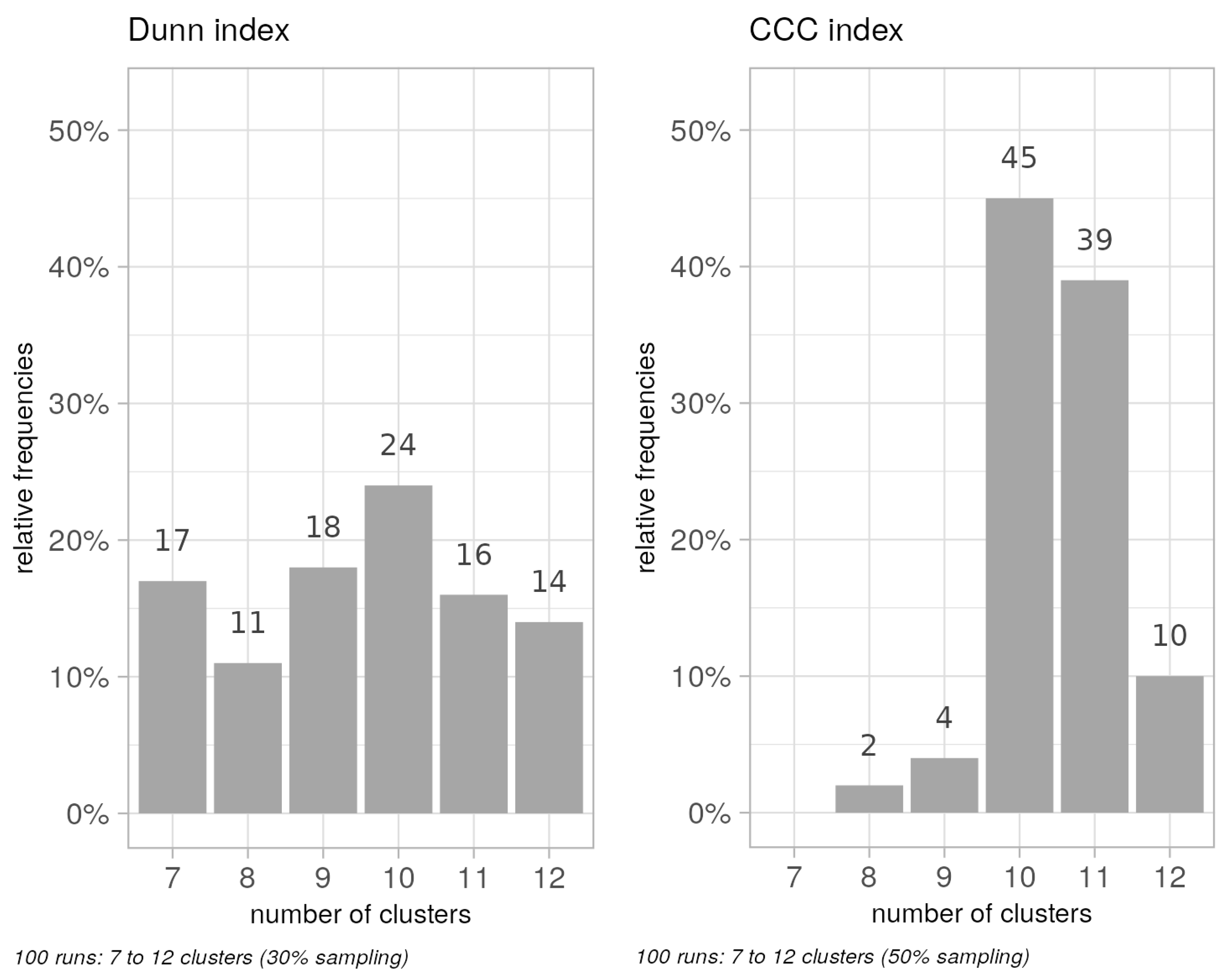
All 18 selected raster datasets of Table 1 were harmonized in a common spatial resolution of 1 ha analysis cell, following resampling procedures (bilinear interpolation). Feature scaling through standardization was carried out in order to establish a common scale of variance throughout the input data (i.e., a mean of zero and a standard deviation of one for all variables). In order to estimate the optimal number of clusters for k-means, the Dunn and CCC indices were repeatedly evaluated for the different possible numbers of clusters in the R-environment using the package “NbClust” [36]. The computational cost of the process was a critical factor, depending both on the size of the dataset (69.7 K records × 18 variables) and on the number of possible clusters examined at each repetition. Both indices were processed individually in 100 group repetitions of the k-means algorithm with 6 possible numbers of clusters, i.e., from 7 up to 12. The range of the possible number of clusters was introduced in order to reduce the computational burden of the process on a realistic basis of the expected number of terroir units. For computational efficiency, a total of 1200 indices (600 each index) were computed on a subset of the initial data population, using the 18 variables of Table 1 and repetitive k-means with random initialization. Dunn indices were evaluated on 30% sampling from the initial data population; CCC, being computationally more efficient, were evaluated on 50% sampling accordingly.
The resulting optimal numbers of clusters for each index are presented in the form of their frequency distribution (Figure 2). Both Dunn and CCC indices suggest the number of 10 as the most frequent optimal number of clusters, although most possible numbers from 7 to 12 have emerged as optimal with lower frequencies. Following this suggested number of clusters, k-means clustering was computed on the 18 variables of Table 1, using Hartigan and Wong algorithm’s implementation in base-R [37].

3.1. Cluster Stability

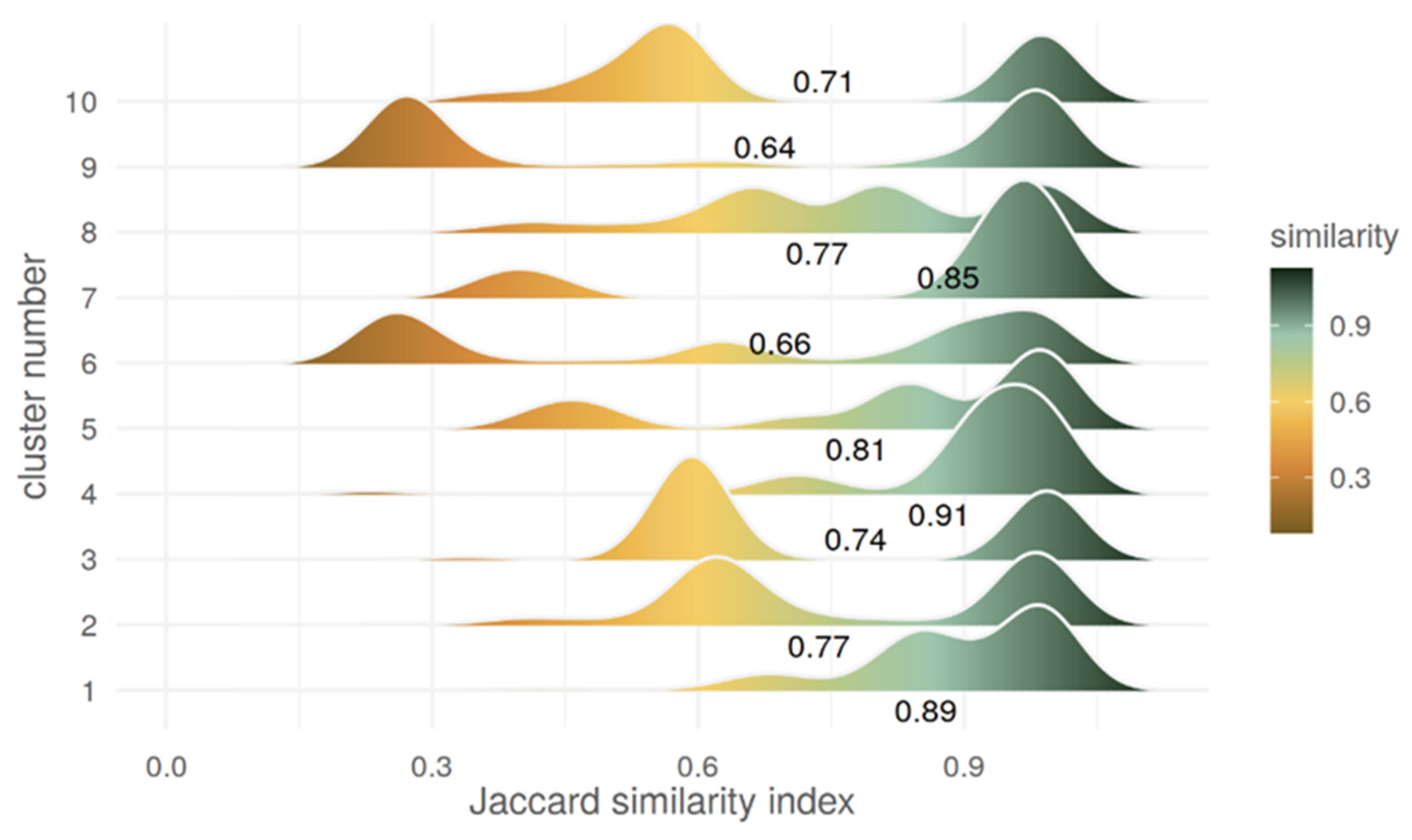
Stability analysis for the 10-cluster k-means result was carried out with bootstrap repetitions using package “fpc” in R-environment [38]. The distributions of similarity metrics (i.e., Jacard similarity index) were plotted for every cluster in parallel density plots as a ridge plot (Figure 3). The mean Jaccard index displayed for each cluster was an indication of each cluster’s stability.
The Dunn and CCC index suggestion of 10 clusters was realistic as all clusters were stable (Figure 3), with 8 out of 10 clusters scoring 0.71–0.91 and two clusters scoring 0.64 and 0.66 stability index. Concerning the two clusters, No.9 and No.6, although they turned out stable according to the criterion of mean stability index, it is apparent from their Jaccard index distribution that a substantial number of repetitions yielded low-stability values. This unstable performance is related to the extreme variability, inherent in specific input features for each cluster explicitly. In particular, cluster No.6 is scattered across various hillsides surrounding the plain of Drama, while cluster No.9 is at the downstream part of the plain of Drama, where various alluvial deposits have contributed to high soil variability. The extent of variability in relation to the mean for each population (CV %) reaches the global maximum inside cluster No.6 for most (five out of nine) of the climatic variables (GSTmax 115%, GSTmin 113%, GSpET 126%, GSwv 135%, WINpr 108%), while also exhibiting extreme values for soil and topographic variables (Clay 116%, BD 117%, Aspect 117%). Similarly, inside cluster No.9, variability reaches a global maximum for the soil fraction of Clay (136%), while also exhibiting extreme values for Aspect (128%), CEC (100%), and WINpr (106%).
By deviating from the suggested optimal number of 10 clusters, alternate clustering solutions using k-means with the Hartigan and Wong algorithm were generated and subsequently checked for stability by bootstrap repetitions of the Jaccard similarity index. Any additional decrease or increase in the desired number of clusters in k-means deteriorated the overall stability of the resulting clusters further (results not shown). Consequently, the k-means 10-cluster solution was considered as optimal to receive a physical interpretation toward the understanding of the drivers of terroir.

3.2. NTUs Distribution and Characterization

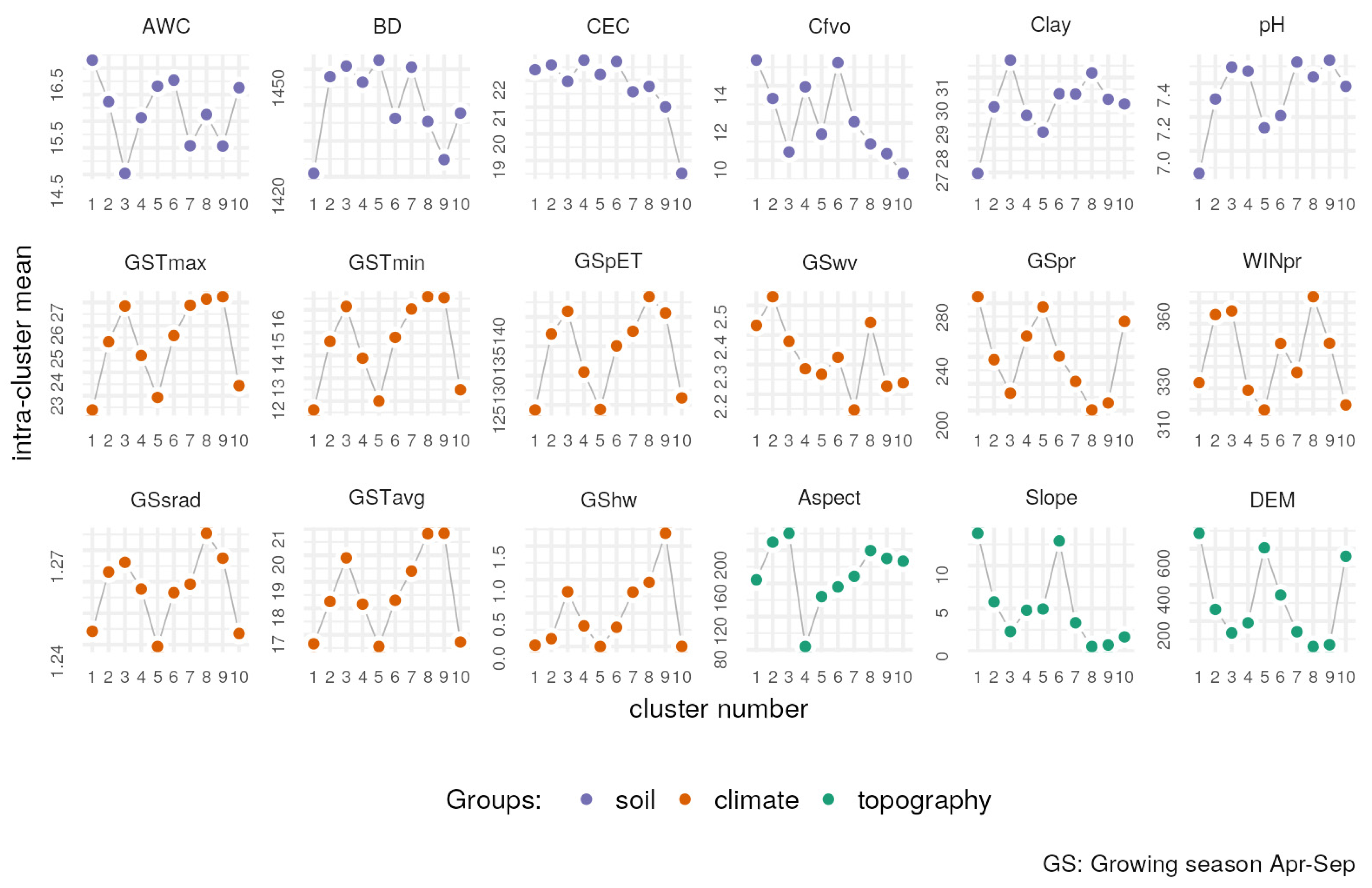
The resulting clustering solution of 10 clusters representing the NTUs of Drama Regional Unit is presented in Figure 4, and the intra-cluster means for every input variable are presented in Figure 5.
Clustering revealed 10 NTUs, which are, for the most part, located in distinct areas and can be grouped into three sub-regions (Figure 4 and Figure 5). As anticipated, topography had a profound impact on the spatial distribution of climatic characteristics of the Drama region. NTUs 1, 5, and 10 are generally distributed in the northwestern part of the Drama region with the highest elevation (500–700 m); NTUs 2 and 6 were mostly located in the second highest elevation zone (200–500 m) in the central-eastern part of Drama region, while NTUs 3, 4, 7, 8, and 9 occupy the lowest elevation zone (up to 200 m) and are distributed across the whole southern part of Drama region, where most of the current viticultural areas occur.
Growing season minimum, maximum, mean temperatures, evapotranspiration, and precipitation were affected by variations in altitude at different scales. Northwestern NTUs (1, 5, and 10) are generally characterized by homogeneous climatic features. These terroir units present the lowest temperatures (minimum ≈ 12 °C, maximum ≈ 23 °C, mean ≈ 17 °C) and the highest growing season precipitation rates (≈280 mm) on average, coupled with evapotranspiration of ≈125 mm. Northeastern NTUs 2 and 6, situated at the intermediate altitude clusters, presented higher growing season temperatures (minimum ≈ 15 °C, maximum ≈ 26 °C, mean ≈ 18.5 °C) and a precipitation/evapotranspiration ratio ≈ 250/140 mm. NTUs 3, 8, and 9, which constitute the southeast part of the Drama region, exhibited the highest values of growing season temperatures (minimum ≈ 17 °C, maximum ≈ 27 °C, mean ≈ 21 °C) and minimum precipitation (≈200 mm), coupled with evapotranspiration of ≈150 mm. NTU 9 presented the overall warmer climate with the highest heat occurrence frequency (≈2%), closely followed by NTU 8. However, as we move toward the eastern part corresponding to the narrow valley between Mounts Menikion and Falakro (NTUs 7 and mainly 4), temperature conditions become cooler, which suggests a further climatic division of the southern sub-region. NTU 8 is additionally characterized by a winter precipitation maximum (≈370 mm).
In terms of topography, apart from the differences in elevation, the resulting NTUs are further differentiated by their average slope and aspect. NTUs 1 and 6 are the only ones characterized by steep slopes (reaching 15%). Among the rest, NTUs 8 and 9 (in the low-altitude southern sub-region) and 10 (in the high-altitude northwest sub-region) are practically on flat terrain, with the remaining ones presenting an average slope of 3 to 6%. Interestingly, apart from the NE exposure of NTU 4 situated mostly on the slopes of Menikion mountain, all clusters share a prevailing S (NTUs 1, 5, 6, and 7) to SW (2, 3, 8, 9, and 10) slope aspect.
The variability of soil properties is mainly responsible for the local terroir distribution. Although cluster separation is strongly influenced by the short-range variation of soil properties, mainly pedological characteristics, i.e., pH, AWC, clay fraction, and coarse fragments fraction, actual soil features varied little among NTUs. Soils were generally rich (C.E.C. ranged between 16 and 27 meq/100 g, Table 1) with a good porosity (soil bulk density < 1.5 g/cm3) and a fraction of coarse element >10%. Its pH ranged between 6.9 and 7.5.
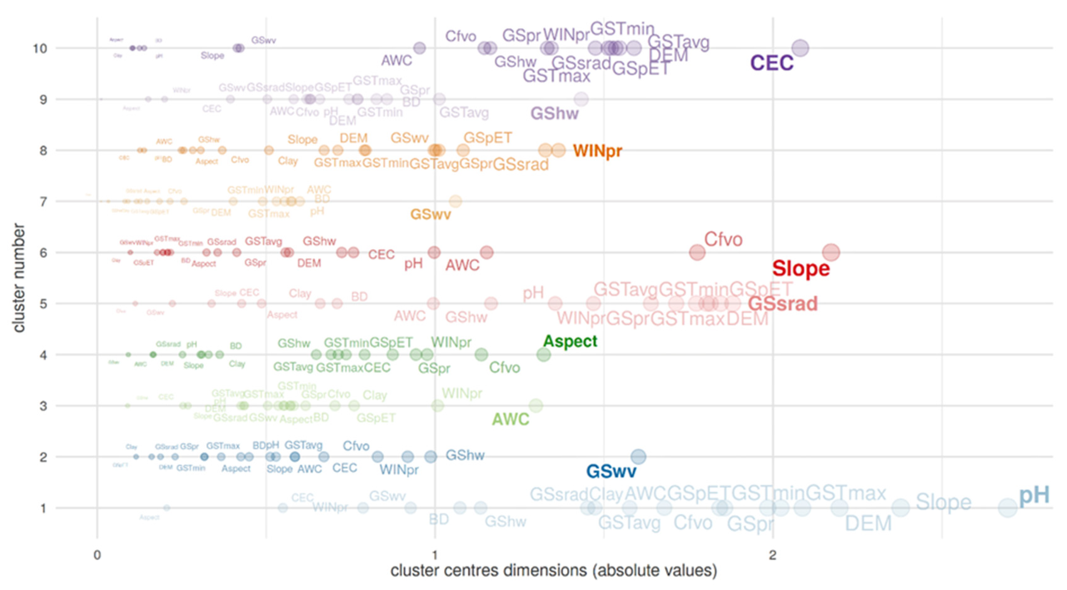
Focusing on cluster centroids and their dimensions in feature space, the Euclidean distances that represent the magnitude of feature dimensions are plotted along the X-axis in Figure 6 for every cluster. The largest absolute feature dimension per cluster centroid was highlighted in order to assist the characterization of the derived clusters and the physical description of the NTUs that is carried out using the intra-cluster means for every input feature of Figure 5.
NTU1 covers a total area of 3160 ha, scattered across the entire northern part of the region in high-altitude areas, exhibiting considerable terrain variability under soils that appear at the lowest end of the pH scale. The pH, Slope, and DEM are highly important features for the delineation of the terroir unit. NTU2 is situated mainly in the eastern part of the region, covering 5369 ha of the hilly landscape of agricultural areas from south to northeast, where wind velocity exhibits its global maximum. Naturally, GSwv, i.e., wind velocity during the growing season, has a high influence on its delineation. NTU3, which is adjacent to NTU2, continues to the southern parts of the eastern region, occupying an area of 6888 ha, exhibiting the lowest AWC of the entire agricultural region, heavily influencing the terroir unit’s delineation. NTU4 covers an area of 4085 ha in the central–western part of the region, where its distinctive exposure and soil coarse fragment volume percentage have highly influenced its delineation. NTU5 is scattered in areas of high altitude in the northwestern part of the region, delineated under the impact of almost all the climatic variables, accumulating an area coverage of 5520 ha. NTU6 covers an area of 2942 ha which is the minimum area coverage among the terroir units identified. Scattered across the hilly landscape surrounding the plain of Drama, its delineation is heavily influenced by the slope percentage of topographic variation and by the soil coarse fragment volume percentage. NTU7 is one of the largest terroir units, with an area coverage of 13,008 ha. Situated in the central–eastern part of the Drama region, its delineation is influenced by soil characteristics, such as AWC, pH, and BD, and mostly by the global minima of wind velocity (GSwv) during the growing season. NTU8 is mostly located in the southern part of the region, occupying an area of 8908 ha. Its delineation is influenced by almost all the climatic variables, mostly by the precipitation during the winter season (WINpr). NTU9, situated in the southern part of the region, adjacent to NTUs 8, 7, and 3, is the largest terroir unit identified in the region, with an area coverage of 15,008 ha. Influenced by both soil and climatic variables, its delineation is heavily impacted by the global maximum of heat-wave occurrence that appears as a hot spot in the area occupied by this unit. NTU10 occupies the northwestern plateau of Kato Nevrokopi, covering an area of 4836 ha. Its delineation is influenced by most of the climatic variables and elevation but mostly by the lower CEC that characterizes the loamy and sandy–loamy soils of the area.

3.3. External Validation

External validation of the derived NTUs was performed by testing the variance of the observed vine response (NDVI) against the proposed terroir zonation. A time series of Sentinel-2 NDVI data at 10 m spatial resolution, covering the growth period from April to September, was extracted on a median cell basis to the polygons of the established vineyards scattered across the NTUs. Vineyards were distributed among all the NTUs (Figure 7), with the exception of NTU10, which is the northwestern plateau of Kato Nevrokopi. This area has not been used for viticultural purposes yet but was included in terroir zonation as a potential NTU, capable of supporting viticultural activities in the future. Thus, NTU10 was excluded from further validation due to the absence of vineyard data. The extracted data set consisted of 5545 NDVI measurements among nine different NTUs.
Evaluation of the relevance of the derived NTUs based on vine NDVI was performed through a one-way analysis of variance. Variance homogeneity was tested prior to analysis using Levene’s test [39]. Homoscedasticity was not met since the variances were found to be significantly different. Alternatively, in the absence of homogeneity of variances, Welch ANOVA was adopted [40]. The initial results showed significant differences among the derived NTUs (DFd = 121.5, statistic = 21.4, p ≤ 0.0001). The presence of spatial autocorrelation in the response variable’s (NDVI) residuals that were evident (Moran’s I = 0.65, p ≤ 0.0001) compromised the above result because it violated the assumption of stochastic independence among observations, on which statistical inference is based. Overlooking this issue could potentially lead to biased standard errors and/or biased parameter estimates, as well as artificially inflated degrees of freedom. Thus, we applied semiparametric filtering of spatial dependence, using simultaneous autoregressive (SAR) spatial models, implemented in package “spatialreg” in R-environment, resulting in spatially uncorrelated NDVI residuals (Moran’s I = −0.08, p = 0.46) [41,42]. Welch test confirmed the significant differences among the NTUs (DFd = 132.4, statistic = 47.7, p ≤ 0.0001), i.e., the between-cluster variability of NDVI is significantly higher compared to the within-cluster variability.
The mean NDVI from Sentinel-2 during the growth period was plotted per NTU and grape variety (Figure 7). Sauvignon blanc is absent only from NTU9 and generally presents the higher canopy growth in NTUs 5 and 6 with the higher AWC (Figure 5), where it represents the total area of vineyards. Sauvignon blanc is a variety cultivated to produce wines with green/unripe aromas, which are maximized in soils with high water and nitrogen content. These soils lead to denser canopies reducing light penetration to the fruiting zone of the vines. Thus, NDVI values of Sauvignon blanc vineyards are relatively high in all NTUs, except for the NTU1 with the steeper slope and highest amount of course elements in the soil. The second most important white variety of the area, Assyrtiko, a medium vigor variety, presents lower NDVI in all NTUs. Among the red varieties, although Agiorgitiko is considered more vigorous than Merlot and Cabernet Sauvignon, it presents on average lower NDVI values than Cabernet Sauvignon and Merlot, but no clear differences were observed either between varieties or between NTUs within the same variety. It has been previously shown that NDVI has certain limitations, mostly related to the interference of different vineyard management practices used between locations, cultivars, or growers, which can significantly reduce NDVI credibility in the delineation of management zones in vineyards [43].

3.4. Implications of NTUs in Vini-Viticulture

A major outcome of terroir studies is assisting in the selection of the right grape variety with respect to the soil and climate in order to maximize the expression of terroir at specific locations [16,44]. Thus, the assessment of the compiled clustering results can be helpful in highlighting the most suitable NTUs for each major grape variety in the Drama region.
The temperature regime during grape ripening is of major importance in aroma type in wine and is expected to be of high influence in most of the derived NTUs. Temperature modulates the biosynthesis of the grape aroma precursors and also their breakdown rate, with different requirements between volatile chemical groups. For example, cooler regions are associated with increased expression of vegetative aromas [45]. On the contrary, for red grapes, for which more fruity aromas are desirable, warmer climates with higher temperatures are more suitable [46]. Grape exposure to sunlight also exerts a significant role on the metabolic pathway of grape aroma-related compounds, stimulating the production of those associated with floral and fruity characteristics while, conversely, decreasing those related to vegetative or spicy ones [47,48].
Terroir’s effect on wine flavor is also reported to be linked to water and nutrient availability. Bramley, Ouzman, and Trought [6] accomplished terroir zoning on the basis of identifying the strong impact of topographic variation on both soil hydrology and soil fertility. Vine water status is also influenced by meteorological factors, such as rainfall and reference evapotranspiration [44]. Grape metabolites responsible for the fruity wine aromas are maximized under conditions of moderate water and nutrient availability, while those related to the more vegetative ones are more expressed under higher nitrogen and water reserves [49]. As a result, winegrape cultivars respond differently to water conditions depending on the prevailing volatile compounds responsible for their ‘varietal’ character and their vocation for certain styles of wines.
Sauvignon blanc, a French cultivar known for producing “green” aromas, is the most widely planted white variety in the Drama region. It has been previously shown that a sustained water deficit limits Sauvignon blanc aroma potential [49]. Water deficit is also reported to decrease the levels of compounds responsible for vegetative aromas (methoxypyrazines), which are desirable in white wines from this variety [50]. Moreover, its cultivation in cool sites can lead to less tropical fruit, and more boxwood-like aromas in wines are generally considered the most “typical” for Sauvignon blanc wines. However, for Assyrtiko, the second most important white variety of the Drama region originating from Santorini island, moderate to high water deficits are more suitable for the expression of its flagship “mineral” aromatic character. Similarly, the aromatic quality of red grapes and wines from the varieties Agiorgitiko and Cabernet Sauvignon is achieved under more stressful water conditions [51,52].
In cooler conditions and/or higher water availability conditions (NTUs of the northern part of the Drama region), Sauvignon blanc grapes would be expected to achieve better aromatic ripeness. Slope percentage and orientation (aspect), though, could allow for a fine-tuning of variety selection within sub-regions as south-facing slopes in the Northern Hemisphere are generally warmer. However, the aspect contributing to the terroir effect is more pronounced with increasing slope, i.e., in the case of cooler climate NTUs 1 and 6, their S slope orientation may alleviate some of the climatic restrictions regarding the adaptation of late ripening varieties related to elevation (especially for NTU 1).
Based on these considerations, within the two northern sub-regions, the coolest northwest NTUs 5 and 10 should favor more “vegetative”-style wines, while NTU 1, characterized by steep slopes facing south (e.g., possibly more limiting water conditions and higher sun exposure), could be more suitable for concentrated white wines. Similarly, between the northeast NTUs situated in the intermediate elevation and climate zone, NTU 2 would be more suited for Sauvignon blanc, while NTU 6, characterized by higher slopes of southern exposure, would be more adapted to the cultivation of early-ripening red varieties, such as Merlot [53]. In these areas, the cultivation of red and late ripening varieties would require the reduction of yields, the use of rootstocks of the shorter vegetative growth cycle, and other vineyard adaptations by the growers to allow a better ripening.
Warmer locations of the lowest elevation zone should be avoided for Sauvignon blanc, with the exception of NTU 4. Narrow valleys are often associated with cool valley floor temperatures due to the downhill movement of the heavier cool air masses. In addition, the mean slope of NTU 4, although not high (approximately 5% on average), must be taken into consideration since it is the only one among the warmer low-elevation areas of the southern sub-region with a north aspect, a feature that can significantly alter its microclimate compared to the rest of the NTUs of this sub-region, with positive consequences regarding its suitability to grow early ripening varieties, such as Sauvignon blanc and Merlot. The warmer NTUs 7 and 3 of the southern part of the region would be suited to either Assyrtiko or late red varieties, such as Agiorgitiko and Cabernet Sauvignon. However, Sauvignon blanc forms a significant part of the cultivated surface under vines in those NTUs. In those areas, a more severe intervention by the vineyard managers will be needed in terms of canopy management, rational use of irrigation and fertilization, and soil management to improve grapevine performance, even though this would mask the terroir effect.
Finally, the very warm NTUs 8 and 9, on flat soils, are generally the least suitable for quality wines. Sauvignon blanc is scarce or completely absent from these areas, while red varieties and late-ripening ones (i.e., Cabernet Sauvignon, Agiorgitiko, and Assyrtiko) are cultivated. In the frame of current and future global warming, those areas would be either excluded from the demarcated areas of Geographical Indication wines or adopt more prescriptive legislation for recommended varieties and wine styles per NTU.
This article presents a new approach to terroir studies through a new zoning methodology, with the aim to provide useful directions to the expanding wineries of the region and also to contribute to terroir resilience to climate change. Protected Designation Areas (PDO—Protected Designation of Origin or PGI—Protected Geographical Indication) will be most likely threatened by climate change in the future, mostly by challenging their ability to produce wines that will continue to reflect their geographical origin and meet consumer expectations. The resilience of the wine industry will, therefore, depend on the adaptation policies in the viticultural and enological processes. In this view, the results of this work offer a powerful tool for the whole wine sector to successfully define the precise adaptation strategies to preserve the “expression” of terroir, such as (1) rearrangement of PDO areas boundaries, (2) optimization of variety distribution within the PDO areas, (3) modification of vineyard decisions, such as choice of rootstocks, clones, training systems, or (4) identification of new suitable land for viticulture.

3.5. Advantages and Limitations of the Proposed Methodology

The spatial modeling of NTUs includes the acquisition and processing of a large array of geospatial information regarding the three most important environmental factors that make up the terroir effect on different scales. Since the issue of scale is inherent in any characterization of terroir, the spatial level of analysis of each NTU should be studied further, taking into account the concept of viticultural validation. The hierarchy of the terroir variables’ effects may vary according to the scale. The climate, in combination with grapevine variety, is perhaps the most important component of the terroir influence at the regional level. Sub-regionally, geomorphology and related topo-climatic effects might be the driving factors that are able to explain differences in vine development and grape composition. Locally, the terroir effect is governed by the spatial distribution of pedological soil properties, i.e., clay fraction, coarse fragments, and bulk density, which greatly affect soil hydrology (AWC).
Cluster analysis is ideal for the multi-variate nature of viticultural terroir spatial modeling. Still, it is important to note that cluster analysis is of exploratory nature, and the output of clustering only suggests hypotheses. While several clustering methods have been published, and more are constantly being developed, no one clustering algorithm has been demonstrated to be superior to other algorithms in the terroir modeling application space. K-means’ major constraint is that the outcome of clustering strongly depends on the process initialization, which can be addressed to an extent by better initialization techniques and repetitive k-means.

4. Conclusions

Based on public-access geospatial information from online sources regarding soil, climate, and topography of the wine-production environment, we established a data-driven approach toward terroir zoning and NTUs identification, which was demonstrated in the Drama region (Greece). The optimum number of clusters (n = 10) was identified by the Dunn index and CCC computations and performed by k-means clustering using the Hartigan and Wong algorithm. The clustering solution was proven stable by bootstrap repetitions of the Jaccard similarity index, while all deviations around the suggested number of clusters yielded unstable solutions. Therefore, the 10-cluster k-means solution is optimal in the sense that it exhibits sufficient overall stability in order to receive a meaningful description toward a true understanding of the drivers of terroir. The practical value of the proposed methodology lies in the fact that it provides the wine-makers the necessary tool to make unbiased, i.e., data-driven decisions regarding the distribution of appropriate plant material (varieties) across the varying landscape of environmental factors based on the established terroir zonation.
Spatial modeling of viticultural terroir lays the foundation to address major environmental challenges in the forthcoming years, such as terroir sustainability and efficient implementation of appropriate management strategies at multiple spatial scales. Such strategies, by taking into account the potential impact of climate change in viticulture and considering the narrow climatic range for optimum quality and production that individual wine-grape varieties exhibit, can provide proper mitigation measures (e.g., management practices or plant relocation) based on the established terroir zonation. Overall, terroir modeling is highly possible to be viewed as part of the concept of ecosystem services, such as agricultural ecosystems for viticulture, whose services need to be assessed and updated on an ongoing basis.

Author Contributions

Conceptualization, T.K.A. and S.K.; methodology, N.K. and T.K.A.; software, N.K.; validation, N.K., S.T. and S.K.; formal analysis, N.K. and T.K.A.; data curation, N.K. and G.B.; writing—original draft preparation, N.K., T.K.A. and S.K.; writing—review and editing, all authors; visualization, N.K.; supervision, T.K.A. and S.K.; funding acquisition, S.K. All authors have read and agreed to the published version of the manuscript.

Funding

This research was co-financed by the European Regional Development Fund of the European Union and Greek national funds through the Operational Program Competitiveness, Entrepreneurship, and Innovation, under the call RESEARCH—CREATE—INNOVATE (project code: Τ2ΕΔΚ-02974).

Institutional Review Board Statement

Not applicable.

Data Availability Statement

Publicly available datasets were analyzed in this study. This data can be found at the respective sources mentioned in the manuscript.

Conflicts of Interest

The authors declare no conflict of interest.

References

  1. Carey, V.A. Spatial Characterisation of Natural Terroir Units for Viticulture in the Bottelaryberg-Simonsberg-Helderberg Winegrowing Area; Stellenbosch University: Stellenbosch, South Africa, 2001. [Google Scholar]
  2. Bodin, F.; Morlat, R. Characterization of viticultural terroirs using a simple field model based on soil depth I. Validation of the water supply regime, phenology and vine vigour, in the Anjou vineyard (France). Plant Soil 2006, 281, 37–54. [Google Scholar] [CrossRef]
  3. Tesic, D.; Woolley, D.J.; Hewett, E.W.; Martin, D.J. Environmental effects on cv. Cabernet Sauvignon (Vitis vinifera L.) grown in Hawke’s Bay, New Zealand.: 1. Phenology and characterisation of viticultural environments. Aust. J. Grape Wine Res. 2002, 8, 15–26. [Google Scholar] [CrossRef]
  4. Van Leeuwen, C.; Friant, P.; Choné, X.; Tregoat, O.; Koundouras, S.; Dubourdieu, D. Influence of Climate, Soil, and Cultivar on Terroir. Am. J. Enol. Vitic. 2004, 55, 207–217. [Google Scholar] [CrossRef]
  5. Priori, S.; Barbetti, R.; L’Abate, G.; Bucelli, P.; Storchi, P.; Costantini, E.A. Natural terroir units, Siena province, Tuscany. J. Map. 2014, 10, 466–477. [Google Scholar] [CrossRef] [Green Version]
  6. Bramley, R.G.; Ouzman, J.; Trought, M.C. Making sense of a sense of place: Precision viticulture approaches to the analysis of terroir at different scales. OENO One 2020, 54, 903–917. [Google Scholar] [CrossRef]
  7. Vaudour, E.; Costantini, E.; Jones, G.V.; Mocali, S. An overview of the recent approaches to terroir functional modelling, footprinting and zoning. Soil 2015, 1, 287–312. [Google Scholar] [CrossRef] [Green Version]
  8. Mackenzie, D.; Christy, A. The role of soil chemistry in wine grape quality and sustainable soil management in vineyards. Water Sci. Technol. 2005, 51, 27–37. [Google Scholar] [CrossRef] [PubMed]
  9. Fraga, H.; Malheiro, A.C.; Moutinho-Pereira, J.; Cardoso, R.M.; Soares, P.M.; Cancela, J.J.; Pinto, J.G.; Santos, J.A. Integrated analysis of climate, soil, topography and vegetative growth in Iberian viticultural regions. PLoS ONE 2014, 9, e108078. [Google Scholar] [CrossRef]
  10. Flexas, J.; Galmés, J.; Gallé, A.; Gulías, J.; Pou, A.; Ribas-Carbo, M.; Tomàs, M.; Medrano, H. Improving water use efficiency in grapevines: Potential physiological targets for biotechnological improvement. Aust. J. Grape Wine Res. 2010, 16, 106–121. [Google Scholar] [CrossRef]
  11. Jones, G.; Snead, N.; Nelson, P. Geology and wine 8. Modeling viticultural landscapes: A GIS analysis of the terroir potential in the Umpqua Valley of Oregon. Geosci. Can. 2004, 31, 167–178. [Google Scholar]
  12. Jones, G.V.; Davis, R.E. Climate influences on grapevine phenology, grape composition, and wine production and quality for Bordeaux, France. Am. J. Enol. Vitic. 2000, 51, 249–261. [Google Scholar] [CrossRef]
  13. Santos, J.A.; Malheiro, A.C.; Karremann, M.K.; Pinto, J.G. Statistical modelling of grapevine yield in the Port Wine region under present and future climate conditions. Int. J. Biometeorol. 2011, 55, 119–131. [Google Scholar] [CrossRef]
  14. Jones, G.V. Climate and terroir: Impacts of climate variability and change on wine. Geosci. Can. Repr. Ser. 2006, 9, 203–217. [Google Scholar]
  15. Zsófi, Z.; Tóth, E.; Rusjan, D.; Bálo, B. Terroir aspects of grape quality in a cool climate wine region: Relationship between water deficit, vegetative growth and berry sugar concentration. Sci. Hortic. 2011, 127, 494–499. [Google Scholar] [CrossRef]
  16. Van Leeuwen, C.; Barbe, J.-C.; Darriet, P.; Geffroy, O.; Gomès, E.; Guillaumie, S.; Helwi, P.; Laboyrie, J.; Lytra, G.; Le Menn, N.; et al. Recent advancements in understanding the terroir effect on aromas in grapes and wines. OENO One 2020, 54, 985–1006. [Google Scholar] [CrossRef]
  17. Costantini, E.A.C.; Bucelli, P. Soil and terroir. In Soil Security for Ecosystem Management; Springer International Publishing: Cham, Switzerland, 2014; pp. 97–133. [Google Scholar]
  18. Vaudour, E. The Quality of Grapes and Wine in Relation to Geography: Notions of Terroir at Various Scales. J. Wine Res. 2002, 13, 117–141. [Google Scholar] [CrossRef]
  19. Lagacherie, P.; Bailly, J.-S.; Monestiez, P.; Gomez, C. Using scattered hyperspectral imagery data to map the soil properties of a region. Eur. J. Soil Sci. 2012, 63, 110–119. [Google Scholar] [CrossRef] [Green Version]
  20. Morari, F.; Castrignanò, A.; Pagliarin, C. Application of multivariate geostatistics in delineating management zones within a gravelly vineyard using geo-electrical sensors. Comput. Electron. Agric. 2009, 68, 97–107. [Google Scholar] [CrossRef]
  21. Castrignanò, A.; Costantini, E.A.; Barbetti, R.; Sollitto, D. Accounting for extensive topographic and pedologic secondary information to improve soil mapping. Catena 2009, 77, 28–38. [Google Scholar] [CrossRef]
  22. Hengl, T.; Mendes de Jesus, J.; Heuvelink, G.B.; Ruiperez Gonzalez, M.; Kilibarda, M.; Blagotić, A.; Shangguan, W.; Wright, M.N.; Geng, X.; Bauer-Marschallinger, B. SoilGrids250m: Global gridded soil information based on machine learning. PLoS ONE 2017, 12, e0169748. [Google Scholar] [CrossRef] [PubMed] [Green Version]
  23. Tóth, B.; Weynants, M.; Pásztor, L.; Hengl, T. 3D soil hydraulic database of Europe at 250 m resolution. Hydrol. Process. 2017, 31, 2662–2666. [Google Scholar] [CrossRef] [Green Version]
  24. Hartigan, J.A.; Wong, M.A. Algorithm AS 136: A k-means clustering algorithm. J. R. Stat. Soc. Ser. C 1979, 28, 100–108. [Google Scholar] [CrossRef]
  25. Morissette, L.; Chartier, S. The k-means clustering technique: General considerations and implementation in Mathematica. Tutor. Quant Methods Psychol. 2013, 9, 15–24. [Google Scholar] [CrossRef] [Green Version]
  26. Fränti, P.; Sieranoja, S. How much can k-means be improved by using better initialization and repeats? Pattern Recognit. 2019, 93, 95–112. [Google Scholar] [CrossRef]
  27. Jain, A.K. Data clustering: 50 years beyond K-means. Pattern Recog. Lett. 2010, 31, 651–666. [Google Scholar] [CrossRef]
  28. Äyrämö, S.; Kärkkäinen, T. Introduction to partitioning-based clustering methods with a robust example. In Reports of the Department of Mathematical Information Technology. Series C, Software Engineering and Computational Intelligence; National Library of Finland: Helsinki, Finland, 2006. [Google Scholar]
  29. Dunn, J.C. Well-separated clusters and optimal fuzzy partitions. J. Cybern. 1974, 4, 95–104. [Google Scholar] [CrossRef]
  30. Sarle, W.S. SAS Technical Report A-108, Cubic Clustering Criterion; SAS Institute Inc: Cary, NC, USA, 1983; p. 56. [Google Scholar]
  31. Brun, M.; Sima, C.; Hua, J.; Lowey, J.; Carroll, B.; Suh, E.; Dougherty, E.R. Model-based evaluation of clustering validation measures. Pattern Recognit. 2007, 40, 807–824. [Google Scholar] [CrossRef]
  32. Hennig, C. Cluster-wise assessment of cluster stability. Comput. Stat. Data Anal. 2007, 52, 258–271. [Google Scholar] [CrossRef] [Green Version]
  33. Santesteban, L.; Guillaume, S.; Royo, J.; Tisseyre, B. Are precision agriculture tools and methods relevant at the whole-vineyard scale? Precis. Agric. 2013, 14, 2–17. [Google Scholar] [CrossRef] [Green Version]
  34. Fiorillo, E.; Crisci, A.; De Filippis, T.; Di Gennaro, S.; Di Blasi, S.; Matese, A.; Primicerio, J.; Vaccari, F.; Genesio, L. Airborne high-resolution images for grape classification: Changes in correlation between technological and late maturity in a Sangiovese vineyard in Central Italy. Aust. J. Grape Wine Res. 2012, 18, 80–90. [Google Scholar] [CrossRef]
  35. Lamb, D.W.; Weedon, M.; Bramley, R. Using remote sensing to predict grape phenolics and colour at harvest in a Cabernet Sauvignon vineyard: Timing observations against vine phenology and optimising image resolution. Aust. J. Grape Wine Res. 2004, 10, 46–54. [Google Scholar] [CrossRef] [Green Version]
  36. Charrad, M.; Ghazzali, N.; Boiteau, V.; Niknafs, A. NbClust: An R package for determining the relevant number of clusters in a data set. J. Stat. Softw. 2014, 61, 1–36. [Google Scholar] [CrossRef] [Green Version]
  37. Team, R.C. R: A Language and Environment for Statistical Computing; R Foundation for Statistical Computing: Vienna, Austria. Available online: http://www.R-project.org/ (accessed on 5 January 2023).
  38. Hennig, C. ‘fpc: Flexible Procedures for Clustering’, R-Package Version 2.2-9. Available online: https://cran.r-project.org/web/packages/fpc/ (accessed on 30 November 2022).
  39. Levene, H. Robust tests for equality of variances. In Contributions to Probability and Statistics: Essays in Honor of Harold Hotelling; Olkin, I., Hotelling, H., Eds.; Stanford University Press: Redwood City, CA, USA, 1960; pp. 278–292. [Google Scholar]
  40. Welch, B.L. On the comparison of several mean values: An alternative approach. Biometrika 1951, 38, 330–336. [Google Scholar] [CrossRef]
  41. Tiefelsdorf, M.; Griffith, D.A. Semiparametric filtering of spatial autocorrelation: The eigenvector approach. Environ. Plan. A 2007, 39, 1193–1221. [Google Scholar] [CrossRef]
  42. Bivand, R.; Millo, G.; Piras, G. A review of software for spatial econometrics in R. Mathematics 2021, 9, 1276. [Google Scholar] [CrossRef]
  43. Anastasiou, E.; Balafoutis, A.; Theocharis, S.; Theodorou, N.; Koundouras, S.; Fountas, S. Assessment of Laser Scanner Use under Different Settings in Two Differently Managed Vineyards for Estimating Pruning Wood Parameters. AgriEngineering 2022, 4, 47. [Google Scholar] [CrossRef]
  44. Van Leeuwen, C.; Trégoat, O.; Choné, X.; Bois, B.; Pernet, D.; Gaudillère, J.-P. Vine water status is a key factor in grape ripening and vintage quality for red Bordeaux wine. How can it be assessed for vineyard management purposes? OENO One 2009, 43, 121–134. [Google Scholar] [CrossRef]
  45. Allen, M.S.; Lacey, M.J.; Harris, R.L.N.; Brown, W.V. Contribution of Methoxypyrazines to Sauvignon blanc Wine Aroma. Am. J. Enol. Vitic. 1991, 42, 109–112. [Google Scholar] [CrossRef]
  46. Zhang, P.; Howell, K.; Krstic, M.; Herderich, M.; Barlow, E.W.; Fuentes, S. Environmental Factors and Seasonality Affect the Concentration of Rotundone in Vitis vinifera L. cv. Shiraz Wine. PLoS ONE 2015, 10, e0133137. [Google Scholar] [CrossRef] [Green Version]
  47. Bureau, S.M.; Baumes, R.L.; Razungles, A.J. Effects of Vine or Bunch Shading on the Glycosylated Flavor Precursors in Grapes of Vitis vinifera L. Cv. Syrah. J. Agric. Food Chem. 2000, 48, 1290–1297. [Google Scholar] [CrossRef] [PubMed]
  48. Marais, J. Sauvignon blanc cultivar aroma—A review. South Afr. J. Enol. Vitic. 1994, 15, 41–45. [Google Scholar] [CrossRef] [Green Version]
  49. Des Gachons, C.P.; Leeuwen, C.V.; Tominaga, T.; Soyer, J.-P.; Gaudillère, J.-P.; Dubourdieu, D. Influence of water and nitrogen deficit on fruit ripening and aroma potential of Vitis vinifera L cv Sauvignon blanc in field conditions. J. Sci. Food Agric. 2005, 85, 73–85. [Google Scholar] [CrossRef]
  50. Sala, C.; Busto, O.; Guasch, J.; Zamora, F. Contents of 3-alkyl-2-methoxypyrazines in musts and wines from Vitis vinifera variety Cabernet Sauvignon: Influence of irrigation and plantation density. J. Sci. Food Agric. 2005, 85, 1131–1136. [Google Scholar] [CrossRef]
  51. Koundouras, S.; Hatzidimitriou, E.; Karamolegkou, M.; Dimopoulou, E.; Kallithraka, S.; Tsialtas, J.T.; Zioziou, E.; Nikolaou, N.; Kotseridis, Y. Irrigation and Rootstock Effects on the Phenolic Concentration and Aroma Potential of Vitis vinifera L. cv. Cabernet Sauvignon Grapes. J. Agric. Food Chem. 2009, 57, 7805–7813. [Google Scholar] [CrossRef]
  52. Koundouras, S.; Marinos, V.; Gkoulioti, A.; Kotseridis, Y.; van Leeuwen, C. Influence of Vineyard Location and Vine Water Status on Fruit Maturation of Nonirrigated Cv. Agiorgitiko (Vitis vinifera L.). Effects on Wine Phenolic and Aroma Components. J. Agric. Food Chem. 2006, 54, 5077–5086. [Google Scholar] [CrossRef] [PubMed]
  53. Koufos, G.C.; Mavromatis, T.; Koundouras, S.; Fyllas, N.M.; Theocharis, S.; Jones, G.V. Greek Wine Quality Assessment and Relationships with Climate: Trends, Future Projections and Uncertainties. Water 2022, 14, 573. [Google Scholar] [CrossRef]
Figure 1. Regional Unit of Drama (Northern Greece).
Agriculture 13 00629 g001
Figure 2. Dunn and CCC index distributions from n = 100 group repetitions of k-means, each for 7 up to 12 clusters.
Agriculture 13 00629 g002
Figure 3. Jaccard index distributions from 1000 bootstrap repetitions of k-means clustering for 10 clusters. The mean Jaccard index is displayed for every cluster.
Agriculture 13 00629 g003
Figure 4. K-means clustering result with 10 clusters.
Agriculture 13 00629 g004
Figure 5. Input features intra-cluster means. Aspect: Terrain Aspect; AWC: Available Water Capacity; BD: Soil bulk density; CEC: Cation Exchange Capacity; Cfvo: Coarse fragment volumetric fraction; Clay: Clay Soil fraction; DEM: Digital Elevation Model; GShw: GS Heat frequency; GSsrad: GS Downwards shortwave radiation; GSTavg: GS Mean Temp.; GSTmax: GS Max Temperature; GSTmin: GS Min Temperature; GSpET: GS Reference Evapotranspiration; GSwv: GS Wind velocity; pH: Soil pH; GSpr: GS Precipitation; WINpr: Winter Season Precipitation; Slope: Terrain Slope, GS: growing season April–September.
Agriculture 13 00629 g005
Figure 6. Cluster centroids dimensions. The largest feature dimension per cluster centroid is in bold. Aspect: Terrain Aspect; AWC: Available Water Capacity; BD: Soil bulk density; CEC: Cation Exchange Capacity; Cfvo: Coarse fragment volumetric fraction; Clay: Clay Soil fraction; DEM: Digital Elevation Model; GShw: GS Heat frequency; GSsrad: GS Downwards shortwave radiation; GSTavg: GS Mean Temp.; GSTmax: GS Max Temperature; GSTmin: GS Min Temperature; GSpET: GS Reference Evapotranspiration; GSwv: GS Wind velocity; pH: Soil pH; GSpr: GS Precipitation; WINpr: Winter Season Precipitation; Slope: Terrain Slope, GS: growing season April–September.
Agriculture 13 00629 g006
Figure 7. Boxplots of NDVI from Sentinel-2 during the growth period (median) across NTUs and varieties. Dashed lines show the mean NDVI values of each NTU.
Agriculture 13 00629 g007
Table 1. Spatial data for terroir zoning.
No. InputVariableUnitsMin.1st Qu.MedianMean3rd Qu.Max.Std.devCV %
1Available Water Capacity%13.6114.9215.3815.4515.9918.690.7084.586
2Soil bulk densitykg/cm312561428144014401452150217.711.23
3Cation Exchange Capacitycmol/kg16.5320.7821.5921.5922.5227.121.4776.839
4Soil pH-6.0187.3627.4637.4097.5287.7820.2012.717
5Coarse fragments Vol. fractionvol %6.36810.2211.3511.6312.8320.212.03417.48
6Clay Soil fraction%19.6928.6830.1130.1131.5341.092.1367.096
7GS Heat frequency%00.0720.6690.7581.2832.0930.65185.78
8GS Downward shortwave radiatione08 J/m21.221.2561.2621.2611.2681.2790.0120.889
9GS Mean Temperature°C14.9517.9319.5319.220.6421.271.6118.395
10GS Max Temperature°C20.1224.8626.8425.9327.227.361.76.556
11GS Min Temperature°C9.49714.0716.0715.1716.5116.691.76311.62
12GS Reference Evapotranspirationmm117.2133.2138.5136.3141.1145.46.5614.813
13GS Wind speedm/s2.0872.1842.2732.2992.43.0510.1436.229
14GS Precipitationmm196.7205.6219229250.7315.928.1512.29
15Winter Season Precipitationmm304.3320.8338.4337.1353.7378.118.545.499
16Digital Elevation Modelm41.772.59129.3225.3297.21307210.193.28
17Terrain Aspectdeg.0.051133.9185179.1222.536072.0240.22
18Terrain Slope%0.0020.6271.8313.4654.71242.534.347125.5
GS: growing season April–September.
Disclaimer/Publisher’s Note: The statements, opinions and data contained in all publications are solely those of the individual author(s) and contributor(s) and not of MDPI and/or the editor(s). MDPI and/or the editor(s) disclaim responsibility for any injury to people or property resulting from any ideas, methods, instructions or products referred to in the content.