Abstract
This paper discusses the robust trajectory tracking control of an autonomous tractor-trailer in agricultural applications. Firstly, considering the model parameter uncertainties and various disturbances, the kinematic and dynamic models of the autonomous tractor-trailer system are established. Moreover, the coordinate transformation is adopted to convert the trajectory tracking error into a new unconstrained error state space model. On this basis, the prescribed performance control (PPC) technique is designed to ensure the convergence speed and final tracking control accuracy of the tractor-trailer control system. Then, this paper designs a double closed-loop control structure. The posture control level adopts the model predictive control (MPC) method, and the dynamic level adopts the sliding mode control (SMC) method. At the same time, it is worth mentioning that the nonlinear disturbance observer (NDO) is designed to estimate all kinds of system disturbances and compensate for the tracking control system to improve the system’s robustness. Finally, the proposed control strategy is validated through comparative simulations, demonstrating its effectiveness in achieving robust trajectory tracking of the autonomous tractor-trailer system.
1. Introduction
With the gradual maturity and application of agricultural machineries’ automatic driving technology based on the satellite navigation system, the automation level and working efficiency of agricultural machinery have been greatly improved [1,2]. As the main power machinery in agricultural production, research on autonomous control of tractors has received extensive attention. To further enhance agricultural productivity and autonomous operation, tractors are often connected to trailers through rigid shafts, forming tractor-trailer systems that enable cost-effective transportation in material collection, load carriage, crop harvesting, and so on [3]. Unfortunately, the nonlinear multi-body dynamics, coupling effects, and various disturbances of the tractor-trailer lead to the complexity and difficulty of modeling, and the uneven and harsh farmland working environment makes its autonomous operation control very challenging.
At present, there have been successful research studies aimed at addressing the motion control of tractor-trailers. Yuan et al. developed a trajectory tracking controller, based on the backstepping technique, aiming to drive the multi-steering tractor-trailer mobile robot’s states towards their desired trajectories that result in convergence [4]. Yue et al. proposed an effective quintic polynomial-based trajectory planning approach combined with a robust tube-based MPC method for an underactuated tractor-trailer system during lane change maneuver [5]. Alipour et al. addressed the lateral and longitudinal slip of the wheel as a group of limited disturbances and designed a robust sliding mode trajectory tracking controller based on the established nonlinear dynamic model [6]. Kassaeiyan et al. designed a full-state trajectory tracking controller that ensures the asymptotic stabilization of the output errors and enables tractor-trailer wheeled robots to follow the desired paths both in forward and backward [7]. Murillo et al. presented a novel nonlinear mathematical model of an articulated tractor-trailer system, which can be used to combine with receding horizon techniques to enhance the performance of path tracking tasks of articulated systems [8]. Shojaei et al. drew a neural adaptive PID tracking controller to guarantee that the tracking errors exponentially converge to an arbitrary small ultimate bound with a prespecified maximum overshoot and convergence rate [3].
The coordinated tracking control of the posture and dynamic of tractor-trailer systems is a critical control strategy that requires careful consideration of both kinematics and dynamics. Liu et al. proposed a composite control strategy that integrates a posture controller based on the MPC method and a dynamic controller based on the SMC method [9]. Zhang et al. researched the robust trajectory tracking control method of driverless vehicles and designed a hierarchical control framework based on conditional integral algorithm, which is composed of kinematic controller and dynamic controller [10]. Liao et al. proposed an integrated dynamic model that includes several critical factors, such as chassis kinematics, chassis dynamics, wheel-ground interaction, and wheel dynamics. Based on this model, they developed a model-based coordinated adaptive robust controller that features three-level designs for different parts of robot dynamics [11]. By effectively combining actor critical multilayer neural networks with adaptive robust controllers, Elhaki et al. proposed a unique intelligent prescribed performance output feedback multi-loop controller that improves robustness through identification of various nonlinear parameter uncertainties and external disturbances [12].
When towing trailers work in various complex environments, they will inevitably encounter the internal and external disturbances and model parameter changes, which will greatly reduce the performance of the controller and even lose the stability of the system. Besides the previously mentioned anti-disturbance control methods, another effective approach is to use a disturbance observer to identify and compensate for the observed disturbances, thereby suppressing their effects on the system. To address the challenge of accurately tracking specified paths with agricultural vehicles, Taghia et al. proposed a sliding mode controller with a NDO [13]. Aiming at the influence of trailer mass change on the stability of the tractor-trailer system, the trailer mass is estimated by the designed deep neural network (DNN) [14]. Han et al. proposed a novel estimation system for the hitch angle using the Kalman filter and deep-learning techniques [15]. Guevara et al. reported the use of active disturbance rejection control (ADRC) with a dual-stage NDO to improve the backward trajectory tracking performance of Generalized N-Trailers in no ideal conditions [16].
Regarding problems related to performance constraints of tracking, the transient and steady-state performances of the vehicle tracking control system have always been one of the issues that scholars focus on [17]; they directly determine the control effect. For this reason, Bechlioulis et al. proposed a prescribed performance control (PPC) method [18]. Its core idea is to manually set the performance envelope for the state (or error) of the control system, and describe the transient (such as convergence speed, up-regulation, down-regulation, etc.) and steady-state (such as control accuracy, etc.) performances of the control system through the convergence characteristics of the performance envelope function, so as to ensure that the prescribed tracking performance conditions are met while achieving the control objectives. To develop an open-loop error dynamic model based on the unconstrained filtered tracking error, a nonlinear transformation is used to convert the constrained errors to unconstrained ones based on the prescribed performance technique [19]. In the context of fixed configuration formation control of vehicles, Guo et al. proposed a finite-time vehicle formation control method that considers prescribed transient and steady-state performance constraints [20].
To solve all the above problems, a high-performance robust tracking controller for an autonomous tractor-trailer considering model uncertainties and disturbances is designed. The main contributions and innovations of this work are summarized as follows:
(1) The kinematic and dynamic models of the autonomous tractor-trailer system are established, taking into account model uncertainties and various disturbances. Moreover, considering the nonholonomic characteristics of the tractor-trailer, the nonlinear transformation is used to convert the trajectory tracking error into a new unconstrained error state space model. This greatly facilitates the design of a follow-up tracking controller.
(2) On this basis, this paper designs a double closed-loop control structure. The posture control level adopts the standard MPC method, and the dynamic level adopts the SMC method. At the same time, it is worth mentioning that the fast power reaching law with second-order sliding mode characteristics is selected to reduce the chattering of the traditional SMC method.
(3) Special application scenarios and complex working environments lead to significant model parameter changes and various disturbances in the tractor-trailer system. Therefore, the NDO is designed to estimate all kinds of system disturbances and compensate for the trajectory tracking control system of the tractor-trailer system to improve the system’s robustness.
(4) Compared with many previous works [4,5,6,7,8,9,12,14,15,16], taking into account the convergence speed and final tracking control accuracy in the transient and steady-state performances, the PPC strategy is added to the front end of the double closed-loop controller to ensure the effective implementation of the robust trajectory tracking control of the tractor-trailer without any possible controller singularity.
This paper is organized as follows: Section 2 presents the kinematic and dynamic models of the tractor-trailer system, the tracking error model, and the prescribed performance function. Section 3 introduces the main results of this paper, including the design of the posture and dynamic controller. Results and analysis are provided in Section 4 to illustrate the effectiveness of the method proposed in this paper. Finally, Section 5 presents brief conclusions.
2. Problem Statement
2.1. Kinematic Model of Tractor-Trailer
The tractor-trailer is a typical complex multi-body system, and its plane motion diagram is shown in Figure 1. To enable facilitate modeling, several assumptions are as follows [9]: (1) the tractor-trailer only operates on the horizontal plane; (2) the tractor-trailer is composed of rigid components; and (3) the tractor-trailer does not slip laterally and longitudinally during movement.
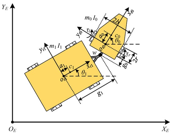
Figure 1.
Plane motion diagram of the tractor-trailer. (OEXEYE is the earth-fixed coordinate system. ot0xt0yt0 is the tractor-fixed coordinate system. ot1xt1yt1 is the trailer-fixed coordinate system. θ0 is the heading angle of the tractor. θ1 is the heading angle of the tractor. τl and τr are the driving torque of the left and right wheels of the tractor. r is the radius of driving wheels. 2b is the distance between two active wheels of the tractor. a0 is the distance of the centroid c0 and the midpoint ot0 of tractor wheel axle. a1 is the distance of the centroid c1 and the center point ot1 of the trailer. g0 is the distance between the hinge point w and the midpoint ot0 of tractor wheel axle. g1 is distance between the hinge point w and the center point ot1 of the trailer. m0 is the mass of the tractor. m1 is the mass of the trailer without load. I0 is the rotational inertia about vertical axis through c0. I1 is the rotational inertia about vertical axis through c1 when the trailer is not loaded).
In the system of the autonomous tractor-trailer, in addition to describing the position and direction variables of the tractor and trailer, the relative heading angle information of the tractor and trailer must also be considered. Based on the previous assumption (3)—the wheels of the tractor and trailer do not slip laterally—the following nonholonomic constraints can be obtained:
where x and y represent the position coordinates of the trailer, θ1 represents the heading angle of the trailer, and θ0 represents the heading angle of the tractor.
The posture vector of the tractor-trailer is defined as q = [x, y, θ1, θ0]T, and Equation (1) can be rewritten into the following matrix form:
where and it is the constraint matrix of the system.
In addition, we introduce a full rank matrix S(q) = [s1(q), s2(q)]T, which consists of a set of smooth and linearly independent vector fields, , i = 1, 2, in the null space of A(q), that is, A(q)S(q) = 0 [3]. We define the pseudo velocity vector υ(t) = [v(t), ω(t)]T as the input vector, and the system can be expressed as:
where v(t) represents the linear speed of ot point on the trailer, ω(t) represents the angular speed of the tractor, and S(q) is called the motion matrix.
2.2. Dynamic Model of Tractor-Trailer
The tractor-trailer system can be described by using the first Lagrange equation, which can be expressed as follows:
where fk represents the generalized force, λ represents the Lagrange multiplier, and k represents the number of generalized coordinates; L can be obtained by the following formula:
where represents the kinetic energy of the system and represents the potential energy of the system.
According to assumption (1) in Section 2.1, the tractor-trailer moves only on the horizontal plane, so its gravitational potential energy will not change. According to assumption (2) in Section 2.1, the tractor-trailer is composed of rigid parts, so its elastic potential energy can be regarded as zero. Therefore, the body kinetic energy of the tractor and trailer can be considered to establish the dynamic model. Based on Equations (4) and (5), the dynamic model of the tractor-trailer system can be given by:
where τd represents the unknown nonlinearity vector caused by external disturbances, ground friction, and so on; Ma1 represents the symmetric positive definite inertia matrix; Ca1 represents the matrix of centripetal force and Coriolis force; Da1 represents the matrix of damping and viscous friction coefficient; Ba1 represents the input transformation matrix; and τ = [τl, τr]T represents the input torque vector. To simplify the design, an on-axle hitching tractor-trailer (g0 = 0) is considered. Based on [3], the dynamic matrices are selected as follows:
where the model parameters can be defined as , , , , where the ml(t) represents the time-varying load on the trailer, Il(t) represents the rotational inertia on the trailer, and δa1(t) represents the unexpected change of the centroid of the trailer.
The derivative of Equation (3) with respect to time can be obtained , and then it can be substituted into Equation (6) and multiply ST(q) on both sides of the equation to eliminate the nonholonomic constraints in the model [21]. Finally, the simplified equation is as follows:
where , , , , .
2.3. Coordinate Transformation
In order to achieve the goal of trajectory tracking, it is necessary to construct a tracking error space based on the driving trajectory of the tractor-trailer and reference trajectory, and then derive the tracking error model. Let the state vector of the reference trajectory be qr = [xr, yr, θ1r, θ0r]T, the trajectory tracking error of the tractor-trailer can be expressed as qe = q − qr = [qe1, qe2, qe3, qe4]T = [xe, ye, θ1e, θ0e]T. We transform the posture errors between the driving trajectory of the tractor-trailer and the reference trajectory in the earth-fixed coordinate system (OEXEYE) are transformed into the trailer-fixed coordinate system (ot1xt1yt1) using the following transformation [3]:
The derivative of Equation (8) with respect to time is performed, and the Taylor series expansion is used at the reference trajectory point. The tracking error state space equation of the tractor-trailer after ignoring the higher-order term is as follows:
where , , .
2.4. Prescribed Performance Function
In order to improve the transient performance and final tracking error of the control system, the prescribed performance function is introduced to set the performance envelope of the controlled system, so that the tracking error will always be within the prescribed boundary range [20]. To achieve this, a strictly positive, bounded, smooth and decreasing performance function of time for each element of the tracking error vector , i.e., qej(t), j = 1, …, 4, to satisfy the following bounds:
where
and are some positive constants, indicating overshoot suppression parameters. The following smooth continuous and monotonically decreasing prescribed performance function ρj(t) is defined [22]:
Moreover, the prescribed performance function ρj(t) needs to meet the following conditions: (1) , ; (2) . Among them, ρj0, ρj∞ and lj are positive numbers. ρj0 represents the prescribed initial value, ρj∞ represents the prescribed maximum allowable steady-state error, and lj represents the convergence rate of tracking error.
The following form of error transformation is introduced to convert the inequality constraint shown in Equation (10) into the form of equality constraint:
where ζj represents the new conversion error; then, the error conversion function S(ζj) meets the following conditions [23]: (1) S(ζj) is a smooth and strictly monotone increasing function; (2) ; (3) , .
The selected error conversion function is as follows:
According to Equation (13), it can be further obtained:
where γj = qej(t)/ρj(t). Therefore, the new conversion error ζj can be obtained by error equivalence transformation, and the tracking error , i.e., qej(t), j = 1, …, 4 of the tractor-trailer is controlled within the predetermined boundary (Equation (10)) by designing the trajectory tracking controller. That is, the prescribed performance tracking control problem of the tractor-trailer system (Equation (9)) can be transformed into the stabilization problem of the equivalent error system (Equation (14)).
3. Main Results
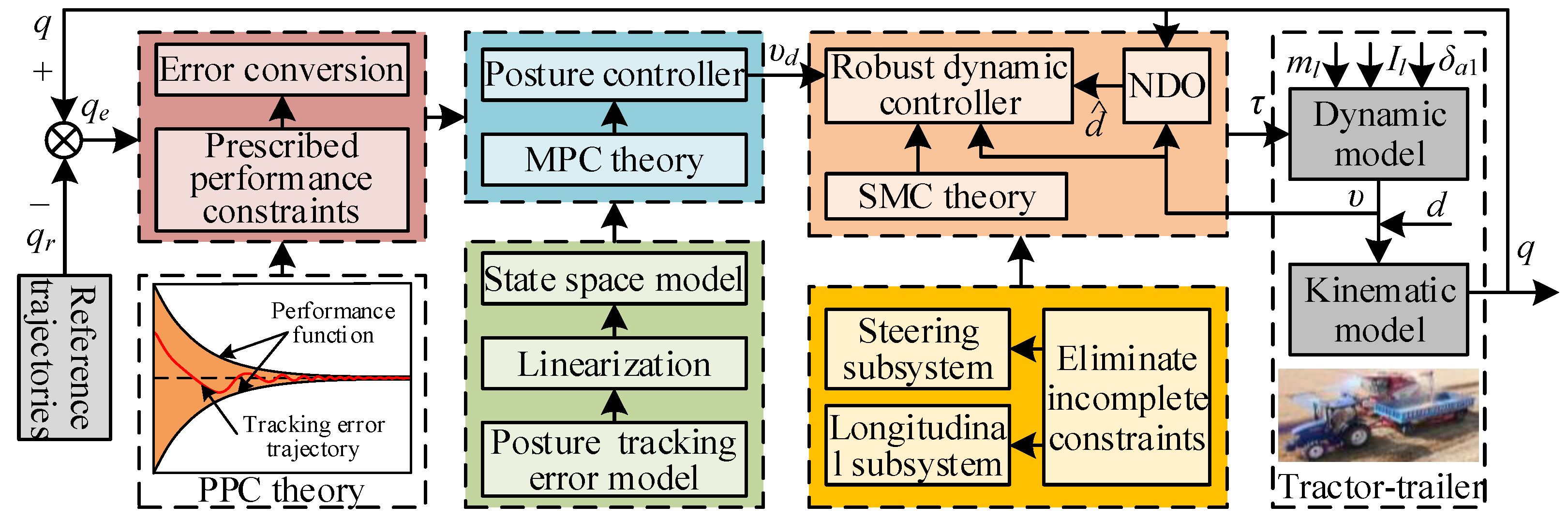
For a robot with simple structure, it is easy to obtain the analytical solution of the kinematic and dynamic models and achieve accurate and stable trajectory tracking control. However, it is difficult or even impossible to obtain the accurate kinematic and dynamic models in practical application because of the complex mechanical structure of the tractor-trailer and various uncertain disturbances. The past control methods have many disadvantages, such as complex control laws and high requirements for model accuracy. To solve these problems, a robust trajectory tracking control algorithm with double closed-loop structure is proposed, as shown in Figure 2. The PPC method uses a prescribed performance function to constrain deviations from the desired trajectory within a specified range. Combined with the posture tracking error model, the MPC method is selected to construct the posture controller. Then, the robust dynamic controller is designed based on SMC and NDO. Through the methods proposed in this paper, the posture tracking and driving torque control of the tractor-trailer can be realized simultaneously.
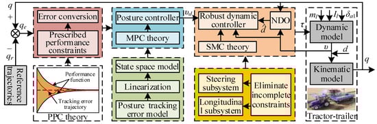
Figure 2.
Schematic diagram of the proposed robust tracking control system.
3.1. Posture Controller
The posture tracking error model of the tractor-trailer is shown in Equation (9); it is a continuous-time system. The forward difference method is used to discretize the above linear system, which can be expressed as follows:
where , , I represents the identity matrix and Ts represents the sampling step size of the discretization process.
To design the MPC controller, Equation (15) can be converted into the following new state space form:
where , , , , ΔU represents the increment of control input.
Define the prediction time domain as Np and the control time domain as Nc, then the output of the system at the future time can be expressed in the following matrix form [9]:
where , , , .
In order to avoid a situation where the optimal solution cannot be calculated, the following objective functions with soft constraints are designed:
where Q and R are the weight matrices, ρ is the weight coefficient, and ε is the relaxation factor.
To obtain a standard quadratic programming model with inequality constraints, we transform the objective function using Equation (19). At the same time, considering the dynamic constraints and actuator constraints in the trajectory tracking control process of the tractor-trailer, the system control quantities and control increment constraints are set.
where , it is a Hessian matrix, and describes the quadratic term of the objective function; , it describes the linear part of the objective function.
By solving Equation (19), a series of control input increments in the control horizon can be obtained as . Subsequently, we set the first element of the control sequence as the actual control input increment of vehicle system, given by [5]:
Then, the corresponding control input of the posture controller can be ultimately obtained by:
3.2. Dynamic Controller
The goal of the inner loop dynamic controller is to track the desired speed signal υd generated by the outer loop posture controller by controlling the driving torque on both sides of the tractor-trailer. The uncertainty of model parameters and internal and external disturbances will also affect the performance of the dynamic controller. In this section, the NDO is designed to estimate the total disturbance in the system to achieve disturbance compensation. At the same time, considering the advantages of SMC, such as strong robustness, simple design process, and low model dependency, the dynamic controller will be designed based on the SMC method.
3.2.1. Design of NDO
The dynamic model Equation (7) of the tractor-trailer can be rewritten as follows:
where is the unknown disturbance term.
The basic design idea of the disturbance observer is to correct the estimated value by the difference between the actual output and the estimated output. Assuming that the time-varying unknown disturbance d is bounded and continuously differentiable, the observation error of the disturbance observer is defined as
, and the linear disturbance observer is designed as [24]:
Generally, there is no differential prior knowledge of disturbance. Relative to the dynamic characteristics of the disturbance observer, we can assume that the change of disturbance is slow, that is, . Then, the dynamic equation of observation error is as follows:
where L(υ) represents observation error gain.
Further, the following NDO can be designed:
where is the estimated value of the unknown disturbance d; z is the intermediate variable of the NDO; g(υ) is the nonlinear function to be designed; L(υ) is the gain coefficient of the NDO; and L(υ) = ∂g(υ)/∂t. L(υ) is selected as a constant, the design function g(υ) = L(υ − υ0), and υ0 is the initial value of the state variable.
According to Equations (23) and (24), the dynamic equation of observation error of NDO can be obtained as follows:
Through the above Equation (26), we can get , where c is a constant. Therefore, if L(υ) > 0, the observation error of the NDO can be converged, and the convergence rate can be determined by selecting the design parameter L(υ) [25].
3.2.2. Design of Sliding Mode Controller
According to the dynamic model shown in Equation (7), the tractor-trailer can be divided into two subsystems: longitudinal speed and steering angular speed, and the corresponding tracking error can be defined as follows:
Select the sliding mode surface in the form of proportional-integral as follows [9]:
where is positive weight coefficient.
The derivative of the Equation (28) regarding time is shown as follows:
To reduce the chattering of the sliding mode surface, we choose a fast power reaching law with second-order sliding mode characteristics to ensure better dynamic characteristics in the reaching stage [26,27]; it is shown as follows:
where κ11, κ12, κ21 and κ22 are constants greater than zero, α1∈(0, 1), α2∈(0, 1).
According to Equations (7), (29), and (30), the driving torque control law of the tractor-trailer can be expressed as follows:
where is the unknown disturbance term.
As mentioned earlier, in Equation (31) is abbreviated as d, and the NDO is designed to estimate it. Therefore, the final driving torque control law of the tractor-trailer can be expressed as follows:
In order to analyze the stability of the designed SMC, we select the Lyapunov function presented as:
The derivative of Equation (33) regarding time is shown as follows:
Therefore, according to the Lyapunov stability principle and LaSalle invariance theorem, it can be concluded that all signals are bounded and the velocity error can converge to zero with time.
4. Results and Analysis
4.1. Simulation Description
Assume that the trajectory of the trailer in the tractor-trailer meets the following equation:
According to the geometric relationship, the tractor in the tractor-trailer should meet the following constraints [21]:
According to Ref. [3], the model parameters of the tractor-trailer used in the simulation are defined as follows: r = 0.45 m, b = 0.8 m, a0 = 0.45 m, a1 = 0.25 m, g0 = 0 m, g1 = 3 m, m0 = 700 kg, m1 = 450 kg, I0 = 280 kg·m2, I1 = 180 kg·m2. The actuator input signals of the posture controller are saturated |v| ≤ 5 m/s and |ω| ≤ 4 rad/s, respectively. The actuator input signals of the dynamic controller are also saturated |τl| ≤ 200 N·m and |τr| ≤ 200 N·m, respectively. The reference trajectory for the tractor-trailer begins at the initial posture q = [0.5, 11, 0, 0]T.
Considering the existence of uneven ground, load interference, sensor measurement error, and other disturbances in the actual farmland environment, the following interference and noise vectors are selected to be added to the model of the tractor-trailer:
As autonomous navigation technology has developed, there are more and more scenarios where the tractor-trailers need to work together with other vehicles, such as combine harvesters and tractor-trailers working together to unload grain. At this time, in addition to the influence of internal and external disturbances, the model parameters such as the mass, rotational inertia, and centroid of the tractor-trailer will change greatly. The following Equation (38) is used to simulate the change of trailer mass and rotational inertia in the trajectory tracking control process of the tractor-trailer:
where Ts = 20 s and Tf = 80 s are the start and stop times of the crop loading. H(t) is the Heaviside step function [3].
The sample time T = 0.05 s. The prescribed performance functions are used with parameter values of ρ10 = 0.5, ρ1∞ = 0.1, l1 = 1, , , ρ20 = 1, ρ2∞ = 0.1, l2 = 1, , , ρ30 = 0.5, ρ3∞ = 0.1, l3 = 1.5, , , ρ40 = 0.5, ρ4∞ = 0.1, l4 = 1.5, , . The parameters of posture controller based on the MPC method are selected as the predictive horizon Np = 15, the control horizon Nc = 5, the weight matrix Q = 100 × I60, R = I30 and ρ = 10. Moreover, the parameters of the dynamic controller based on the SMC method and NDO are selected as β1 = 5, β2 = 5, κ11 = 3, κ12 = 0.1, κ21 = 3, κ22 = 0.1, α1 = 0.2, α2 = 0.2, L = 100 × I2.
4.2. Simulation Results
4.2.1. NDO
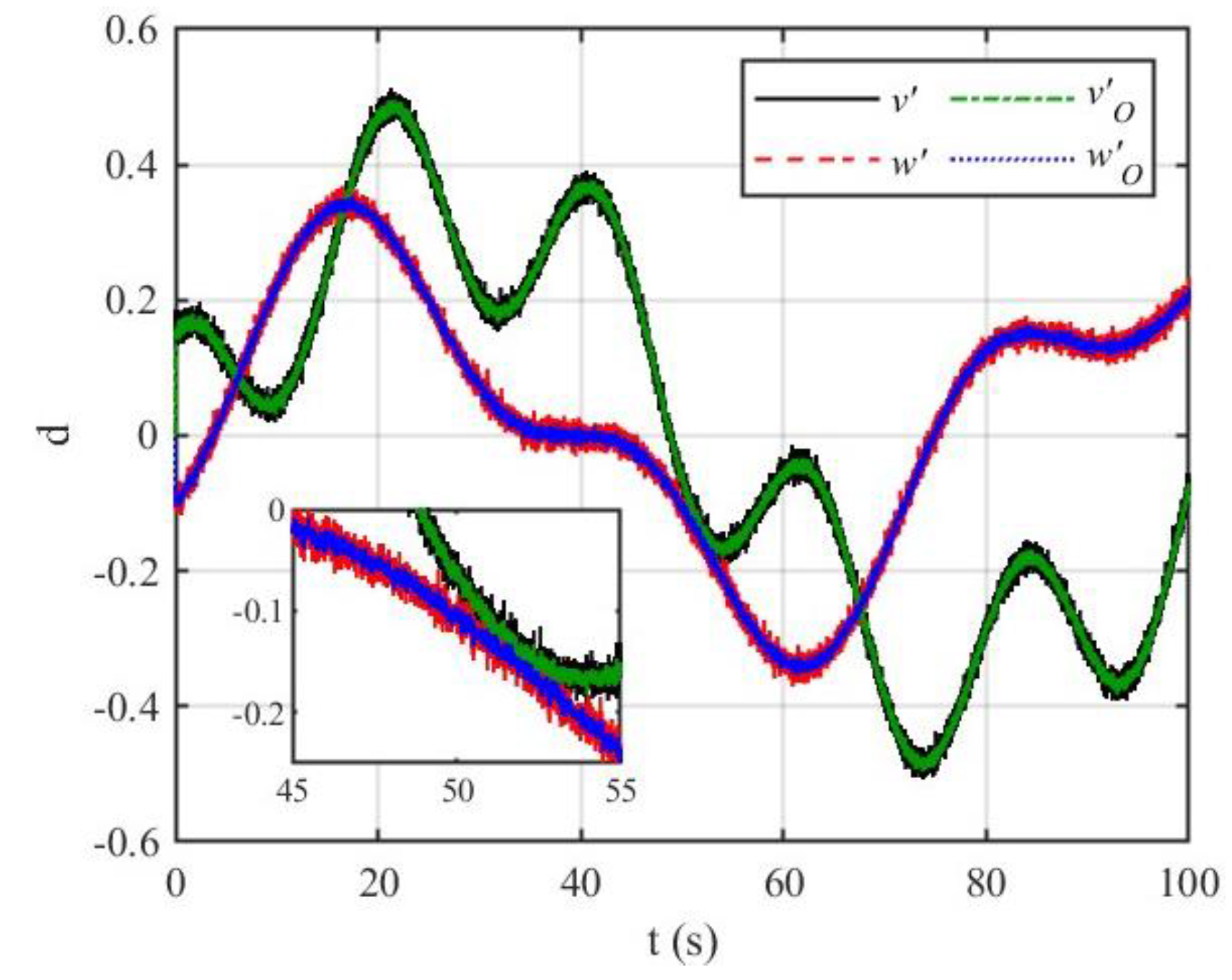
Before the trajectory tracking control simulation of the tractor-trailer, we need to prove the effectiveness of the NDO designed in this paper. First of all, suppose that there is no change in the model parameters of the tractor-trailer during driving; the system disturbance is shown in Equation (37), and the disturbance observation results are shown in Figure 3. In Figure 3, the black solid line and red dashed line are the system disturbance curves added in the simulation, and the green dash-dotted line and blue dotted line are the observed value curves of the system disturbance. It shows that the proposed NDO can successfully realize the disturbance observation of the tractor-trailer system.

Figure 3.
Disturbance observation curves of the tractor-trailer without considering the model parameter changes.
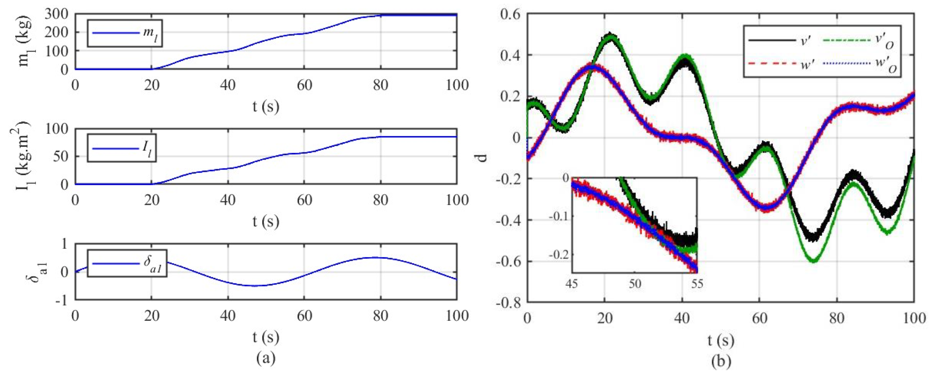
In some special application scenarios, for example, during the cooperative operation of the tractor-trailer and the combine harvester, the combine harvester will synchronously transport the grain to the trailer of the tractor-trailer. At this time, the mass, rotational inertia, and centroid of the trailer change significantly, and the simulated incremental change process is shown in Figure 4a, and the disturbance observation results are shown in Figure 4b. It can be seen from Figure 4b that the observation curve of the NDO in the angular velocity direction is consistent with the added disturbance curve, but the observation curve of the NDO in the velocity direction is inconsistent with the added disturbance. This is because the model parameter changes affect the size of the actual disturbances in the tractor-trailer. Therefore, the changes in model parameters can be incorporated into system disturbances, so that the actual disturbances of the tractor-trailer can be observed using the NDO designed in this paper. At the same time, it also reflects that the idea of designing the NDO to estimate the system disturbances and compensate them to the control system is correct.
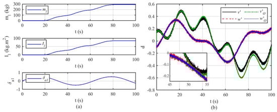
Figure 4.
Disturbance observation curves of the tractor-trailer considering the model parameter changes: (a) the change curves of model parameters; (b) the observation curves of system disturbances.
4.2.2. Robust Tracking Control
In order to verify the effectiveness of the method proposed in this paper, it is compared with the control method in Refs. [5,9]. In the following simulation results, the legend Ref. represents the reference input, the legend MS represents the method proposed in Ref. [9], the legend RTMS represents the method proposed in Ref. [5], and the legend PMSO represents the method proposed in this paper.
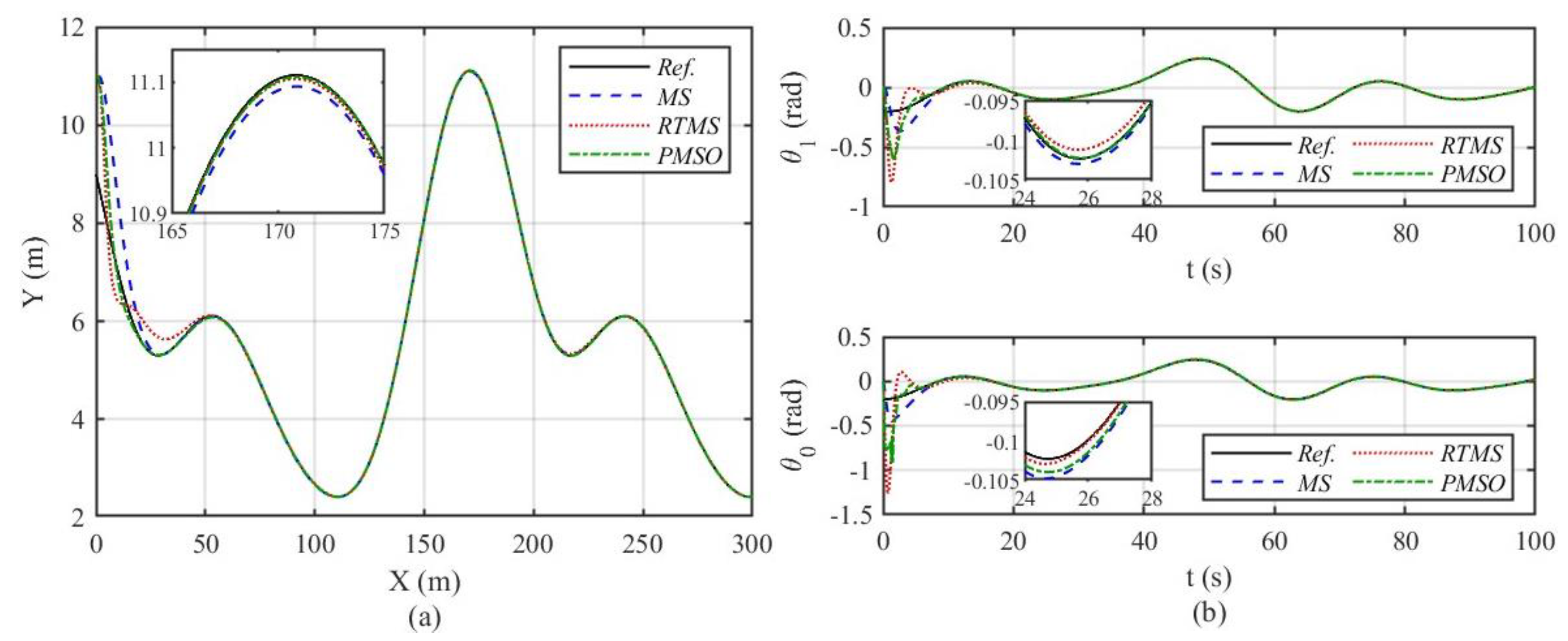
According to the reference trajectories shown in Equations (35) and (36), the trajectory tracking control results of the tractor-trailer are shown in Figure 5. It can be seen from the position control curves in Figure 5a that the three control methods (MS-Ref. [9], RTMS-Ref. [5], PMSO-this paper) can successfully achieve high-precision trajectory tracking control, but the method proposed in this paper has the fastest response speed. In Figure 5b, the heading tracking control errors of the control method in Ref. [9] is the smallest at the beginning, but the response speed is the slowest. The Ref. [5] and the method proposed in this paper have faster response speed, but have larger tracking error at the beginning, and the tracking error of the method proposed in this paper is smaller.
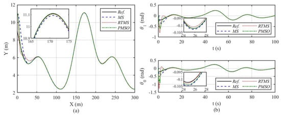
Figure 5.
Trajectory tracking control results of the tractor-trailer: (a) position control curves; (b) heading control curves.
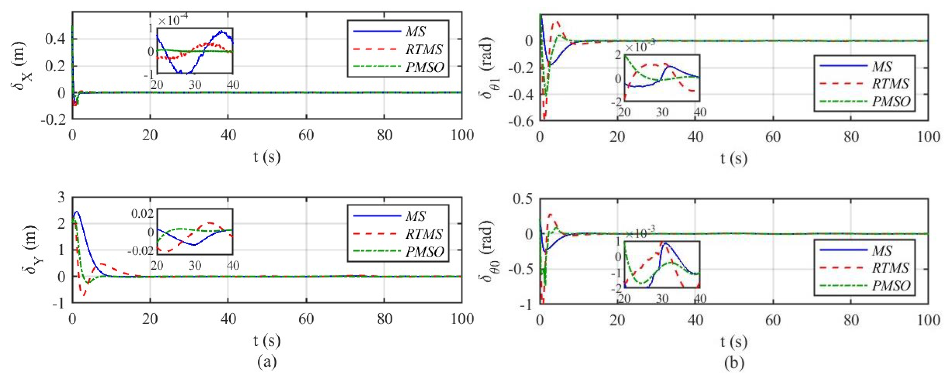
The tracking control errors of the tractor-trailer are shown in Figure 6. It can be seen from the position error curves in Figure 6a that the method proposed in this paper has a faster response speed and better tracking error stability than the methods in Refs. [5,9]. At the same time, they also prove the goal of the transient and steady-state performance constraint specified by the prescribed performance function. Similarly, the heading error curves in Figure 6b also prove this point.
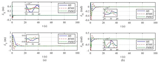
Figure 6.
Tracking control errors of the tractor-trailer: (a) position error curves; (b) heading error curves.
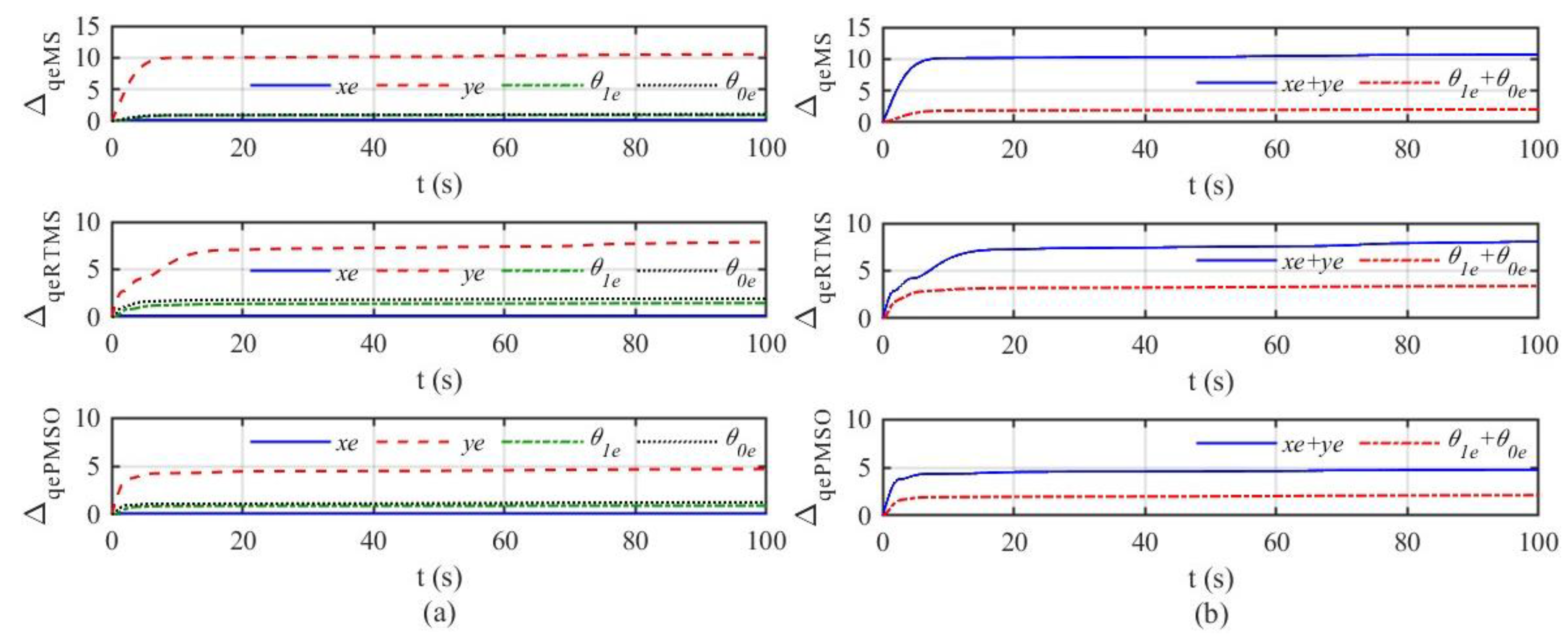
In order to better illustrate the effectiveness of the method proposed in this paper, we have calculated the cumulative tracking control errors of the tractor-trailer, as shown in Figure 7. It can be seen from the cumulative posture error curves in Figure 7a that the cumulative posture errors rise rapidly at the beginning of control, and then reaches the stable tracking control stage. Furthermore, the subsequent cumulative posture errors basically do not increase, reflecting that the three control methods (MS-Ref. [9], RTMS-Ref. [5], PMSO-this paper) can achieve the stable and high-precision trajectory tracking control of the tractor-trailer. However, the cumulative posture errors of the proposed method in this paper are the smallest, which shows it has higher robustness and better performance. Then, we sum the position errors (xe, ye) and heading errors (θ1e, θ0e), respectively, to obtain Figure 7b. Similarly, the cumulative error curves of position and heading in Figure 7b also prove the effectiveness of the method proposed in this paper.
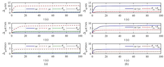
Figure 7.
Cumulative tracking control errors of the tractor-trailer: (a) cumulative posture error curves; (b) cumulative error curves of position and heading.
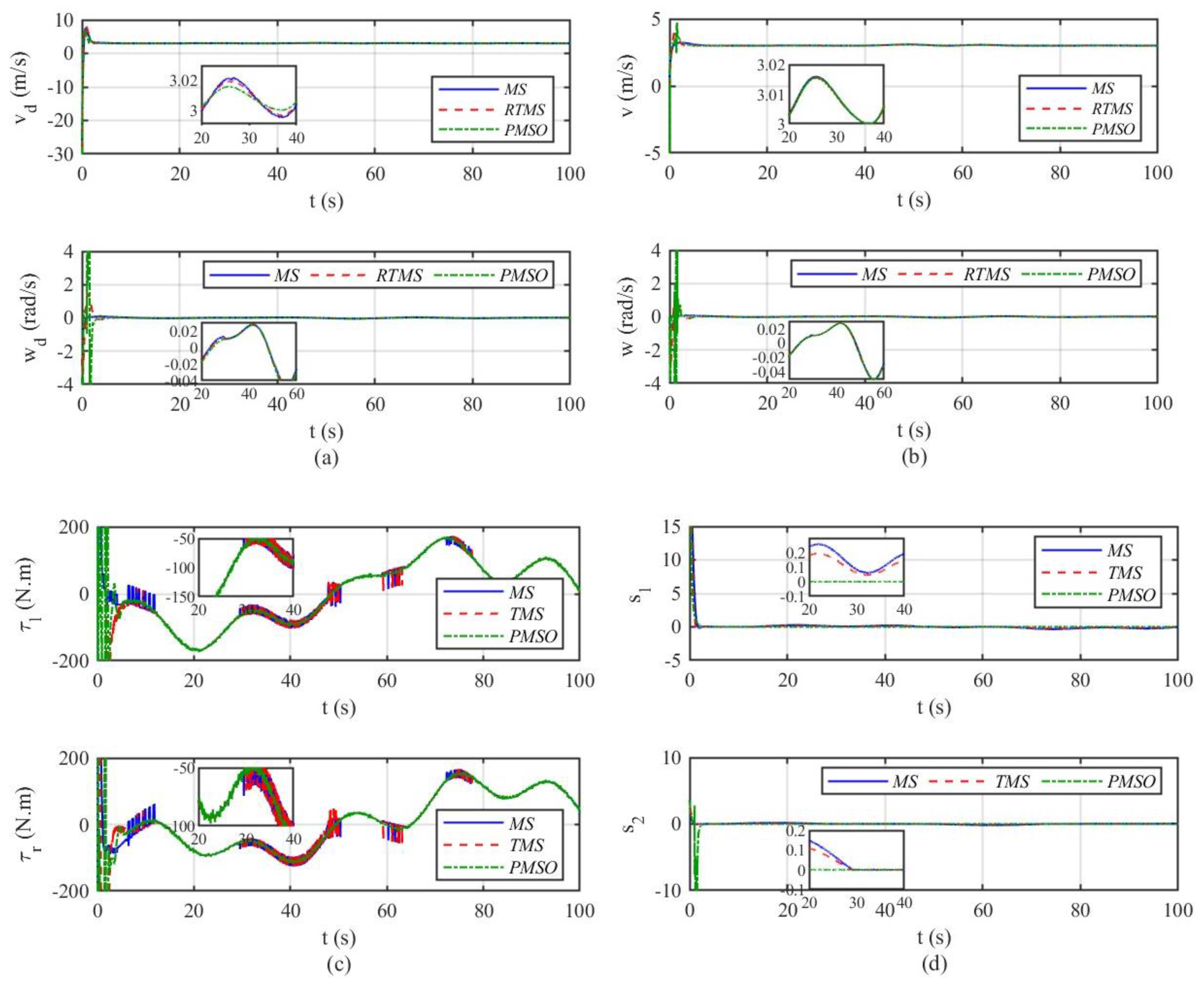
The control quantities of the posture controller and dynamic controller of the tractor-trailer are shown in Figure 8. Figure 8a shows the control outputs of the posture controller. It can be seen from Figure 8a that the method proposed in this paper has changed greatly in the initial stage compared with the methods in Refs. [5,9], because the tractor-trailer has large initial trajectory tracking errors. In order to meet the prescribed transient and steady-state performances, the prescribed performance function used in this paper will restrict the tracking error, which leads to this phenomenon. However, when the trajectory tracking control reaches the stable stage, the method proposed in this paper shows better robustness and steady-state performance. Figure 8b shows the actual speed and angular speed of the tractor-trailer based on the three control methods (MS-Ref. [9], RTMS-Ref. [5], PMSO-this paper). Figure 8c shows the control outputs of the dynamic controller. It can be seen that compared with the traditional sliding mode reaching law in Ref. [9], the control output curves of the proposed fast power reaching law with second-order sliding mode characteristics are smoother and achieve the purpose of reducing chattering. Figure 8d shows the sliding mode surfaces of the dynamic controller.
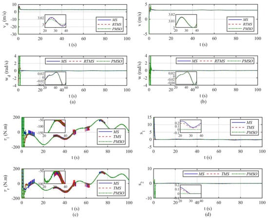
Figure 8.
Control quantities of the posture controller and dynamic controller of the tractor-trailer: (a) control outputs of the posture controller; (b) actual speed and angular speed of the tractor-trailer; (c) control outputs of the dynamic controller; (d) sliding mode surfaces of the dynamic controller.
5. Conclusions
Aiming at the requirement of stable and high-precision tracking control of tractor-trailer vehicles in modern agriculture, this paper studies the robust trajectory tracking control of autonomous tractor-trailer systems. Based on the derived kinematic and dynamic model, the double closed-loop control structure is designed, the MPC method is used to construct the posture controller, and the SMC method and NDO strategy are used to construct the dynamic controller. Moreover, the convergence speed and final tracking control accuracy of the tractor-trailer control system can be guaranteed by an effective application of the PPC technique.
The disturbance observation results show the designed NDO can precisely estimate the system disturbances. The comparative simulation results show that under the proposed control method in this paper, even with system disturbances, the tractor-trailer can track the reference trajectory well. The tracking control error curves show that the method proposed in this paper has faster response speed and better tracking error stability than the other two control methods. At the same time, they also prove the goal of the transient and steady-state performance constraint achieved by the prescribed performance function. The cumulative tracking control error curves show that the cumulative errors of the proposed method are the smallest, and show higher robustness and better performance. In addition, the control output curves of the dynamic controller show that the proposed fast power reaching law with second-order sliding mode characteristics are smoother and achieve the purpose of reducing chattering. In future work, we plan to carry out application research under complex working conditions, and focus on controller saturation, time delay, control parameter optimization, and other related issues.
Author Contributions
Conceptualization, E.L. and J.X.; methodology, E.L.; software, T.C.; investigation, S.J.; writing—original draft preparation, J.X.; writing—review and editing, E.L. All authors have read and agreed to the published version of the manuscript.
Funding
This research was funded by the National Natural Science Foundation of China (Grant No. 52005220), the National Key Research and Development Program of China (Grant No. 2022YFD00150402), and A Project Funded by the Priority Academic Program Development of Jiangsu Higher Education Institutions (Grant No. PAPD-2018-87).
Data Availability Statement
Data available on request from the authors.
Conflicts of Interest
The authors declare no conflict of interest.
References
- Bechar, A.; Vigneault, C. Agricultural robots for field operations: Concepts and components. Biosyst. Eng. 2016, 149, 94–111. [Google Scholar] [CrossRef]
- Lu, E.; Ma, Z.; Li, Y.M.; Xu, L.Z.; Tang, Z. Adaptive backstepping control of tracked robot running trajectory based on real-time slip parameter estimation. Int. J. Agric. Biol. Eng. 2020, 13, 178–187. [Google Scholar] [CrossRef]
- Shojaei, K. Intelligent coordinated control of an autonomous tractor-trailer and a combine harvester. Eur. J. Control. 2021, 59, 82–98. [Google Scholar] [CrossRef]
- Yuan, J.; Sun, F.C.; Huang, Y.L. Trajectory generation and tracking control for double-steering tractor-trailer mobile robots with on-axle hitching. IEEE Trans. Ind. Electron. 2015, 62, 7665–7677. [Google Scholar] [CrossRef]
- Yue, M.; Hou, X.Q.; Zhao, X.D.; Wu, X.M. Robust tube-based model predictive control for lane change maneuver of tractor-trailer vehicles based on a polynomial trajectory. IEEE Trans. Syst. Man Cybern. Syst. 2018, 50, 5180–5188. [Google Scholar] [CrossRef]
- Alipour, K.; Robat, A.B.; Tarvirdizadeh, B. Dynamics modeling and sliding mode control of tractor-trailer wheeled mobile robots subject to wheels slip. Mech. Mach. Theory 2019, 138, 16–37. [Google Scholar] [CrossRef]
- Kassaeiyan, P.; Alipour, K.; Tarvirdizadeh, B. A full-state trajectory tracking controller for tractor-trailer wheeled mobile robots. Mech. Mach. Theory 2020, 150, 103872. [Google Scholar] [CrossRef]
- Murillo, M.; Sánchez, G.; Deniz, N.; Genzelis, L.; Giovanini, L. Improving path-tracking performance of an articulated tractor-trailer system using a non-linear kinematic model. Comput. Electron. Agric. 2022, 196, 106826. [Google Scholar] [CrossRef]
- Liu, Z.Y.; Yue, M.; Guo, L.; Zhang, Y.S. Trajectory planning and robust tracking control for a class of active articulated tractor-trailer vehicle with on-axle structure. Eur. J. Control. 2020, 54, 87–98. [Google Scholar] [CrossRef]
- Zhang, R.X.; Xiong, L.; Yu, Z.P.; Bai, M.F.; Fu, Z.Q. Robust trajectory tracking control of autonomous vehicles based on conditional integration method. J. Mech. Eng. 2018, 54, 129–139. [Google Scholar] [CrossRef]
- Liao, J.F.; Chen, Z.; Yao, B. Model-based coordinated control of four-wheel independently driven skid steer mobile robot with wheel-ground interaction and wheel dynamics. IEEE Trans. Ind. Inform. 2019, 15, 1742–1752. [Google Scholar] [CrossRef]
- Elhaki, O.; Shojaei, K. Output-feedback robust saturated actor-critic multi-layer neural network controller for multi-body electrically driven tractors with n-trailer guaranteeing prescribed output constraints. Robot. Auton. Syst. 2022, 154, 104106. [Google Scholar] [CrossRef]
- Taghia, J.; Wang, X.; Lam, S.; Katupitiya, J. A sliding mode controller with a nonlinear disturbance observer for a farm vehicle operating in the presence of wheel slip. Auton. Robot. 2017, 41, 71–88. [Google Scholar] [CrossRef]
- Korayem, A.H.; Khajepour, A.; Fidan, B. Trailer mass estimation using system model-based and machine learning approaches. IEEE Trans. Veh. Technol. 2020, 69, 12536–12546. [Google Scholar] [CrossRef]
- Han, S.; Yoon, K.; Park, G.; Huh, K. Hybrid state observer design for estimating the hitch angles of tractor-multi unit trailer. IEEE Trans. Intell. Veh. 2022, 8, 1449–1458. [Google Scholar] [CrossRef]
- Guevara, L.; Jorquera, F.; Walas, K.; Auat-Cheein, F. Robust control strategy for generalized N-trailer vehicles based on a dual-stage disturbance observer. Control Eng. Pract. 2023, 131, 105382. [Google Scholar] [CrossRef]
- Guo, Y.K.; He, S.D.; Dai, S.L. Finite-time synchronization of nonlinear multi-agent systems with prescribed performance. In Proceedings of the 38th Chinese Control Conference, Guangzhou, China, 27–30 July 2019; pp. 5635–5640. [Google Scholar]
- Bechlioulis, C.P.; Rovithakis, G.A. Robust adaptive control of feedback linearizable MIMO nonlinear systems with prescribed performance. IEEE Trans. Autom. Control 2008, 53, 2090–2099. [Google Scholar] [CrossRef]
- Shojaei, K.; Abdolmaleki, M. Output feedback control of a tractor with N-trailer with a guaranteed performance. Mech. Syst. Signal Process. 2020, 142, 106746. [Google Scholar] [CrossRef]
- Guo, G.; Zhang, Q.; Gao, Z.Y. Finite-time fixed configuration formation control of intelligent vehicles with prescribed transient and steady-state performance. China J. Highw. Transp. 2022, 35, 28–42. [Google Scholar]
- Yue, M.; Wu, X.M.; Guo, L.; Gao, J.J. Quintic polynomial-based obstacle avoidance trajectory planning and tracking control framework for tractor-trailer system. Int. J. Control. Autom. Syst. 2019, 17, 2634–2646. [Google Scholar] [CrossRef]
- Yin, Z.Y.; Suleman, A.; Luo, J.J.; Wei, C.S. Appointed-time prescribed performance attitude tracking control via double performance functions. Aerosp. Sci. Technol. 2019, 93, 105337. [Google Scholar] [CrossRef]
- Chen, L.S.; Ning, X.M. Nonlinear PI cascade attitude control with prescribed performance for a quadrotor UAV. J. Appl. Sci. 2019, 37, 137–150. [Google Scholar]
- Jin, Z.J.; Liu, S.; Zhang, L.H.; Lan, B.; Qin, H.R. Command-filtered backstepping control for stabilization of ship rolling based on nonlinear disturbance observer. Shipbuild. China 2019, 60, 121–130. [Google Scholar]
- Li, C.X.; Meng, X.Y.; Wang, J. Design of aircraft trajectory tracking controller based on disturbance observer. Syst. Eng. Electron. 2022, 44, 2593–2600. [Google Scholar]
- Li, P. Research and Application of Traditional and Higher-Order Sliding Mode Control; National University of Defense Technology: Changsha, China, 2011. [Google Scholar]
- Lu, E.; Li, W.; Yang, X.F.; Liu, Y.F. Anti-disturbance speed control of low-speed high-torque PMSM based on second-order non-singular terminal sliding mode load observer. ISA Trans. 2019, 88, 142–152. [Google Scholar] [CrossRef] [PubMed]

Disclaimer/Publisher’s Note: The statements, opinions and data contained in all publications are solely those of the individual author(s) and contributor(s) and not of MDPI and/or the editor(s). MDPI and/or the editor(s) disclaim responsibility for any injury to people or property resulting from any ideas, methods, instructions or products referred to in the content. |
© 2023 by the authors. Licensee MDPI, Basel, Switzerland. This article is an open access article distributed under the terms and conditions of the Creative Commons Attribution (CC BY) license (https://creativecommons.org/licenses/by/4.0/).