Design and Experimental Study of Ball-Head Cone-Tail Injection Mixer Based on Computational Fluid Dynamics

Abstract

The uniform and accurate mixing of pesticides in water is a necessary prerequisite for plant protection, especially for enabling precise variable spraying, and is also an important method to achieve a precise reduction in pesticide spraying. In order to ensure the uniform mixing of pesticides and water and solve the problems of traditional injection mixers, such as the limited range in the mixing ratio and unadjustable proportion, an active injection liquid mixer is designed in this paper. The mixer can be matched with an online mixing and spraying device to achieve accuracy in mixing and spraying. In this paper, a computational fluid dynamics (CFD) method is used to optimize the structure of the mixer. Through comparative analysis, the optimal structure of the mixer was found. It has a spherical head and conical tail, the number of guide plates is seven, and the shape is semicircular. By calculating the volume fraction of pesticide distribution under different cross-sections, the coefficient of variation in the process of mixing is obtained. The analysis shows that the maximum coefficient of variation of the ball-head cone-tail active injection mixer was 2.88% (lower than the allowable 5%) with a mixing ratio ranging from 300:1 to 3000:1. At the same time, image analysis methods of high-definition photography and ultraviolet spectrophotometry were used to analyze the mixing effect of the mixer. The test results show that, when the pressure of the pesticide injection is 1 MPa, the distribution of the pesticide and water in the ball-head cone-tail injection mixer is more uniform under different mixing ratios, and it has a better spatio-temporal distribution uniformity with the concentration changing a little at different times and different spatial locations. The mixer can provide a theoretical reference and technical support for the subsequent realization of an accurate online variable spray.

1. Introduction

The uniform mixing of pesticides and water plays a key role in the spraying of agricultural plant protection, through which the damage of pests, diseases and weeds to crops can be effectively controlled [1,2,3]. There are many ways to mix pesticides and water. A traditional one is the premixed method, in which the operator puts pesticides and water together in a large medicine cabinet with a certain proportion. The operator may be exposed to the danger of pesticide pollution and burdened with a relatively high labor intensity, and the mixing effect cannot be guaranteed [4]. Then, the online mixing technology emerged. It is applied to separate the medicine box from the water tank, avoid direct contact between the operator and the pesticide, and improve the mixing effect at the same time [5,6]. More and more researchers have begun to study the mixing uniformity and precise ratio of pesticides and water to improve the utilization rate of pesticides and reduce the losses and pollution from pesticides.

The mixer is one of the main parts of the pesticide online mixing system, which is mainly used to guarantee the uniform mixing and accurate ratio of pesticides and water [7]. At present, the mixing methods of mixers mainly include injection mixing and jet mixing. The jet mixer has a simple structure and relatively high reliability, but, due to its structural limitations, it still has certain shortcomings in controlling the mixing ratio and dosage [8,9]. The injection mixer mainly uses external hardware to directly inject pesticides into water, so as to achieve the required mixing effect [10]. Compared with the jet mixer, it is superior in its intelligence and controllability with intelligent technology used to control the opening and closing of the injection valve to adjust the concentration of mixed pesticides [11]. Many researchers use computational fluid dynamics (CFD) simulation, optimization algorithms and numerical optimization to optimize the structure of jet mixers, which can reduce the pressure drop and shear strength and improve mixing efficiency [12,13,14,15,16]. There are also many experts and scholars optimizing the design of factors such as the geometry, nozzle angle and position of jet mixers, so as to improve the mixing efficiency and reduce the pressure drop [17,18,19]. However, the mixers still have some problems, such as unstable mixing, a large energy loss, and the low and unadjustable ratio of pesticide and water. The structural optimization of injection mixers has also been extensively studied internationally, in which the mixing effect and energy loss of mixers can be improved by changing the geometry of the inner cavity of the mixer and the position, shape and number of guide plates [20,21,22,23,24]. Han et al. [25] adopted numerical simulation and pilot scale test methods to optimize the structure of the static mixing device, to improve the mixing effect and save energy. Dai Xiang et al. [26] used the CFD method to simulate the movement and mixing of the fluid inside the injection mixer, which quantitatively described the mixing uniformity and further optimized the structure of the mixer. However, the injection mixer still has some problems such as high costs, a complex structure and an insufficient mixing uniformity. Therefore, in order to solve these problems, an injection liquid mixer with a simple structure, good mixing effect, high stability, large mixing ratio range and adjustable mixing ratio is designed in this paper.

In this paper, CFD software is used to simulate the mixing effect of mixers with different structural parameters. The effects of different head structures and different shapes, numbers, heights and angles of guide plates on the mixing uniformity, pressure drop and coefficient of variation are studied via single-factor analysis. Then, the coefficient of variation of mixing uniformity is analyzed in the mixing ratio range of 300:1~3000:1 with the optimal value as the parameter. Finally, the mixing effect of the mixer is analyzed qualitatively and quantitatively using the image analysis methods of high-definition photography and ultraviolet spectrophotometry.

The injection mixer designed in this study can achieve a precise reduction in pesticides and provide a theoretical reference and technical support for the subsequent realization of accurate online variable spraying.

2. Structural Design and Numerical Simulation of the Mixer

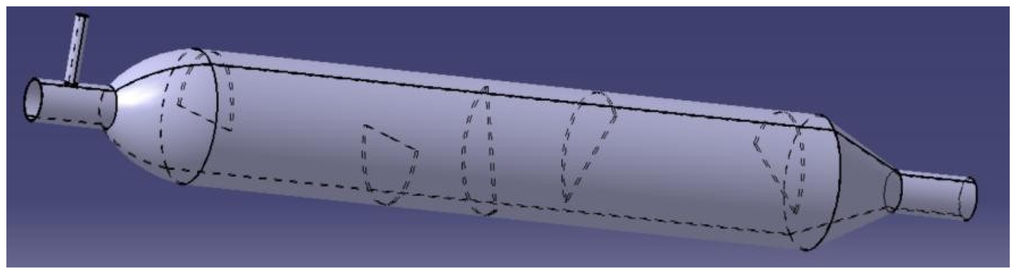
2.1. Structural Design of the Mixer

Referring to the relevant literature [27,28,29,30], this paper proposes to optimize the design of the built-in spoiler plate mixer. The overall cylindrical shape is chosen to ensure the formation of an internal pipeline flow field while allowing for easy processing and assembly with its external structure. Further optimization is performed on the head part of the mixer and the internal flow guide plates to improve the mixing effect. Considering the use of a ball head or cone head for interface transition, the use of a ball head or cone head at the entrance can better ensure that, when pesticides and water enter into the mixer, they will help the original flow rate in the mixer to form a cutting impact turbulent flow field as soon as possible and form a flow field diffusion effect similar to jet mixing. The exit part is also planned to have a spherical or conical finish, which assists in establishing a complete and continuous mixture flow at the end of the mixer. Meanwhile, a shrinking tube effect similar to jet mixing is established at the exit position to increase the flow velocity at the exit and further ensure the uniformity of mixing. Additionally, semicircular or isosceles-shaped orifice plates are proposed to create an irregular turbulent flow field in the internal flow field to accelerate mixing.

The injection mixer designed in this paper belongs to the category of the static mixer in principle. Based on the design principles and standards of the static mixer [31], the ratio of length to diameter of the mixer should be 7–10. And considering the actual size of the mixer installed on the matched mixing system, the size of the mixer should match the diameter of the water pipes at the two ends and that of the pipes delivering pesticides, as shown in

Table 1. Structure dimension parameters of the mixer.

Mixer Structure	Dimension Parameter (mm)
Cylindrical body length	500
Cylindrical body bore diameter	100
Head structure length	65
Water injection length	60
Water injection pipe diameter	32
Injection port length	50
Injection port diameter	10
Mixing outlet length	60
Mixed outlet pipe diameter	32

.

The center of the pesticide injection port is located on the axis of the mixer and perpendicular to the mixer to ensure that the liquid is injected directly into the water through the pesticide injection port. In addition, the internal structure of the cylindrical body is provided with a certain number of semicircular or isosceles-shaped guide plates. The semicircular guide plates’ diameters are consistent with the inner diameter of the main inner cavity of the mixer, and the isosceles-shaped guide plate is an isosceles trapezoidal plate whose bottom is fitted to the surface of the main inner cavity of the mixer. It is known that the mixing effect of staggered baffle blades is better than that of a sequential arrangement [32]. In this paper, the baffle is arranged along the axial direction of the mixer according to the helix with equidistance, and the thickness of all the baffles is designed to be 4 mm. On this basis, four kinds of mixers with the ball-head cone-tail shape, cone-head cone-tail shape, ball-head ball-tail shape and cone-head ball-tail shape are designed and compared. Figure 1 shows the structural model of the ball-head cone-tail injection mixer and the layout diagram of the internal baffle.

2.2. Numerical Simulation of the Mixer

2.2.1. CFD Mathematical Modeling

Considering the different head structures of the mixer and the different heights, angles, shapes and quantities of the baffle, SolidWorks software was used to model the different mixer structures in a 1:1 three-dimensional entity. Based on the total number of sprinkler heads of the spraying system attached to the mixer, the theoretical maximum flow rate of the spraying system in a fully open mode was calculated to be 144 L·min⁻¹, the required mixing ratio ranged from 300:1 to 3000:1, and the diameter of the main water pipe of the online mixing system that matches was 32 mm, while the output diameter of the medicine pump was 10 mm. By applying the Reynolds coefficient (Formula (1)) and the turbulence intensity (Formula (2)), the corresponding Reynolds number was 29,541, indicating a typical turbulent flow field. Therefore, the k-ε turbulent mixing model was selected for the simulation.

$$Re=\frac{D\rho }{\mu }\times \frac{v_1+v_2}{\frac{1}{4}\pi D^2\times 3600},$$

(1)

$$\mathrm{I}={0.16 \left(\mathrm{Re}\right) }^{-\frac{1}{8}},$$

(2)

where $Re$ is the Reynolds coefficient; $v_1 \mathrm{and} v_2$ are the volume flow rates of pesticide and water (m³·h⁻¹), respectively; $D$ is the mixer diameter; $\mu$ is the coefficient of liquid viscosity; $\rho$ is the density of the liquid; and $\mathrm{I}$ is the turbulence intensity.

2.2.2. Boundary Conditions and Simulation Parameters

According to the actual ratio requirements of pesticides and water, the mixer’s boundary conditions were set, and the main parameters are listed in

Table 2. Main parameter settings of ball-head cone-tail injection mixer.

	Water Injection Port	Pesticide Injection Port
Hydraulic diameter (mm)	32	10
Water flow (L·min−1)	140	0.466
Density (kg·m−3)	1000	1003
Turbulence intensity (%)	5	5

. The water injection and pesticide injection ports were set as velocity inlets for the water and pesticide phases, respectively. The outlet was set as the pressure outlet and the intersection of the water injection port and the pesticide injection port in the mixer was set as the interface. The mixer tube wall was set to a solid surface. The simple algorithm and the second-order upwind equation were adopted to solve the equation. The volume fraction and residual at the outlet were taken as the monitor. The accuracy of the convergence was set to 10⁻⁵, and the convergence within 5000 steps was calculated.

2.2.3. Meshing

The ICEM module in ANSYS16.0 was used to divide the fluid domain meshes of the mixer. Due to the complex structure of the mixer, the method of block division was used to refine the meshes of the pesticide injection port, water injection port, and heads and outlets of both ends of the mixer. The whole mesh region was a combination of structured [33] and unstructured meshes, and the numbers of meshes were 2,473,347, 2,280,608, 2,731,353, 3,442,783, 3,510,718, 3,685,568 and 3,702,420, respectively.

3. Simulation Tests and Analysis of Results

3.1. Methodology and Indicators

This study was based on the instantaneous mixing process of two kinds of fluids in the mixer, simulating the distribution of fluids inside the mixer and the variation in the parameters of each physical quantity at a certain instant, and analyzing the mixing performance of the mixer.

The pressure loss and coefficient of variation of the mixing uniformity were used as indicators to evaluate the mixing effect. A region of interest in the internal flow field of the mixer was selected and divided into smaller subregions, and the concentration of the pesticide in each subregion was recorded to calculate the coefficient of variation in the region and evaluate the mixing uniformity. In this study, when simulating the mixing process, the pesticide volume fraction of the selected region of interest was used to refer to the pesticide distribution concentration, and the coefficient of variation was then calculated with Equation (3), which ranges from 0 to 1, with 0 representing theoretical absolute mixing, 1 representing no mixing, and less than 0.05 indicating that the mixing uniformity meets the requirements. The pressure loss (also known as the pressure drop) was used to evaluate the amount of the energy loss of the mixer, which directly determines the pressure difference between the inlet and outlet pressures of the mixing system and is an important parameter in the design and development of the mixing system.

$$\mathrm{cv}=\frac{\mathsf{\sigma }}{\overline{\mathrm{c}}}=\frac{\sqrt{\frac{1}{\mathrm{N}}\sum {\left(\mathrm{ci}-\overline{\mathrm{c}}\right)}^2}}{\frac{1}{\mathrm{N}}\sum \mathrm{ci}},$$

(3)

where $\mathrm{cv}$ is the coefficient of variation; $\mathrm{ci}$ is the pesticide concentration in the region; $\mathsf{\sigma }$ is the standard deviation of concentration; and $\overline{\mathrm{c}}$ is the average concentration.

3.2. Simulation Results and Analysis

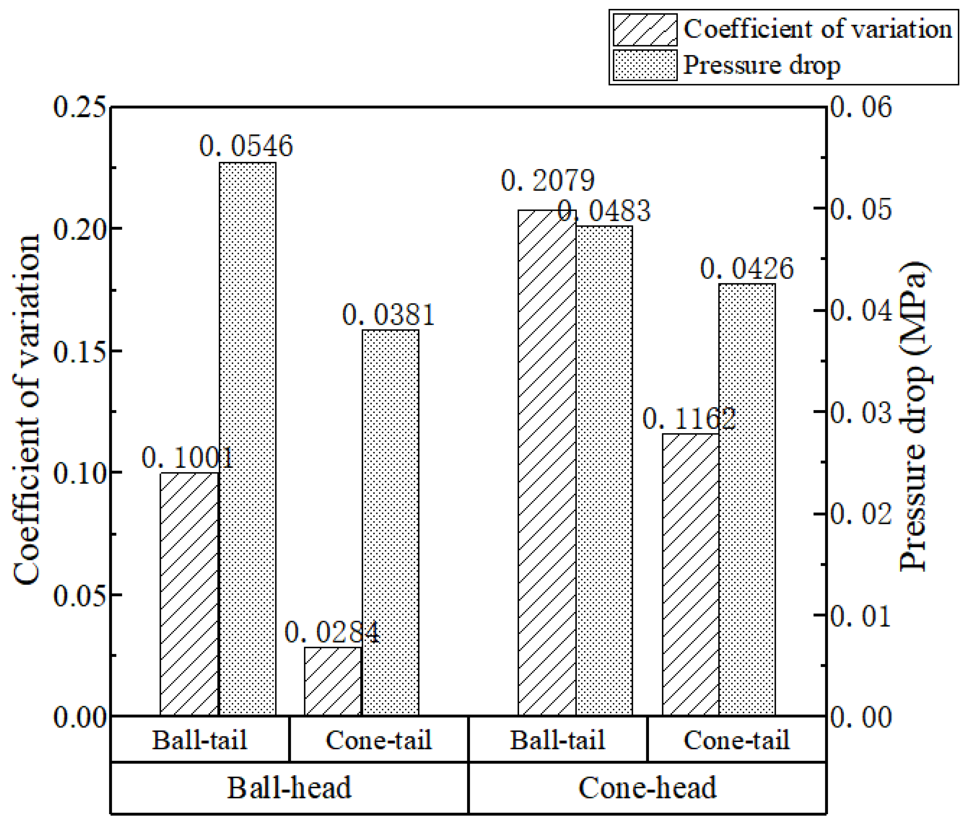
3.2.1. Influence of the Head Structure Shape on the Mixing Effect

Spherical and conical head structures were proposed for this mixer. And because the heads were divided into an inlet and an outlet, the ball-head cone-tail shape, cone-head cone-tail shape, ball-head ball-tail shape and cone-head ball-tail shape were selected in the same model for simulation and analysis to obtain the coefficient of variation characterizing the mixing uniformity of the mixer and the pressure drop distribution of energy loss, as shown in Figure 2.

As shown in Figure 2, the head structure has a significant influence on the coefficient of variation of the mixing uniformity of the mixer, with the coefficient of variation of the ball-head cone-tail structure being the smallest at 0.0284. The flow field analysis shows that the ball-head at the inlet can ensure the integrity of the internal flow field and reduce structural distortion while forming a certain diffusion effect of the flow field, thus accelerating the formation of turbulence and promoting mixing. The cone-tail at the outlet can produce a contraction effect of the flow field, increasing the outlet flow rate and achieving further mixing of the pesticide and water. Moreover, considering the pressure loss caused by different structures, the influence of different heads on internal pressure loss is relatively smaller. Hence, the optimal head structure for the mixer is the ball-head cone-tail shape.

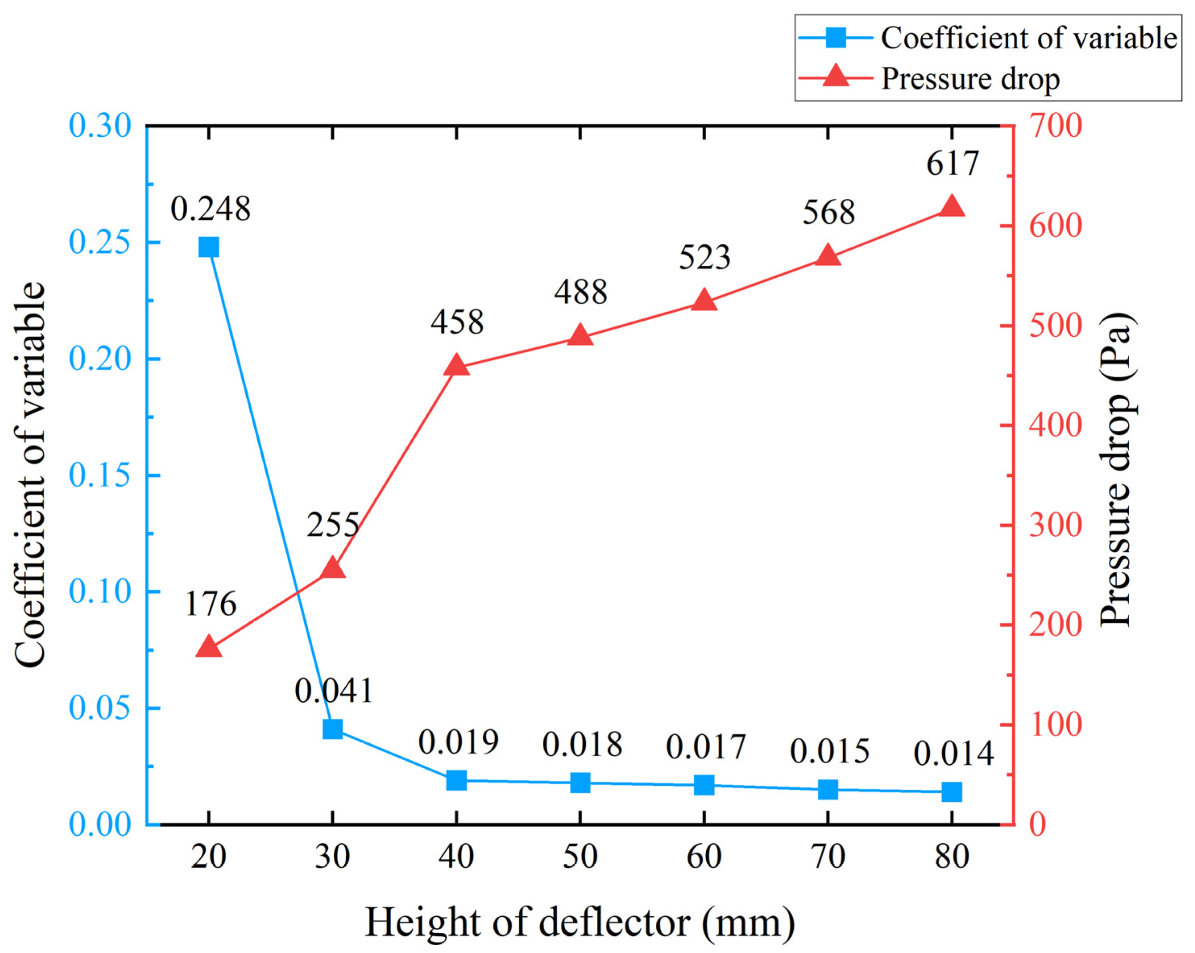
3.2.2. Influence of the Height of the Deflector on the Mixing Effect

Due to the stable structure of the semicircular baffles, the influence of height on the mixing effect was not considered, and only that of isosceles baffles was analyzed. The height of the baffle was set based on the size of the cylinder cavity. The simulation and comparison test of the isosceles baffle with 7 kinds of heights, 20 mm, 30 mm, 40 mm, 50 mm, 60 mm, 70 mm and 80 mm, were carried out based on the ball-head cone-tail mixer, and the mixing performance of the baffle was analyzed. The coefficient of variation, which characterized the mixing uniformity of the mixer, and the pressure drop distribution of the energy loss are shown in Figure 3.

As shown in Figure 3, the height of the isosceles baffle has a great influence on the mixing performance of the mixer. With increases in the height of the baffle, the coefficient of variation of mixing decreases obviously. However, as the height of the deflector increases, the corresponding internal pressure loss also increases significantly. This is because a very high deflector setting has an obvious obstructive effect on the fluid inside the mixer, and while it enhances the mixing effect, the power consumption of the liquid flow is also significantly increased. Therefore, in terms of the isosceles baffle, a relatively moderate height of the baffle was selected after comprehensive consideration: that is, the height does not exceed the radius value of the cylindrical main pipe. The height of the baffle was selected as 50 mm, which is consistent with the semicircular baffle.

3.2.3. Influence of the Angle of the Deflector on the Mixing Effect

Also, because the structure of the semicircular baffle was stable, the influence of the angle on the mixing effect was not considered, and only that of the isosceles baffle was analyzed. The setting of the deflector angle had a great influence on the formation of the internal flow field. Based on the ball-head cone-tail mixer whose height of the isosceles deflector was 50 mm, five angles of 30°, 60°, 90°, 120° and 150° were selected for comparative analysis to determine the optimal angle-setting parameters for the deflector. The coefficient of variation characterizing the mixing uniformity of the mixer and the pressure drop distribution of the energy loss are shown in Figure 4.

As shown in Figure 4, the layout angle of the isosceles baffle has a great influence on the mixing performance of the mixer. As the deflector angle increases, the first half of the coefficient of variation becomes relatively stable, and the coefficient of variation of the mixing uniformity is optimal when the deflector is 90°. Beyond 120°, the coefficient of variation increases significantly, indicating that the disturbance effect on the internal flow field of the mixer is significantly reduced after the deflector is arranged beyond this angle. In addition, with an increase in the angle of the deflector arrangement, the corresponding internal pressure loss decreases. However, the pressure drop increases when the angle exceeds 120°, indicating that the obstructive effect of the deflector on the internal fluid of the mixer gradually strengthens again beyond this angle and the energy loss gradually increases. Therefore, the mixing effect of the mixer is optimal when the angle of the isosceles baffle is set to 90°.

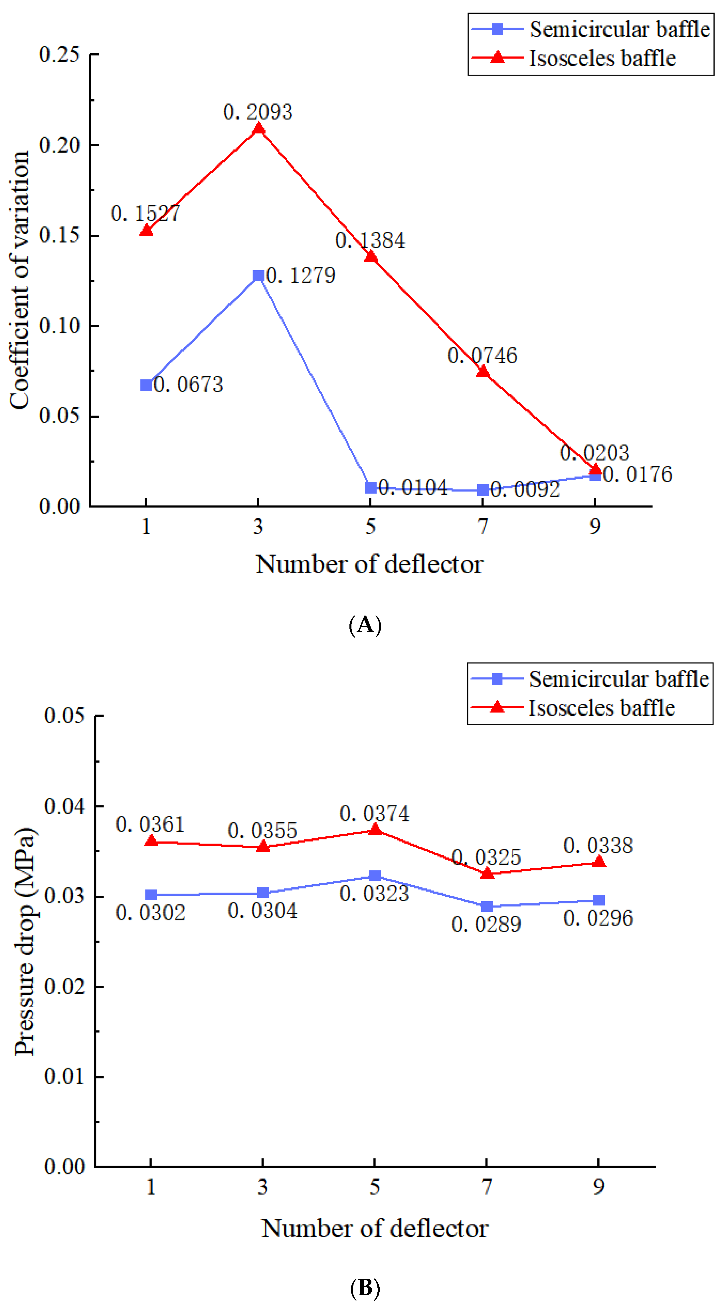
3.2.4. Influence of the Structure and Number of Deflectors on the Mixing Effect

The influence of the baffle structure on the mixing performance of the mixer was also analyzed through the combination and comparison of single-factor analysis. According to the design basis of the industrial mixer and the characteristics of the flow field, it was more appropriate to set the number of baffle plates as odd [34]. Based on the ball-head cone-tail mixer with an optimal baffle structure, the numbers of 1, 3, 5, 7 and 9 baffles were selected for comparative analysis in this paper; the coefficient of variation of the mixing uniformity and pressure drop distribution of the mixer for different structures and numbers of deflectors are shown in Figure 5.

By comparing and analyzing the influence of the deflector plate structure on the mixing performance of the mixer, it can be observed from Figure 5A that the coefficient of variation of the mixing with semicircular deflector plates is generally better than that with isosceles structures and that the more deflectors are considered, the better the mixing uniformity is. Analysis of Figure 5B reveals that the deflector plate setting has no significant effect on the overall internal pressure loss. As shown in Figure 5, the minimum coefficient of variation and pressure drop are observed to be smallest when the number of semicircular deflectors is set to seven. Therefore, it is optimal to arrange seven semicircular baffles in the inner cavity of the mixer.

3.2.5. Effect of Changes in Mixing Ratio on the Mixing Effect

According to the requirements of the assignment book of related funded projects and the agronomic requirements of related plant protection operations, the mixer studied in this paper and its matched mixing system should be able to work stably within the range of mixing ratios from 300:1 to 3000:1, and the mixing coefficient of variation of the mixer should meet the task requirements [35]. On this basis, this study investigated the mixing performance of a ball-head cone-tail mixer according to the changes in the mixing ratio. When considering the changes in the mixing ratio, the relevant structural parameters of the mixer adopted the previous optimal structure; that is, the head adopted the ball-head cone-tail structure, the number of internal deflector plates was seven, the deflector plates adopted a semicircular structure and the angle of the deflector plates was set at 90° for the simulation. In the simulation process, the mixing ratios were 300:1, 600:1, 900:1, 1200:1, 1500:1, 2000:1, 2500:1 and 3000:1. The cross-sections were taken at 110 mm, 210 mm, 310 mm, 410 mm, 510 mm, 610 mm and 690 mm in the axial direction of the mixer, and the distribution volume fraction of pesticides at each section position was calculated. Therefore, the distribution of variation coefficient of potion mixture in the simulation process was obtained, as shown in

Table 3. Simulation coefficient of variation of selected cross-section positions under various mixing ratios.

Mixture Ratio	Coefficient of Variation of Each Axial Cross-Section Position of the Pesticide Mixer
	110 mm	210 mm	310 mm	410 mm	510 mm	610 mm	690 mm
300:1	26.11%	11.24%	5.58%	4.01%	3.15%	3.11%	2.22%
600:1	26.74%	11.28%	5.24%	3.51%	2.91%	2.90%	2.88%
900:1	26.85%	11.37%	5.05%	3.28%	2.88%	2.84%	2.63%
1200:1	26.82%	11.53%	5.21%	3.38%	2.85%	3.33%	2.55%
1500:1	27.39%	11.43%	5.01%	3.29%	2.77%	3.35%	2.34%
2000:1	27.26%	11.49%	5.33%	3.34%	2.78%	3.29%	2.38%
2500:1	25.44%	10.70%	5.27%	4.01%	2.83%	3.12%	2.54%
3000:1	25.31%	10.77%	5.31%	4.05%	3.35%	2.99%	2.44%

.

The results in Table 3 indicate that the overall mixing coefficient of variation of the ball-head cone-tail mixer is improved with the changes in mixing ratio, with an optimal mixing effect observed at the ratio of 300:1, where the coefficient of variation is 2.22%. The coefficient of variation in the simulation is approximately 5% for all mixing ratios with a cross-section of 310 mm, indicating that the mixer has achieved uniform mixing halfway along the axial direction inside the mixer. At the mixing ratio of 3000:1, the coefficient of variation for a cross-section of 690 mm is 2.44%, which meets the requirement of a coefficient of variation of less than 5%. The simulation results show that the mixer can achieve good mixing at ratios ranging from 300:1 to 3000:1 with a ball-head cone-tail structure and seven deflector plates of a semicircular structure, which meets the requirements of design.

4. Mixing Uniformity Test

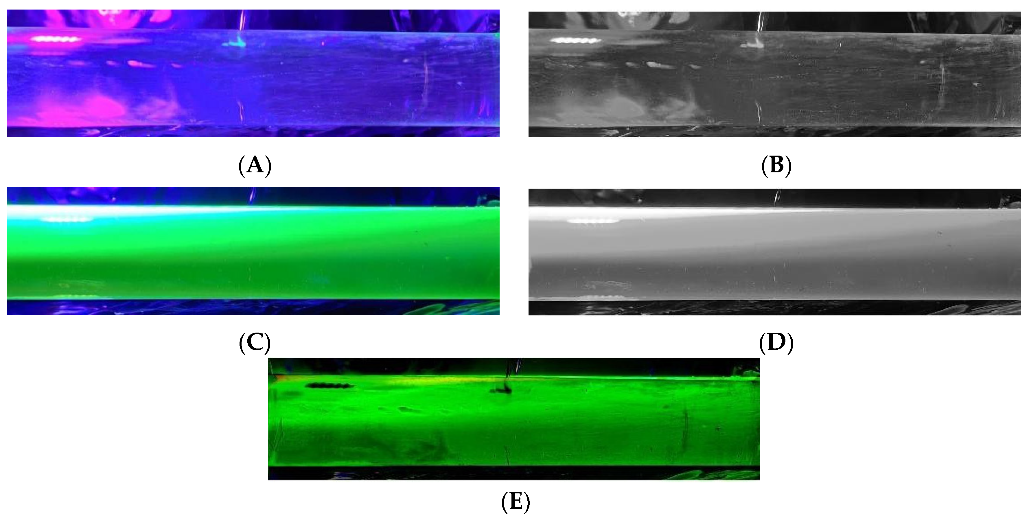
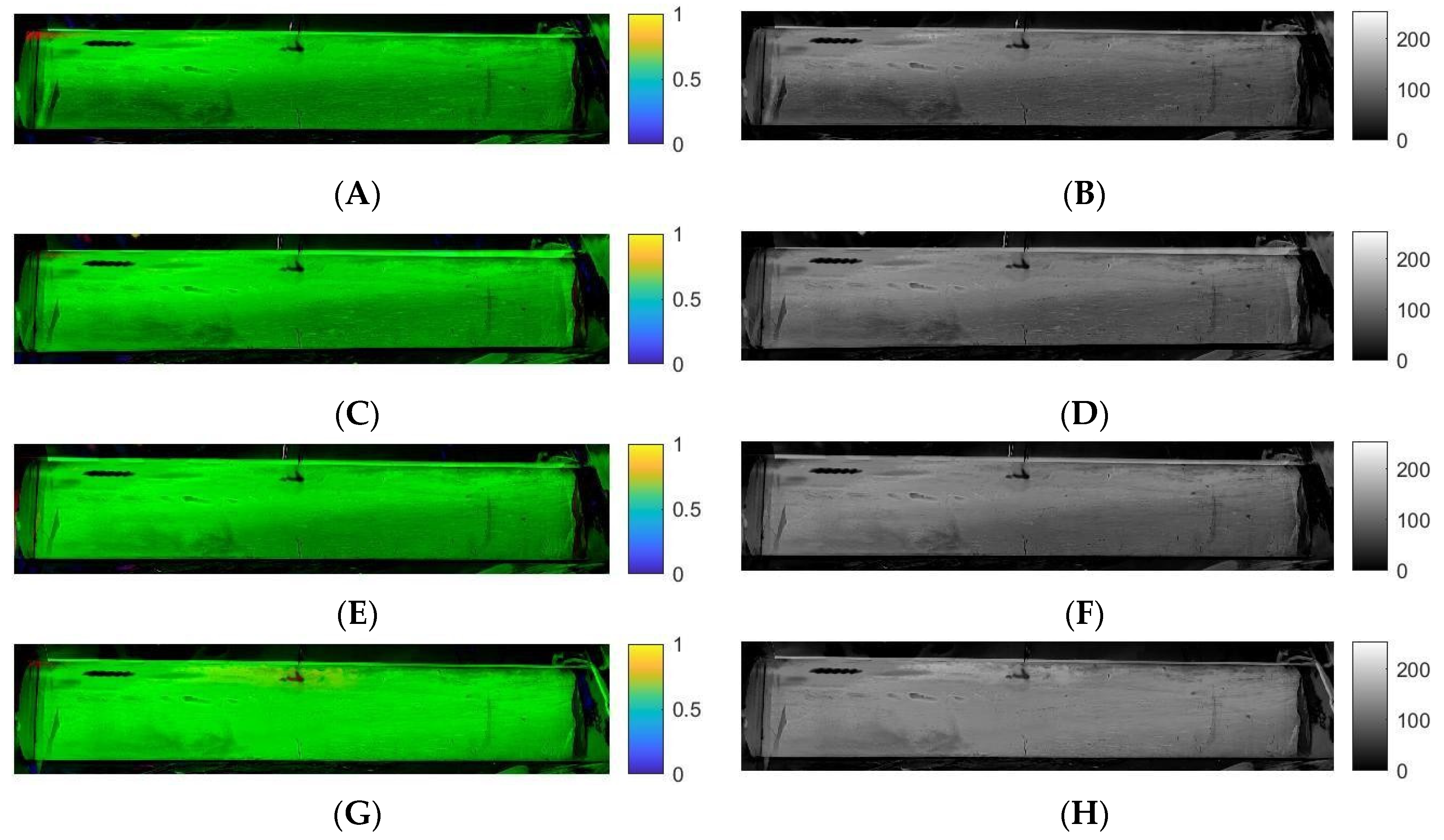
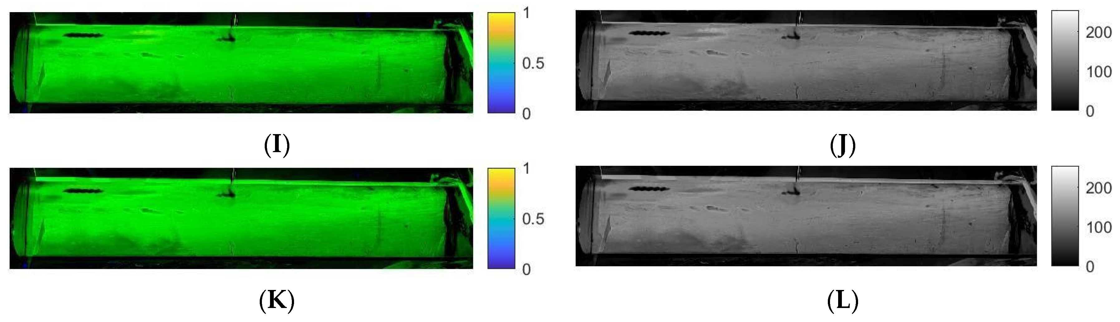
4.1. Qualitative Analysis of Mixing Uniformity of Ball-Head Cone-Tail Mixer

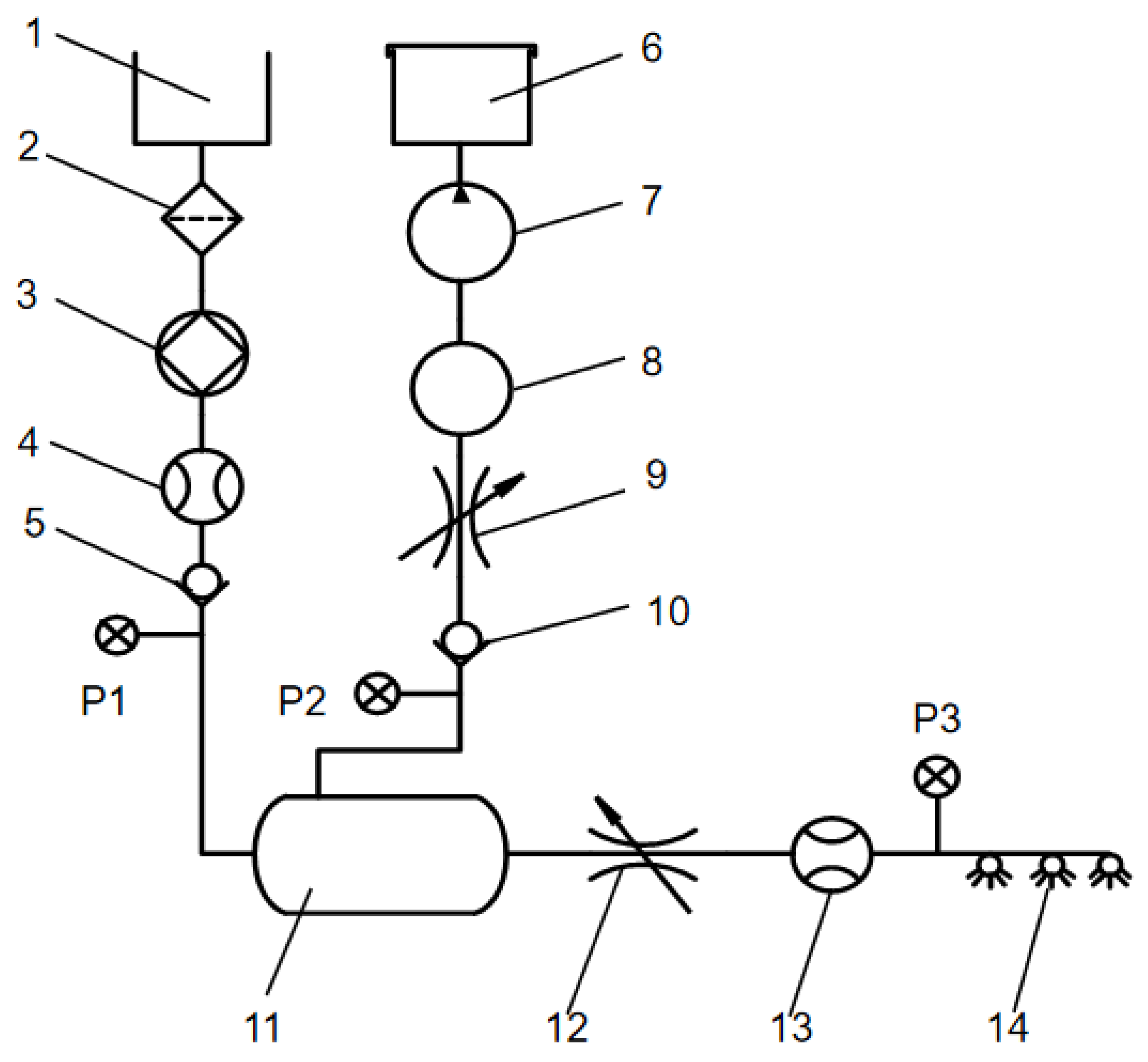
4.1.1. Test Conditions

The mixer was manufactured according to the optimal structural parameters, and the ball-head cone-tail mixer and its matched mixing system (as shown in Figure 6) were verified by laboratory tests. Considering that a series of stratification phenomena often occur in the mixing process of pesticides, the mixing performance of the mixer was qualitatively analyzed using the image analysis method of high-definition photography, and the mixing performance of the mixer was quantitatively analyzed from the aspect of spatial and temporal distribution uniformity under different proportions.

The qualitative test table of the mixing system is shown in Figure 7. HD photography mainly includes two parts, among which the hardware part contains an HD camera, mobile light source, image acquisition card and mobile workstation. This part is mainly used to photograph the mixing of the pesticide in the delivery process. In order to ensure the authenticity of the shot image, the mobile light source is a domestic LED purple lamp with a power of 50 w. The wavelength of this light can perfectly combine with the fluorescent particles in the aqueous solution. According to the luminescence in the aqueous solution, the image taken by the high-definition camera can be analyzed so that the experimental results can be obtained. The image integration card is Camware3, a software of Pco company, which can control the camera according to different working conditions. It can also adjust the number of frames taken and display a time scale on each frame. It has comprehensive functions and can process and save the images taken to meet the test requirements.

The test adopts the peristaltic pump to extract the liquid. Considering that the speed of the peristaltic pump is too fast, the liquid velocity will be unstable, the liquid can not flow normally when the speed is too small, and the pesticide can not enter the mixer normally. Therefore, in order to prevent the liquid from flowing unnormally in the process of mixing at a relatively ratio, the booster pump is used to properly pressurize during the test, which can reduce the impact of pressure loss. The pressure of the booster pump is 1 MPa, the maximum working flow is 7 L·min⁻¹, and the voltage is DV 24 V. The booster pump is installed at the outlet end of the peristaltic pump, and the pesticide stock liquid transported by the peristaltic pump is pressurized and transported through the booster pump. At the same time, the throttle valve is connected at one end of the booster pump to avoid the booster pump from drawing water from the aqueous solution.

Considering the actual processing and equipment, the mixer is made of stainless steel welded as a whole, and a section of plexiglass observation tube is designed at its outlet for the image analysis test.

4.1.2. Area Calibration of the Mixer Observation Tube

The images captured by the HD camera system used in the experiment are the qualitative analysis of the mixing performance test of the mixing system. Since this experiment mainly tests the mixing conditions of pesticides in the mixer, the images taken by the HD camera need to be further processed to find the appropriate images, as shown in Figure 8:

Before the test, it is necessary to shoot and calibrate mixed and aqueous solutions of pesticides in advance. The specific methods are as follows:

In order to ensure that the image taken was more clear, a phosphor solution, which was calibrated and prepared in advance, was used for qualitative tests instead of common water-soluble pesticides. The optical property of fluorescent powder was applied to amplify the distribution characteristics of alternative pesticides for the acquisition of image materials. The image subtraction was carried out on the original image materials to eliminate the interference of the image background and other factors. The region of interest was set as shown in Figure 9. The 250 × 600 pixel area was used in the experiment; then, the image was binarized, and a threshold value of 0.2 was selected as the standard. If the threshold was exceeded, it was marked as 1, indicating the presence of fluorescent particles. According to Formula (4), further programming processing was carried out in the software, and image materials under the corresponding concentration ratio obtained by the experiment were selected and analyzed. In addition, the pictures were drawn according to the actual experimental results, and the axial and radial grayscale values of the region of interest were counted to find the distribution regulation. In the process of picture collection, pictures of pesticide solutions with different concentration ratios were selected. The collected pictures needed to be preprocessed before processing, and the grayscale values of the images needed to be inputted after the regions of interest were divided. Finally, the collected image data were drawn into the pictures, and the mixing of pesticides was analyzed.

$$\mathrm{y}=\frac{\mathrm{s}-{\mathrm{s}}_1}{\mathrm{s}}\times 100\%,$$

(4)

Note: $\mathrm{s}$, total area; ${\mathrm{s}}_1$, threshold < 0.2 region; $\mathrm{y}$, the proportion of pesticide regions.

4.1.3. RMSE Analysis

Appropriate regions of interest were selected for observation according to the fixed mixing ratio in the tube. The regions of interest used in the experiment were w = 80 and h = 60. Analysis results of the root mean square error are shown in Figure 10.

Figure 10A is the grayscale value distribution of the observed region of interest. It can be clearly seen from the figure that the grayscale value distribution is relatively uniform and no variation occurs. In addition, it can be seen from the figure that the selected observation area is the area with the largest inner diameter of the cylindrical observation tube and the area with the largest relative wall thickness and mixed solution, so the grayscale distribution in the middle part of the figure is more concentrated than that on both sides. In addition, the grayscale distribution of the upper part is slightly increased compared with that of the lower part. This phenomenon is because the supplementary light source for photography is installed on the left of the upper part of the observation tube, and the grayscale distribution of the light source is slightly affected. Figure 10B shows the calculated root mean square error value of 6.2868, which is relatively small, so it can be recognized that the internal mixed solution has good uniformity.

According to the same test method, the mixing conditions of different mixing ratios within the range of 1:600–1:3000 were analyzed and treated, respectively, and the treatment results are shown in Figure 11.

In order to reduce the influence of other pixels on the analysis results, the original color image was grayscale processed to obtain the grayscale processed image at the corresponding proportion, respectively, and the calibration diagram of pure water was subtracted from each image to obtain the distribution diagram of the corresponding grayscale value. At the same time, the distribution of pesticides and water at different proportions was finally obtained by referring to the above method, as shown in Figure 12.

From the above distribution images, it can be seen that a small amount of grayscale distortion exists locally in the observation area within the mixing ratio range of 1:3000–1:30,000. This situation is possibly because the pesticide may be distributed in a flocculent form in some cases, and it is not fully mixed with water in time. The overall gray distribution is relatively uniform, which indicates that the distribution of pesticides and water is relatively uniform in the macro view under different mixing ratios.

4.2. Quantitative Analysis of Mixing Uniformity of Ball-Head Cone-Tail Mixer

4.2.1. Test Methods and Calibration

By referring to the relevant literature [26,36,37,38,39,40] and combining it with the existing conditions in the laboratory, UV spectrophotometry was used to quantitatively detect the mixed solution of the mixer. The UV spectrophotometer used in this test was a Shimadzu UVmini-1240. To further verify the reliability of the test, a quantitative test was performed by proportionally preparing a carmine solution instead of water-soluble pesticides. The absorbance was calibrated based on different concentrations of the carmine solution. A solution with a concentration of 3 g·L⁻¹ was prepared as a dilution stock solution, and a reference mixture at the corresponding mixing ratio of 300:1 to 3000:1 was obtained, in addition to a sample of pure water as a reference. The absorption wavelength of the spectrophotometer was set at 507 nm [41], the absorbance of samples were tested, and the averages of the measurements were taken as the data for the experiments, as shown in

Table 4. Absorbance data for diluted samples.

Sample Number	Concentration (mg·L−1)	Absorbance
1	1	0.022
2	1.5	0.033
3	2	0.041
4	2.5	0.053
5	3	0.066

.

By usingthe MATLAB software, the obtained experimental data were processed and expressed in a regression equation, which was specifically calculated as

$$\mathrm{ABS}=0.0216\mathrm{C}-0.0002,$$

(5)

where $\mathrm{ABS}$ denotes the absorbance and $\mathrm{C}$ denotes the concentration (mg·L⁻¹).

During the test, the water flow was set as the maximum flow required by design to supply the corresponding mixing ratio. The specific test methods were mainly as follows:

(1)

Sampling from the outlet of the mixer for 2 s at 30 s intervals to obtain 5 samples of the mixture at different times.

(2)

Sampling ten points at different spatial locations between the outlet end of the mixer and the nozzle and each for 2 s.

The absorbance of the sampled solutions was compared to analyze the mixing time and spatial homogeneity of the ball-head cone-tail injection mixer. Figure 13 shows the quantitative test table of the online mixing system for mixing uniformity.

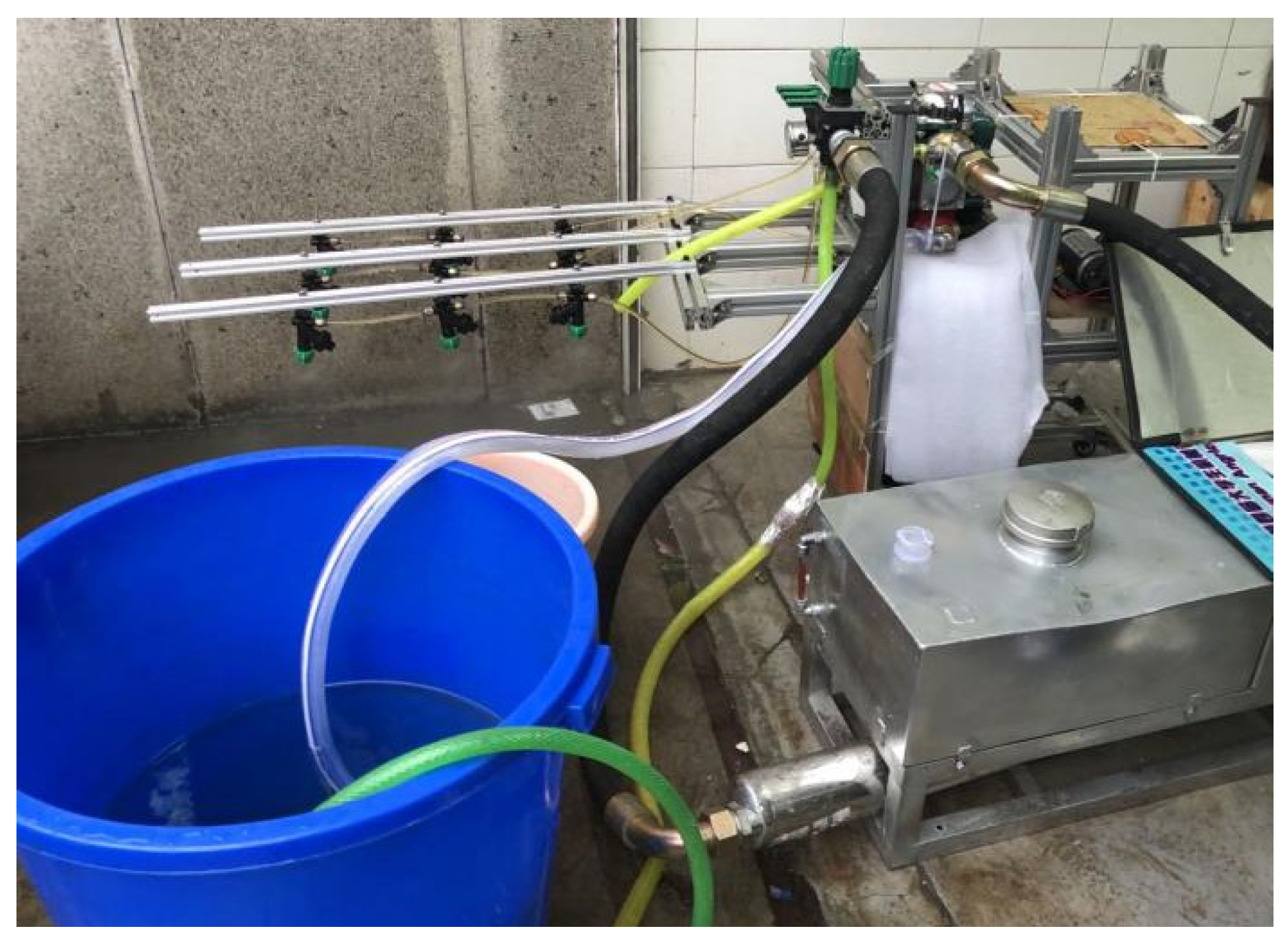
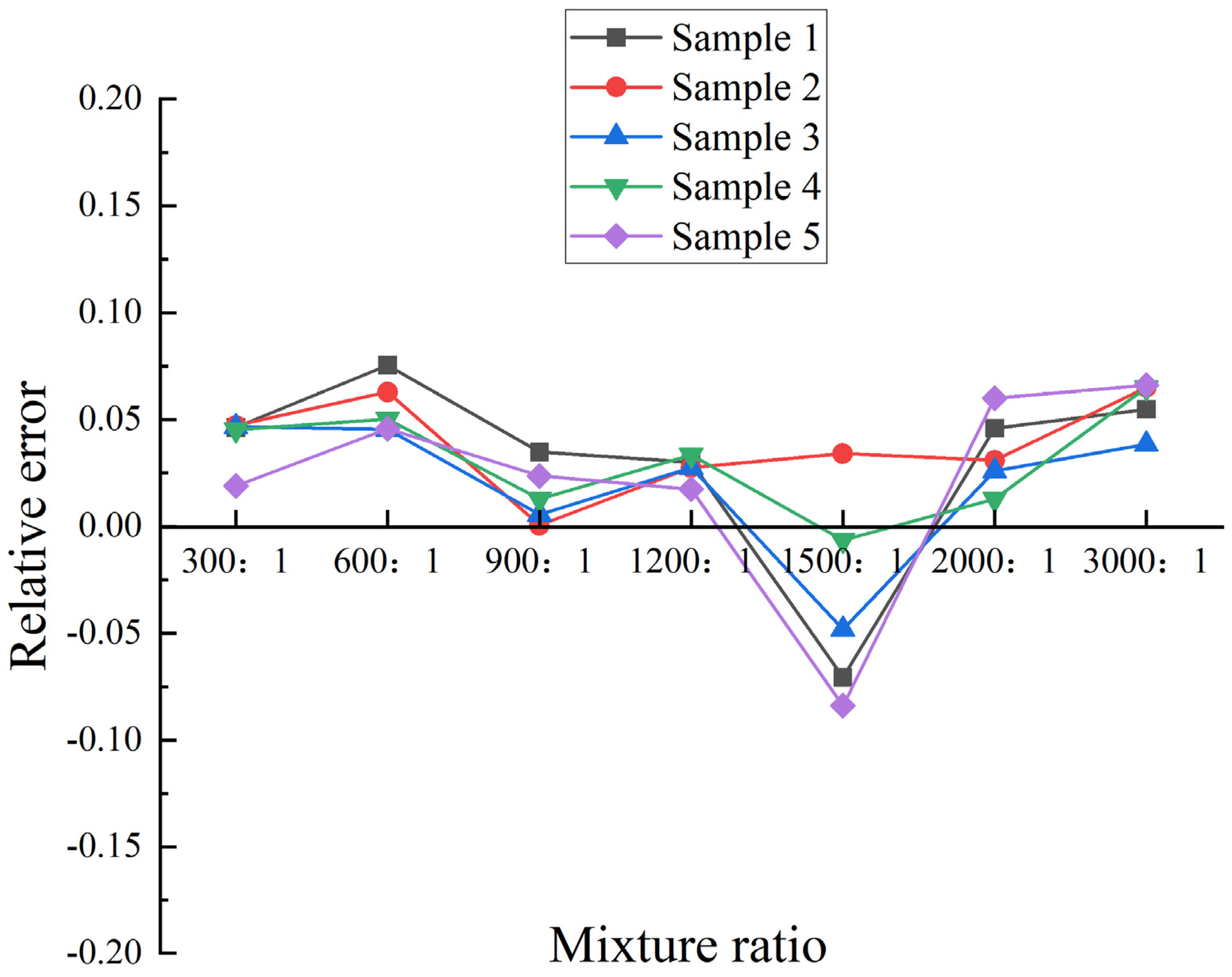
4.2.2. Temporal Distribution Uniformity Test

On the pressurized experimental table, the mixing ratio was changed, and samples were taken 5 times at the outlet of the mixer according to the test scheme (1). After sampling, samples were placed in the spectrophotometer for real-time detection, and sample concentrations under different mixing ratios were obtained, as shown in

Table 5. Sample concentrations at different times and various mixing ratios.

Mixture Ratio	Sample 1	Sample 2	Sample 3	Sample 4	Sample 5	Expected Concentration
300:1	9.557	9.549	9.555	9.568	9.814	10
600:1	4.649	4.704	4.783	4.761	4.781	5
900:1	3.218	3.328	3.311	3.288	3.253	3.33
1200:1	2.427	2.433	2.433	2.419	2.457	2.5
1500:1	2.152	1.934	2.101	2.013	2.183	2
2000:1	1.434	1.455	1.462	1.481	1.415	1.5
3000:1	0.948	0.939	0.963	0.939	0.938	1

(unit: mg/L). The line diagram of the relative error of sample concentrations is shown in Figure 14.

Table 5 shows that the actual concentration of the mixture collected by the ball-head cone-tail mixer is similar to the expected concentration, indicating that the mixture is uniform. From the data in the table, it can be found that the concentration values of the solutions sampled at multiple intervals at the same mixing ratio have a small error, indicating that the mixing performance of the ball-head cone-tail mixer is stable in continuous operation and that its time distribution is uniform. The actual concentrations of the sample solutions are both higher and lower compared to the expected concentrations because the pesticide and water do not achieve 100% full mixing, with some solutions having a pesticide content lower than expected and some solutions having a pesticide content higher than expected. As shown in Figure 14, the relative error indicated from the mixing performance of the mixer is stable when the mixing ratio is changed, essentially not exceeding the relative error value of 0.08. This result is consistent with the simulation results. And the structure of the ball-head cone-tail mixer is optimized at the inlet and outlet sections, its port apertures are arranged in accordance with the requirements of the installation, and the ball-head cone-tail mixer has a stable temporal distribution uniformity under continuous operation.

4.2.3. Spatial Uniformity Test

The mixing ratio was varied according to test protocol (2) and samples were collected at 10 different locations with the expected concentrations consistent with the above temporal uniformity test. The sample concentrations at different mixing ratios were obtained after being tested as shown in

Table 6. Sample concentrations at different spatial locations and various mixing ratios.

Sample Point	Sample Concentration at Various Mixing Ratios (mg·L−1)
	300:1	600:1	900:1	1200:1	1500:1	2000:1	3000:1
1	9.541	4.681	3.094	2.388	1.912	1.417	0.918
2	9.544	4.683	3.095	2.389	1.914	1.418	0.920
3	9.543	4.682	3.094	2.388	1.913	1.417	0.919
4	9.544	4.683	3.095	2.389	1.914	1.418	0.918
5	9.544	4.683	3.095	2.389	1.914	1.418	0.920
6	9.543	4.682	3.094	2.388	1.913	1.417	0.919
7	9.543	4.682	3.094	2.388	1.913	1.417	0.919
8	9.543	4.682	3.094	2.388	1.913	1.417	0.919
9	9.544	4.683	3.095	2.389	1.914	1.418	0.918
10	9.544	4.683	3.095	2.389	1.914	1.418	0.918

. The relative errors of sample concentrations are shown in Figure 15.

The data presented in Table 6 show the actual mass concentrations at the selected sampling points corresponding to the different mixing ratios. Figure 15 shows that the relative error of the concentration at each spatial position under the same mixing ratio is stable. The table and the figure reflect that the actual concentration of the solution, which comes from the mixer, flows through the water distributor and is transported through the spray bar, remains stable, indicating that the mixing of the pesticide and water has been completed in the mixer and that the subsequent transport process has little impact on its concentration.

5. Conclusions

A new type of injection mixer was designed and numerically simulated using CFD. The main component of the mixer was cylindrical. The head structure and the shape, number, height and angle of the mixer deflector were compared and analyzed. The optimal head structure was determined to be the ball-head cone tail shape. The deflector plate was shaped as a semicircle at an angle of 90°, and the best mixing performance was achieved with the number of seven. At mixing ratios of 300:1–3000:1, the mixing coefficient of variation was within 5%, satisfying the design requirements.

The mixing performance of the mixer was analyzed qualitatively and quantitatively through experiments. When the pressure was 1 MPa, the distribution uniformity of the pesticide and water under different mixing ratios was analyzed using the image analysis method of high-definition photography. The spatial and temporal uniformity of mixing was verified using ultraviolet spectrophotometry on the ball-head cone-tail mixer. The grayscale distribution of the solution under different mixing ratios in the mixer is uniform, indicating that the distribution of pesticide and water in the solution is uniform and the mixing effect is good. The sampling error at multiple intervals of the mixer is small, which indicates that the time distribution uniformity is relatively great on the whole. The mass concentration of the mixture at different locations changes little, indicating that the spatial distribution uniformity of the mixer is good.

The mixer designed in this paper solves the problem that the ratio of pesticide and water in existing mixers is relatively small and unadjustable and realizes the goal of active mixing with a large ratio, which is of great significance for pesticide spraying with a precise reduction in plant protection operations, and also provides a reference for the subsequent realization of accurate online variable spraying technology. However, in this paper a carmine aqueous solution was used to replace pesticides in the test, and whether real pesticides can be mixed uniformly when mixed with water in the mixer needs to be further verified through experiments. In addition, the mixer designed in this paper only takes water-soluble pesticides as the mixing target at present, and the mixing of other kinds of pesticides, such as powder and fat soluble pesticides, will also become the focus of subsequent research in this paper.

References

1. He, X. Research progress and developmental recommendations on precision spraying technology and equipment in China. Smart Agric. 2020, 2, 133–146. [Google Scholar]
2. Tudi, M.; Daniel, R.H.; Wang, L.; Lyu, J.; Sadler, R.; Connell, D.; Chu, C.; Phung, D.T. Agriculture Development, Pesticide Application and Its Impact on the Environment. Int. J. Environ. Res. Public Health 2021, 18, 1112. [Google Scholar] [CrossRef] [PubMed]
3. Ki-Hyun, K.; Ehsanul, K.; Shamin, A.J. Exposure to pesticides and the associated human health effects. Sci. Total Environ. 2017, 575, 525–535. [Google Scholar]
4. Sun, M.; Gu, S.; Kong, D.; Hui, X.; Sun, Z. The existing problems of pesticide use and the countermeasures. J. North. Agric. 2004, 50, 141–143. [Google Scholar]
5. He, X.; Yan, J.; Wang, Y. T-shaped micromixer with periodic baffles. Opt. Precis. Eng. 2015, 23, 2877–2886. [Google Scholar]
6. He, P.; Wu, C.; Chen, C.; Wang, G.; Li, X. Performance of a new type spraying mixing apparatus. Trans. Chin. Soc. Agric. Mach. 2001, 3, 44–47. [Google Scholar]
7. Yu, Y.; Wu, J.; Meng, H. Numerical simulation process aspects of the novel static circulating jet mixer. Can. J. Chem. Eng. 2011, 89, 460–468. [Google Scholar] [CrossRef]
8. Fang, K.; Qiu, W.; Zhou, L. Design of jet mixer based on theoretical model and CFD assistance. J. Chin. Agric. Mech. 2023, 44, 65–70. [Google Scholar]
9. Zhou, L.; Fu, X.; Xue, X.; Zhou, L.; Kong, W.; Qiu, W. Design and experiment of jet mixing apparatus based on CFD. Trans. Chin. Soc. Agric. Mach. 2013, 44, 107–112. [Google Scholar]
10. Qi, H.; Liao, H.; Lan, Y. Research status and prospect of automatic pesticide mixing device. J. Agric. Sci. Technol. 2019, 21, 10–18. [Google Scholar]
11. Shi, Y.; Jiang, P.; Xiang, S.; Zhai, S. Design and optimization analysis of multi-source inmixer based on CFD. Agric. Eng. Equip. 2022, 49, 6–10. [Google Scholar]
12. Liu, T.; Ma, Y.; Yang, W.; Ji, W.; Wang, R.; Jiang, P. Spatial-temporal interaction learning based two-stream network for action recognition. Inf. Sci. 2022, 606, 864–876. [Google Scholar] [CrossRef]
13. Eakarach, B. A review on numerical consideration for computational fluid dynamics modeling of jet mixing tanks. Korean J. Chem. Eng. 2016, 33, 3050–3068. [Google Scholar]
14. Song, Y.; Lei, Z.; Lu, X.; Xu, G.; Zhu, J. Optimization of a Lobed Mixer with BP Neural Network and Genetic Algorithm. J. Therm. Sci. 2023, 32, 387–400. [Google Scholar] [CrossRef]
15. Wu, Z.; Fan, D.; Zhou, Y.; Li, R.; Noack, B.R. Jet mixing optimization using machine learning control. Exp. Fluids 2018, 59, 131. [Google Scholar] [CrossRef] [Green Version]
16. Li, Y.; Wu, S.; Liu, Y.; Wang, N.; Dai, P.; Yang, Q.; Lu, H. The coupled mixing action of the jet mixer and swirl mixer: An novel static micromixer. Chem. Eng. Res. Des. 2022, 177, 283–290. [Google Scholar] [CrossRef]
17. Sun, D.; Liu, W.; Li, Z.; Zhan, X.; Dai, Q.; Xue, X.; Song, S. Numerical Experiment and Optimized Design of Pipeline Spraying On-Line Pesticide Mixing Apparatus Based on CFD Orthogonal Experiment. Agronomy 2022, 12, 1059. [Google Scholar] [CrossRef]
18. Song, H.; Xu, Y.; Zheng, J.; Dai, X. Structural parameters optimization of swirling jet mixer based on reducing effective length. Trans. Chin. Soc. Agric. Eng. 2018, 34, 62–69. [Google Scholar]
19. Song, H.; Xu, Y.; Zheng, J.; Wang, X.; Zhang, M. Structural analysis and mixing uniformity experiments of swirling jet mixer for applying fat-soluble pesticides. Editor. Off. Trans. Chin. Soc. Agric. Eng. 2016, 32, 86–92. [Google Scholar]
20. Zhao, S.; Sheng, L.; He, W.; Zhu, N.; Li, Y.; Ji, D.; Guo, K. Design and optimization of a novel ellipsoidal baffle mixer with high mixing efficiency and low pressure drop. J. Chem. Technol. Biotechnol. 2022, 97, 3121–3131. [Google Scholar] [CrossRef]
21. Mahmoodi, H.; Razzaghi, K.; Shahraki, F. Improving mixing performance by curved-blade static mixer. AIChE J. 2020, 66, e17034. [Google Scholar] [CrossRef]
22. Xu, Y.; Wang, X.; Zheng, J.; Zhou, F. Simulation and experiment on agricultural chemical mixing process for direct injection system based on CFD. Trans. Chin. Soc. Agric. Eng. 2010, 2010, 148–152. [Google Scholar]
23. Zhao, S.; Nie, Y.; Wei, Y.; Yu, P.; He, W.; Zhu, N.; Li, Y.; Ji, D.; Guo, K. Design and parametric optimization of a fan-notched baffle structure mixer for enhancement of liquid-liquid two-phase chemical process. Int. J. Chem. React. Eng. 2022, 21, 687–699. [Google Scholar] [CrossRef]
24. Shi, Y.; Jiang, P.; Wang, F.; Zhou, S. Experimental Study on Mixing Uniformity of Injection On-Line Mixer of Crop Protection Equipment. Int. J. Heat Technol. 2021, 39, 1143–1152. [Google Scholar] [CrossRef]
25. Lei, H.; Guan, X.; Sun, Y.; Yan, H. A novel design of in-line static mixer for permanganate/bisulfite process: Numerical simulations and pilot-scale testing. Water Environ. Res. 2022, 94, e10725. [Google Scholar] [CrossRef] [PubMed]
26. Chen, J.; Xu, Y. Analysis method of pesticide on-line-mixing uniformity based on principal component analysis. J. For. Eng. 2019, 4, 121–127. [Google Scholar]
27. Yi, P.; Ma, S.; Zhang, J. Application and practice of CFD numerical simulation in the teaching fluid mechanics. J. Yili Norm. Univ. (Nat. Sci. Ed.) 2022, 16, 69–76. [Google Scholar]
28. Aanjaneya, K.; Agrawal, S. Optimization of twisted-tape element static mixers for industrially relevant setups. Chem. Eng. Res. Des. 2023, 191, 426–438. [Google Scholar] [CrossRef]
29. Zhou, M.; Bai, D.; Zong, Y.; Zhao, L.; Thornock, J.N. Numerical investigation of turbulent reactive mixing in a novel coaxial jet static mixer. Chem. Eng. Process. Process Intensif. 2017, 122, 190–203. [Google Scholar] [CrossRef]
30. Soman, S.S.; Madhuranthakam, C.M. Effects of internal geometry modifications on the dispersive and distributive mixing in static mixers. Chem. Eng. Process. Process Intensif. 2017, 122, 31–43. [Google Scholar] [CrossRef]
31. Yang, J. Selection and design application of static mixer. Chem. Equip. Technol. 1999, 20, 25–29. [Google Scholar]
32. El Habet, M.A.; Ahmed, S.A.; Saleh, M.A. Thermal/hydraulic characteristics of a rectangular channel with inline/staggered perforated baffles. Int. Commun. Heat Mass Transf. 2021, 128, 105591. [Google Scholar] [CrossRef]
33. Zhang, K. Fluent Technology Foundation and Application Examples; Tsinghua University Press: Beijing, China, 2010. [Google Scholar]
34. Heiszwolf, J.; Nyssen, O. Improving dry sorbent injection with computational fluid dynamics. NPT Procestechnol. 2016, 1, 12–13. [Google Scholar]
35. Alexey, K.; Vladimir, K.; Alexey, C.; Vyacheslav, T. Modelling the effect of continuous mixer operating parameters on mixture quality. E3S Web Conf. 2020, 164, 08009. [Google Scholar]
36. Zhao, X.; Xu, J. Design and implementation of ultra-micro nucleic acid protein analyzer. Chin. J. Med. Instrum. 2020, 44, 403–408. [Google Scholar]
37. Wang, S.; Zhang, T.; Zhao, Q.; Lyu, C. Settling performance of new type mixer-settler. J. Northeast. Univ. (Nat. Sci.) 2014, 35, 548–550. [Google Scholar]
38. Kimthet, C.; Wahyudiono; Hideki, K.; Shin-Ichro, K.; Motonobu, G. Micronization of curcumin with biodegradable polymer by supercritical anti-solvent using micro swirl mixer. Front. Chem. Sci. Eng. 2018, 12, 184–193. [Google Scholar]
39. Pourahadi, A.; Farahani, A.; Hosseiny, D.S.S.; Nojavan, S.; Tashakori, C. Developing a miniaturized setup for in-tube simultaneous determination of three alkaloids using electromembrane extraction in combination with ultraviolet spectrophotometry. J. Sep. Sci. 2019, 42, 3126–3133. [Google Scholar] [CrossRef]
40. Petit, J.; Ait-Mouheb, N.; Mas, G.S.; Metz, M.; Molle, B.; Bendoula, R. Potential of visible/near infrared spectroscopy coupled with chemometric methods for discriminating and estimating the thickness of clogging in drip-irrigation. Biosyst. Eng. 2021, 209, 246–255. [Google Scholar] [CrossRef]
41. Zeynep, K.A.; Şule, A. An Example of the Use of Spectrophotometric Method: Determining the Carmine in Various Food Products. Procedia-Soc. Behav. Sci. 2014, 116, 4622–4625. [Google Scholar]
Figure 1. The structural model of the ball-head cone-tail injection mixer and the layout of the inner flow guide plate.
Agriculture 13 01377 g001
Figure 2. Coefficient of variation and pressure drop for different head structures.
Agriculture 13 01377 g002
Figure 3. Coefficient of variation and pressure drop of different isosceles deflector heights.
Agriculture 13 01377 g003
Figure 4. Coefficient of variation and pressure drop of different isosceles deflector angles.
Agriculture 13 01377 g004
Figure 5. Mixing performance of different numbers of deflectors. (A) Coefficient of variation for different numbers of deflectors. (B) Pressure drops for different numbers of deflectors.
Agriculture 13 01377 g005
Figure 6. Structure diagram of the mixing system: 1. water tank; 2. filter; 3. plunger pump; 4. water flowmeter; 5. check valve; 6. medicine box; 7. peristaltic pump; 8. booster pump; 9. throttle valve 10. check valve; 11. mixer; 12. throttle valve; 13. liquid flowmeter; 14. nozzle. P1, P2 and P3 are pressure gauges.
Agriculture 13 01377 g006
Figure 7. Qualitative test table of online mixing system for mixing uniformity.
Agriculture 13 01377 g007
Figure 8. Image processing flow.
Agriculture 13 01377 g008
Figure 9. Observe the calibration images of pesticide and water in the tube. (A) Original drawing of pure water calibration. (B) Grayscale procession images of pure water calibration. (C) Original image drawing of pure pesticide calibration. (D) Grayscale image of pure pesticide calibration. (E) Image of pesticide solution at the ratio of 1:300.
Agriculture 13 01377 g009
Figure 10. Root mean square error analysis. (A) Grayscale distribution of interest region. (B) Analysis results of root mean square error.
Agriculture 13 01377 g010
Figure 11. RMS error analysis for 1:600–1:3000. (A) Color image of pesticide solution at 1:600 mixing ratio. (B) Grayscale processing image of pesticide solution at 1:600 mixing ratio. (C) Color image of pesticide solution at 1:900 mixing ratio. (D) Grayscale processing image of pesticide solution at 1:900 mixing ratio. (E) Color image of pesticide solution at 1:1200 mixing ratio. (F) Grayscale processing image of pesticide solution at 1:1200 mixing ratio. (G) Color imageof pesticide solution at 1:1500 mixing ratio. (H) Grayscale processing image of pesticide solution at 1:1500 mixing ratio. (I) Color image of pesticide solution at 1:2000 mixing ratio. (J) Grayscale processing image of pesticide solution at 1:2000 mixing ratio. (K) Color image of pesticide solution at 1:3000 mixing ratio. (L) Grayscale processing image of pesticide solution at 1:3000 mixing ratio.
Agriculture 13 01377 g011aAgriculture 13 01377 g011b
Figure 12. Root mean square error analysis for 1:600–1:3000. (A) Grayscale distribution of pesticide solution at 1:600 mixing ratio. (B) Grayscale distribution of pesticide solution at 1:900 mixing ratio. (C) Grayscale distribution of pesticide solution at 1:1200 mixing ratio. (D) Grayscale distribution of pesticide solution at 1:1500 mixing ratio. (E) Grayscale distribution of pesticide solution at 1:2000 mixing ratio. (F) Grayscale distribution of pesticide solution at 1:3000 mixing ratio.
Agriculture 13 01377 g012
Figure 13. Quantitative test table of online mixing system for mixing uniformity.
Agriculture 13 01377 g013
Figure 14. Relative error in concentration for samples taken at different times.
Agriculture 13 01377 g014
Figure 15. Relative error in concentration for samples taken at different spatial locations.
Agriculture 13 01377 g015