Abstract
Hardness is a critical mechanical property of grains. Accurate predictions of grain hardness play a crucial role in improving grain milling efficiency, reducing grain breakage during transportation, and selecting high-quality crops. In this study, we developed machine learning models (MLMs) to predict the hardness of Jinsui No.4 maize seeds. The input variables of the MLM were loading speed, loading depth, and different types of indenters, and the output variable was the slope of the linear segment. Using the Latin square design, 100 datasets were generated. Four different types of MLMs, a genetic algorithm (GA), support vector machine (SVM), random forest (RF), and long short-term memory network (LSTM), were used for our data analysis, respectively. The result indicated that the GA model had a high accuracy in predicting hardness values, the R2 of the GA model training set and testing set reached 0.98402 and 0.92761, respectively, while the RMSEs were 1.4308 and 2.8441, respectively. The difference between the predicted values and the actual values obtained by the model is relatively small. Furthermore, in order to investigate the relationship between hardness and morphology after compression, scanning electron microscopy was used to observe the morphology of the maize grains. The result showed that the more complex the shape of the indenter, the more obvious the destruction to the internal polysaccharides and starch in the grain, and the number of surface cracks also significantly increases. The results of this study emphasize the potential of MLMs in determining the hardness of agricultural cereal grains, leading to improved industrial processing efficiency and cost savings. Additionally, combining grain hardness prediction models with the operating mechanisms of industry machinery would provide valuable references and a basis for the parameterization of seed grain processing machinery.
1. Introduction
Maize is one of the most important food crops in the world [1]; in 2022, the global maize yield exceeded one billion tons. Maize is also an essential food ingredient in countries such as Asia, Africa, and Latin America. Due to its high content of starch and various types of glucose, maize is used extensively as a raw material for food and industrial manufacturing, presenting significant potential in the market [2]. Previous studies have shown that soft maize can generate a greater starch content through wet milling. However, hard maize is better suited for dry milling and is commonly used to make low-starch products, such as pasta and maize flour [3]. Food-grade maize specifically used for dry grinding can be used to make cereal, baked goods, beer, and other daily items. Currently, the demand for food-grade maize is expanding internationally [4]. Research has found that maize that is more suitable for dry milling often has special requirements for the hardness value of the seeds. In addition, the weight, glassiness, and screening efficiency of the maize are quality characteristics that are important in the dry milling industry [5]. Mechanized harvesting has become the predominant method. However, grain harvesting entails numerous processes, including mixing, storage, transportation, and unloading. The above processes can largely destroy the surface of the grain and even accompany the occurrence of cracks and localized fragmentation, which ultimately affect the quality of the grain. Therefore, it is essential to take reasonable and effective measures to mitigate the effects of mechanization on grain to protect its integrity [6]. In recent years, grain hardness has become a standard for market pricing and grain classification, as well as an indicator used in world trade. Endosperm hardness is the primary determinant of maize grain quality. Enhancing endosperm hardness can boost flour output and generate economic gains for the food, feed, and brewing industries; additionally, it can decrease the likelihood of grain damage during mechanized operations and improve resistance to external environmental factors [7]. In addition, the hardness of grains is closely related to their internal PIN genetic genes [8]. A deeper understanding of the genetic characteristics of grains can accelerate the process of achieving breeding optimization. Therefore, it is necessary to develop a model capable of predicting grain hardness for applications in variety breeding and industrial processing to improve grain quality, reduce raw material losses, and improve processing efficiency.
In recent years, due to the increasing demand for a greater accuracy of maize quality parameters in various terminal products, there is an urgent need for technology that can achieve rapid detection with low detection costs to meet the needs of digital products. Maize grains are generally composed of water, starch, protein, fat, and soluble sugars. Scholars have conducted research on the physical properties of maize from different perspectives, such as measuring the density and volume of maize grains using X-ray computed tomography (μCT) [9]. The protein content and grain weight have a significant impact on grain hardness. In addition, some scholars have studied the growth environment of maize and the influence of starch content on grain hardness and found that there is also a certain relationship between the content of amylose and grain hardness [10]. The hardness of maize is also related to its moisture content. Normally, the higher the moisture content, the smaller the hardness value. Currently, there is a great deal of attention paid to the testing methods for grain hardness. Traditional grain quality testing methods mainly include commonly used hardness testing methods, such as the keratinization rate method, grinding method, and single-particle hardness index method [11]. However, these methods can damage the integrity of test samples and generally target multiple test samples. The measurement process is relatively complex, the accuracy is low, and it is difficult to compare different grains horizontally, which, to some extent, limits the measurement efficiency. With the continuous development of computer technology, tomography technology, near-infrared spectroscopy, and hyperspectral imaging technology are increasingly being used for the quality inspection of agricultural products [12,13,14,15]. It has been found that most previous studies on grain hardness have combined hardness with the genetic characteristics of protein, starch, and genes in the body. Currently, near-infrared spectroscopy is the mainstream method for detecting the hardness of single grains. Near-infrared spectroscopy can reliably predict the protein content, density, and endosperm vitrification inside grains with a high accuracy [16]. Biological and infrared imaging technology can quickly and non-destructively evaluate the quality parameters of maize as well as reliably predict the protein content and density with a high accuracy. It can evaluate the hardness of different grain segments, allowing for a more accurate understanding of the correlation between grain hardness and seed composition [17]. Grain hardness and starch content are the main determining factors for the ultimate use of grains. Some scholars have successfully measured the grain hardness of wheat and maize using near-infrared spectroscopy and predicted the particle size index [18]. However, this technology has high detection costs and limited detection capabilities. At present, it is only suitable for testing the quality characteristics of small-scale grains and is not suitable for large-scale finished product testing in many processing fields, such as in industry and agriculture [19]. Zhang et al. [20] used the indentation loading curve method to measure the hardness of grains such as wheats, peas, maize, and mung beans. The results showed that this method has a high measurement accuracy and good applicability and can measure the hardness of various grains. The principle of this method is to analyze the loading curve, calculate the slope of the linear segment (SLS), and then use the virtual elastic modulus method to characterize the grain hardness [21,22]. It is more suitable for detecting the hardness information of large-scale agricultural materials. MLMs are currently a prominent area of academic research in the world. Compared to conventional regression models, MLMs exhibit remarkable benefits in terms of their data fitting capability, adaptive learning, parallel processing, and resilience [23]. Many researchers have used MLMs for crop yield prediction in the agricultural field, including for maize, wheat [24], tomato [25], etc. In addition, there are also applications of MLMs in agricultural research related to the fragmentation rate of maize grains [26], the soil nutrient content [27], forestry fertilization [28], etc. However, in the field of grain hardness research, the majority of studies using neural network models to predict grain hardness are focused on wheat grains. For instance, Zhang, et al. [29] used an ant colony algorithm to optimize the SVM for wheat hardness inversion. This indicates the feasibility of an MLM in predicting grain hardness. Similarly, Hui, et al. [30] established a radial basis function and used visible near-infrared spectroscopy to predict wheat hardness. However, relatively few studies have been conducted on the prediction of maize hardness using MLMs. This may be due to the variable shape of maize grain and the fact that hardness is strongly influenced by the internal moisture and drying method used.
From the above analysis, it can be seen that MLMs have strong advantages in research index prediction, can lower the costs of experimental research, and can improve efficiency. The purpose of this study is to measure maize hardness using the indentation loading curve method and to train experimental data through MLMs to establish an algorithm model that can accurately predict the hardness of maize grain. The design of the experiment adopted the optimal Latin hypercube design (OPTLHD) to measure the hardness of maize and compared the changes in grain microstructure before and after loading the sample. Subsequently, a regression prediction analysis based on the MLMs were carried out using loading speed (LS), loading depth (LD), and different types of indenters (DI) as input variables; additionally, the slope of the linear segment (SLS) can characterize the grain hardness as the output variable. We explore the sensitivity and predictive effect of the GA, SVM, RF, and LSTM models on the relationship between maize hardness and the input variables to explore the correlation between the three input variables and maize hardness, as well as determine the optimal maize hardness prediction model. We attempt to provide accurate and reliable maize hardness indicators for industries such as breeding, food processing, and transportation and for applications such as grain classification pricing.
2. Materials and Methods
2.1. Experiment Samples of Maize Grain
The experimental materials were derived from commercially available Jinsui No.4 naturally dried maize seeds. The weight of 1000 maize grains was 351 g. These maize grains exhibited a yellowish hue, and their morphology featured a mildly serrated form. The average length, width, and height of maize grains were 14.25 mm, 7.85 mm, and 4.09 mm, respectively (Figure 1a). The moisture content of maize grain was measured by means of hot air drying. The measuring instruments included an electronic balance (PTX-FK210S, Fuzhou Huazhi Scientific Instrument Co., Ltd, Fuzhou, China) and electric drying oven (GZX-9023MBE, Shanghai Boxun Industrial Co., Ltd. Medical Equipment Factory Shanghai, China). In order to eliminate measurement errors, 50 samples were measured for moisture content, with an average value of 36.54% being the final moisture content value. The formula for calculating the moisture content of samples is as follows:
where is the moisture content of maize grains; is the initial grain weight, g; and is the grain weight after drying, g.
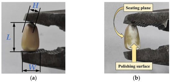
Figure 1.
Preparation of maize samples. (a) Untreated maize grain; (b) Polished maize grain.
The surface of untreated maize grains is smooth and uneven. In order to avoid lateral displacement between the grains and the contact components during the experiment, which may cause unnecessary measurement errors, it is necessary to polish the smooth surface of the maize, while the concave surface (seating plane) of the maize is not treated. The polished sample surface (the surface to be measured) should be parallel to the base surface, as shown in Figure 1b. During polishing, an electric polishing machine (S1J-SFK-003, Yonghong Strength Supplier, Jinhua, China) is used to polish the surface of 100 samples, in order to improve the stability, efficiency, and safety of the sample testing.
2.2. Design of Experiments and Methods
2.2.1. Experiment Methods
In this study, the instrument used to measure the hardness of the maize grains was the texture analyzer (TA-XT plus, Stable Micro Systems, Godalming, UK), with a maximum load of 500 N, an accuracy of 0.1 g, a force resolution of 0.0001 N, and a displacement resolution of 0.01 mm. The loading force curve and coefficient of variation can be displayed dynamically. Furthermore, the macro commands in the system allow for the direct computation and recording of desired parameters, including sample heights and curve peak points, as well as the determination of inflection points. The maize hardness measurement test consists of three main steps. Firstly, the polished maize specimen was placed horizontally on the test bench of the texture analyzer, as shown in Figure 2a. Secondly, the tip of the indenter was aligned with the center of the maize endosperm. Finally, maize hardness measurement was taken according to the combination of parameters set in the design of experiment (see Section 2.2.2). The shapes of steel needle indenters were triangular, quadrangular, conical, and spherical, respectively. All indenters had a diameter of 2 mm and a conical degree of 30°, as shown in Figure 2b.
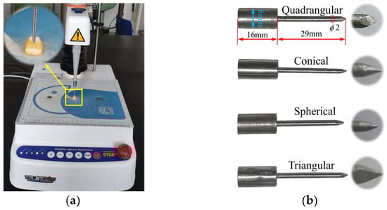
Figure 2.
Experiment apparatus and experiment processes. (a) Texture analyzer and the partial enlarged image; (b) Different types of indenters and visualization of indenter shape.
This study used the indentation loading method to determine the hardness of maize grains. The principle of this method is to use a texture analyzer to press a special shaped indenter into the maize grains and indirectly obtain the hardness of maize grains by studying the indentation (indentation depth) loading curve obtained from the experiment. We obtained a virtual elastic modulus value He that is proportional to the slope of the curve, used the virtual elastic modulus to obtain the physical meaning of He, and obtained the slope of the maize grain indentation loading curve according to a unified scaling ratio to measure the hardness information of the compressed material. The indentation loading curve and its slope comprehensively reflect the changes in indentation depth and applied load during the test process. The indentation loading curve obtained from the experiment is shown in Figure 3. This method can not only obtain the hardness of the test material at any depth but also test the hardness of the material at the nanoscale. Due to the lack of a clear physical meaning for hardness, its definition also varies depending on the testing method. In this study, hardness is considered to be the resistance to deformation and failure within a small volume of the material surface, and its value is expressed by the slope of the indentation loading curve in MPa. The calculation formula is as follows:
where is the load at the end of the linear segment, N; is the load at the beginning of the linear segment, N; is the displacement at the end of the linear segment, mm; is the displacement at the beginning of the linear segment, mm; and k is the slope of linear segment.
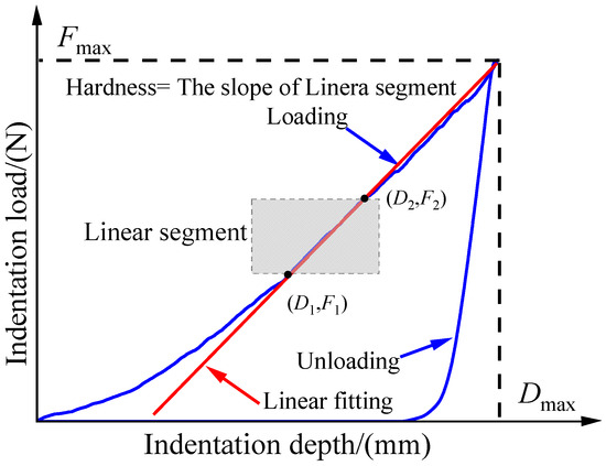
Figure 3.
Indentation loading–unloading curve.
2.2.2. Design of Experiment
After comparing and analyzing the research on using indentation loading method to measure grain hardness, it was found that loading speed, loading depth, needle tip taper, and moisture content have a significant impact on grain hardness measurements [17,20,31,32]. Based on the experimental environment, LS, LD, and DI were ultimately selected as the main factors affecting maize hardness, and the SLS of the loading curve obtained from the experiment was used as the response index of the experiment. Among them, the normal operating range of loading speed is between 0.10 and 2.00 mm/s. If it is too fast, it will lead to inaccuracies in the data collection of the instrument, and if the pressure head works at high speed for a long time, it will cause certain degree of damage. If it is too slow, it will prolong the running cycle of the experiment, reduce work efficiency, and increase the difficulty of data processing. A reasonable loading depth range can improve the accuracy of experimental data. Through preliminary experiments, it was found that if the loading depth is too deep, the maize grains will crack; moreover, if the loading depth is too small, it will cause the experiment to stop before the linear segment appears, resulting in unnecessary errors. Due to the difficulty in maintaining consistency in height among the selected maize grain samples, the concept of normalization was introduced, and the range of loading depth was set to 30–70% of the initial height of the polished sample. Pre-experiments were conducted, and it was found that maize grains did not undergo fragmentation. The essence of the indentation loading method is that the indenter does work on the test, and there is a reaction force inside the sample to resist deformation of the indenter. The more complex the shape of the indenter, the larger the hardness value obtained. Therefore, four types of indenters were selected for hardness measurement experiments. The distribution range of each sampled parameter is shown in Table 1. The most commonly used sampling methods for designing experiments include the full factorial, central composite, orthogonal array, Latin hypercube, and optimal Latin hypercube methods. The OPTLHD optimizes the order of the occurrence of each level in each column of the experimental design matrix, which can ensure a more uniform distribution of the factor levels at each sample point with excellent spatial filling and balance and avoid the appearance of gap areas [33,34]. Therefore, to ensure the uniformity of the sample points, the optimized Latin hypercube method with stratified sampling technique was used to sample the three input parameters, and the experiment collected a combination of 100 sample data. We applied the combination parameters of their respective variables to the maize hardness test, taking 100 maize hardness measurements.

Table 1.
Range of sampling parameters.
The above are the three variables and their respective ranges (types) for maize hardness test. The specific values of the three variable combinations in the test are summarized in Table A1 through the optimal Latin square design. We divided these 100 sets of data into the training and testing sets of the neural network with a 3:1 ratio. The training set contains 75 samples for training the network and the test set includes the remaining 25 samples to test the reliability of the model and evaluate its predictive performance.
2.3. MLM Prediction Model
MLMs are able to simulate highly nonlinear systems well and establish functional relationships between input and output variables. MLMs are essentially mathematical models that simulate biological neural networks for information processing. MLMs are based on the information transmission method of biological neural networks, abstracting, simplifying, and simulating the organizational structure and operational mechanism of the brain from the perspective of information processing. The essence of neural networks is to use numerical algorithms to connect a large number of neural nodes according to set rules and methods, forming a network model with high error tolerance, level of intelligence, independent learning ability, and parallel distribution. At present, MLMs have been widely applied in fields such as information technology, medicine, economics, engineering, transportation, and psychology [35]. This study took LD, LS, and DI as the input variables of the neural network system and SLS as the output variable to establish functional relationships. The topology of neural networks generally consists of input layers, hidden layers, and output layers. In this study, the number of neural nodes in the input layer is 3, representing three input variables. The output layer neuron node is maize hardness, and four neural network regression models were established, namely GA, SVM, LSTM, and RF models. The research technology roadmap is shown in Figure 4.
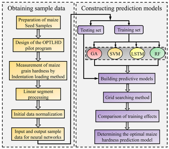
Figure 4.
The research process of machine learning models.
2.3.1. GA Prediction Model
The GA was proposed by Holland [36] as a approach to simulate the genetic mechanisms and biological evolution of natural selection. This algorithm possesses global search capability and can quickly search the solution space to obtain the global optimal solution for weights and thresholds. The GA network generates new subpopulations of individuals with high fitness values through operations such as crossover, mutation, and recombination and then undergoes multiple cycles to obtain the optimal individual [37]. Figure 5 shows the flowchart of the GA network structure. Based on backpropagation network (BP), GA used real number encoding to encode the initial weights and thresholds between each layer of neural nodes, transforming the solution space of the optimal problem into a search space that can be recognized by genetic algorithms. This study used mean square error as the fitness function and found the minimum fitness value after undergoing roulette chromosome selection, two-point crossover, and Gaussian mutation. We then assigned the weights and thresholds corresponding to the network to the initial neuron nodes and retrained the model again.
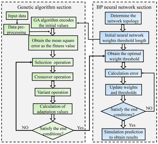
Figure 5.
GA optimization backpropagation network flowchart.
2.3.2. SVM Prediction Model
The SVM was proposed by Cortes and Vapnik [38] on the basis of statistical learning theory. The SVM model is commonly used to handle regression and classification problems. Based on the theory of structural risk minimization, the core of SVM is to divide data samples into both sides of a hyperplane, as shown in Figure 6a. The solid line represents the hyperplane, and the distance between two parallel dashed lines and the solid line is equal. In the SVM model, nonlinear mapping functions were used to map the training samples to the vicinity of the hyperplane to achieve the training process of the network. The SVM model has strong mathematical theoretical support, strong interpretability, and does not rely on statistical methods. Therefore, the problems of regression and classification have essentially been simplified. However, the initial samples and network parameters of the model have a significant impact on the network structure and prediction performance.
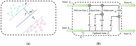
Figure 6.
(a) Schematic diagram of hyperplane structure; (b) LSTM internal structure diagram.
2.3.3. LSTM Prediction Model
The LSTM network was proposed by Hochreiter and Schmidhuber [39] and solved the problems of recurrent neural networks in long-term memory and gradient vanishing by adding gating systems. The optimized network can efficiently handle multivariable and multi-sample problems and exhibits extremely high memory performance. Compared with recurrent neural network, LSTM network has stronger data processing capabilities, especially in preserving historical data and making selective decisions. Therefore, LSTM is commonly used to solve time series analysis and regression analysis problems. Figure 6b shows the structure of the LSTM model, whose core is a cell unit with a memory function, which selectively updates the unit state in the form of a gate structure to achieve forgetting and memory functions. Each LSTM unit consists of three gate units, namely input gate, output gate, and forgetting gate. The forgetting gate limited the output value of the sigmoid function to 0~1 to control the amount of information flowing through the sigmoid layer. The closer the output value was to 1, the more historical information was retained, while the closer the output value was to 0, the more historical information was forgotten.
2.3.4. RF Prediction Model
The RF model was first proposed by Breiman [40]. As a type of machine-learning algorithm, RF is a powerful model based on bagging ensemble learning theory and is highly integrated with random subspaces. The RF model is composed of multiple decision trees, and the introduction of random variables on the basis of these decision trees provides advantages in terms of the model’s high accuracy, strong generalization ability, and fast convergence speed. It is widely used in solving classification and regression problems. In a regression analysis, RF prediction result is the average of all decision tree prediction results. In classification problems, the decision tree result with the highest number of voting results is the final prediction result.
2.4. Data Preprocessing
Through the maize hardness measurement experiment, 100 sets of experimental data and curves were obtained, but these data cannot be directly imported into the MLM as data input, because the MLM has dimensional requirements for the input of initial data. Dimensional differences between initial data can reduce the accuracy of the model and generate significant system errors, ultimately affecting the predictive performance of the entire network. Normalization is a commonly used data preprocessing method in MLMs, which can eliminate dimensional differences between data and reduce errors [41,42]. This study consistently restricts the input variables of the network to between 0 and 1; the formula for normalization is as follows:
where is the upper limit of the normalized interval; is the lower limit of the normalized interval; is the sample point of the data; is the minimum value of the data of any variable group; and is the maximum value of the data of any variable group.
3. Results and Discussion
3.1. Model Hyper-Parameter Optimization
In order to compare the predictive performance of the above four models for maize hardness, these models were assigned the optimized hyper-parameter, and the root mean square error (RMSE) and R-Square (R2) were used as analysis indicators for the four models. To visually compare the training effectiveness of the models, the prediction performance and fitting scatterplots of four regression model training and testing sets were analyzed. The error between the actual and predicted values of the model was also analyzed.
In this study, the grid search method [43] was used to optimize the number of hidden layer nodes in the four networks. Firstly, the approximate range of changes in the hidden layer nodes was determined using empirical formulas. Then, the trends of the changes in the R2 and mean absolute error (MAE) of the selected model under different hidden layer nodes were compared to find the optimal solution for the hyper-parameters of the network. The empirical formulas for the hidden layer, MAE, RMSE, and R2 are as follows:
where n is the number of neuron nodes in the hidden layer; m is the number of input variables; l is the number of neuron nodes in the output layer; and is any number between 0 and 10. In this study, is taken as 3, l is taken as 1, and N is the number of samples; and are the actual and predicted values, respectively; and is the mean value of .
3.1.1. Optimizing GA Network Parameter
The GA network added a fitness function on the basis of the backpropagation network, aiming to optimize the initial weights and thresholds between neurons in each layer, and the topology structure is consistent with the backpropagation network. The total length of the real number encoding was 41, the initial population size was set to 100, and the maximum evolutionary algebra was 30 generations. After repeated experiments and testing, it was found that the mutation probability has a minor impact on the network prediction performance, while the crossover probability (CP) has a significant impact. The mutation probability was set to 0.01, and the maximum number of iterations was 1000. The learning rate, minimum error of training objectives, display frequency, momentum factor, minimum performance gradient, and maximum allowable failure frequency were 0.01, 1 × 10⁻⁶, 0.01, 1 × 10⁻⁶, and 6 per 25 iterations, respectively. Moreover, the changes in the MAE and R2 of the GA network training and testing sets with the CP were analyzed, as shown in Figure 7. Obviously, the change in CP has a significant impact on both the MAE and R2. When the CP was 0.7, the R2 of the training and testing sets reached the maximum value, which happened to be the MAE value with the minimum error. Taking into account both the GA training set and the testing set, when the CP value is 0.7, the network is within the optimal operating parameters.
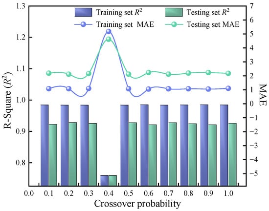
Figure 7.
Variation in MAE and R2 of GA networks with different crossover probabilities.
3.1.2. Optimizing SVM Network Parameters
The radial basis function was selected as the grain function of the SVM network, in which the penalty factor C and the radial basis parameter Gamma (g) had a significant impact on the prediction performance of the models. The changes in the training and testing sets’ MAE and R2 for the SVM model under different parameter combinations were analyzed, as shown in Figure 8a–d. Compared with the g parameter, the change in penalty factor C has a significant impact on the network MAE and R2. As the penalty factor C increases, the MAE first decreasesand then increases, while the R2 first increases to a specific value and then remains stable. When the penalty factor C is 1200, a turning point occurs, while when the g parameter increases to 0.7, the R2 in both the test and training sets reaches its peak. Combining the prediction performance of the training and testing sets of the network, the hyper-parameter penalty factors C and g of the SVM model were set to 1200 and 0.7, respectively.
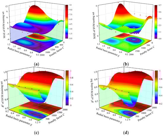
Figure 8.
Variation in MAE and R2 in the training set and testing set of SVM model with different parameter combinations. (a) Variation in MAE in training set of SVM model with different parameter combinations; (b) Variation in MAE in testing set of SVM model with different parameter combinations; (c) Variation in R2 in SVM model training set with different parameter combinations; (d) Variation in R2 in SVM model testing set with different parameter combinations.
3.1.3. Optimizing LSTM Network Parameters
As a deep learning algorithm, the LSTM adopts an Adam optimizer to significantly improve its learning speed and training effectiveness. We conducted experiments on and made comparisons of numerous hyper-parameters of the LSTM, among which the initial learning rate and the number of hidden layers have a significant impact on the prediction performance of the model. We analyzed the impact of the initial learning rate and the number of hidden layers on the MAE and R2 of the LSTM model training and testing sets under different parameter combinations, as shown in Figure 9a–d. Compared with the number of hidden layers, the initial learning rate has a greater impact on the model’s prediction performance. As the initial learning rate increases, the MAE first decreases and then increases, while the R2 first increases and then tends to stabilize. Unlike the trend of the changes in MAE, an increase in the number of hidden layers will first decrease and then increase the MAE value of the model. On the contrary, R2 indicates that increasing the number of hidden layers appropriately can improve the predictive performance of the model. However, when the number of hidden layers reaches a certain value, the model will exhibit obvious overfitting, which will decrease the predictive performance of the model. By comprehensively analyzing the predictive performance of the model, the number of hidden layers and an initial learning rate of 60 and 0.08 were optimal for the LSTM model, respectively.
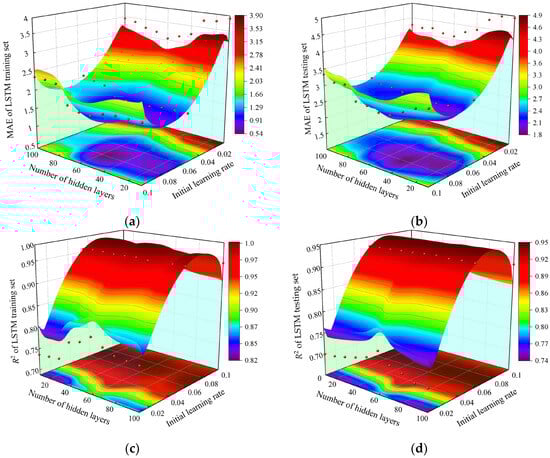
Figure 9.
Variation in MAE and R2 in the training set and testing set of LSTM model with different parameter combinations. (a) Variation in MAE in training set of LSTM model with different parameter combinations; (b) Variation in MAE in testing set of LSTM model with different parameter combinations; (c) Variation in R2 in LSTM model training set with different parameter combinations; (d) Variation in R2 in LSTM model testing set with different parameter combinations.
3.1.4. Optimizing RF Network Parameters
The number of decision trees and the maximum number of leaves are the two parameters that have the greatest impact on the RF model. The variation trends of MAE and R2 in the training and testing sets of the RF model under different parameter combinations were analyzed, as shown in Figure 10a–d. Compared with the number of decision trees, the change in the maximum number of leaves will cause significant fluctuations in the MAE of the model, first decreasing and then increasing. The turning point will appear when the maximum number of leaves is 3; at this point, the prediction performance of the network is optimal. The increase in the number of decision trees has little impact on the changes in MAE; even increasing the number of decision trees will not improve the training effect of the model and instead will make the network more complex. However, increasing the number of decision trees will cause R2 to first increase and then decrease, indicating that as the number of decision trees increases, the model will experience initial overfitting and gradually move towards a stable state. Taking into account the predictive performance of the model, the number of decision trees and the maximum number of leaves for the RF model were set to 50 and 3, respectively.
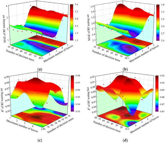
Figure 10.
Variation in MAE and R2 in the training set and testing set of RF model with different parameter combinations. (a) Variation in MAE in training set of RF model with different parameter combinations; (b) Variation in MAE in testing set of RF model with different parameter combinations; (c) Variation in R2 in RF model training set with different parameter combinations; (d) Variation in R2 in RF model testing set with different parameter combinations.
3.2. Analysis of Training Set Prediction Effect
The neural network model first trains the data provided by the training set, and the prediction performance of the training set reflects the prediction trend of the entire network. Therefore, the change trend between the true and predicted values of the four model training sets was analyzed first, as shown in Figure 11a–d. It can be observed that there is only a small portion of sample points with significant errors between the predicted values of the training set and the true values, while the errors between all other samples are within a reasonable range of variation. From the overall prediction trend, the actual change trend of the sample points is highly consistent with the predicted trend of the model. From the magnitude of data changes, it can be seen that the training set data fitting performance of the GA and SVM models is more reliable than that of the other two models. Although the LSTM and RF models still have certain advantages when it comes to predicting trends, they demonstrate significant disadvantages in terms of model accuracy. The prediction performances of the training sets are ranked in descending order as follows: SVM, GA, LSTM, and RF.
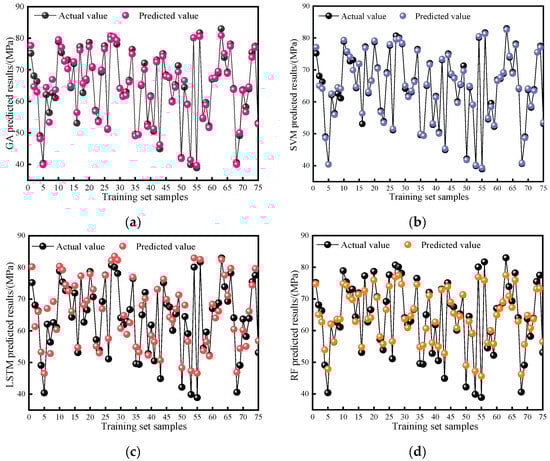
Figure 11.
Comparison of model training set prediction effect. (a) GA training set prediction effect (b) SVM training set prediction effect; (c) LSTM training set prediction effect; (d) RF training set prediction effect.
Scatterplots can effectively represent the overall dispersion of sample data, facilitating the evaluation of the predictive performance of the model. Based on this, scatterplots were drawn for the true sample points of the training and testing sets and the predicted values of the four models, and their respective fitting lines are as shown in Figure 12a–d. It is not difficult to see from the fitting scatterplot that there is a good linear relationship between the 75 samples used in the training set for training the network and the predicted values of each model, and the sample points are relatively evenly distributed on both sides of the fitting line, with fewer significant deviation points. This indicates that the sample points in the model training set have a high degree of agreement with the predicted values of the model, and the model training is effective. The degrees of dispersion of the sample points in the models are listed in descending order as follows: SVM, GA, RF, and LSTM.
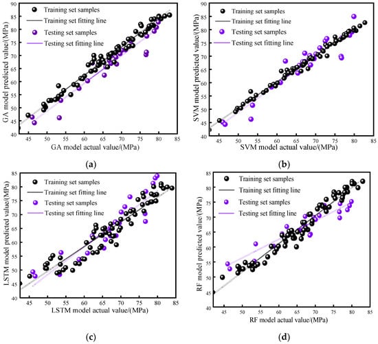
Figure 12.
Comparison of model training set and testing set fitted scatterplot. (a) GA-fitted scatterplot; (b) SVM-fitted scatterplot; (c) LSTM-fitted scatterplot; (d) RF-fitted scatterplot.
The amplitude of the error plot can to some extent reflect the fluctuation of a set of data, and the model can be evaluated to different degrees based on the size of the data sample points. To further compare the predictive performance of the selected model training set, the error between the true values of the samples and the predicted values of the model was analyzed, as shown in Figure 13. From the error chart, it can be seen that the error between the 75 samples in the training set and the predicted values of the model is relatively flat, with an error range of −8 to 8. The amplitude of error changes in the model training set can be arranged in ascending order as follows: SVM, GA, LSTM, and RF. This order is similar to the results obtained from analyzing the scatterplots. Finally, comparing the evaluation indicators of the model is more intuitive and persuasive. We calculated the R2 and RMSE of the model training and testing sets, as shown in Table 2. It can be seen that the R2 of the four selected model training sets is above 0.91, and the RMSE is less than 3.6, indicating that the overall training effect of the training set is good. Among them, the R2 of the LSTM model is the smallest, 0.91435, while the RMSE is the largest, 3.5413. Compared with the other three models, the R2 values of the SVM, GA, and RF are 8.56%, 7.62%, and 6.44% higher than the LSTM, respectively, while the RMSE values of the SVM, GA, and RF are 72.58%, 60%, and 5.3% lower than the LSTM, respectively. The maximum errors between the true and predicted values of the training set in the four models are 3.2708 (SVM), 4.3151 (GA), 7.9228 (RF), and 7.6466 (LSTM), and the minimum errors are 0.0384 (SVM), 0.0195 (GA), 0.0687 (RF), and 0.0048 (LSTM), respectively. Based on the above analysis, the predictive abilities of the training set are as follows: SVM, GA, RF, and LSTM, in descending order.
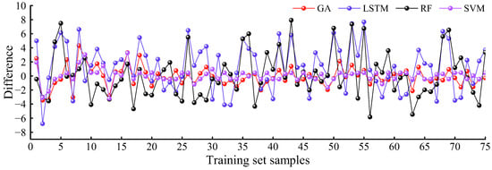
Figure 13.
Error fluctuations between the actual and predicted values of the training set.
Table 2.
Root mean square error (RMSE) and R-Square (R2) for different models.
3.3. Analysis of Testing Set Prediction Effect
The testing set of neural networks is used to test the trained network model. Generally, the predictive performance of the test set determines the data fitting and generalization ability of the entire network model to a certain extent. Except for the 75 samples used in the training set, the remaining 25 sets of data will be used as sample points in the test set to evaluate the predictive performance of the model. Similar to the analysis method of the training set, Figure 14a–d shows the trend of changes between the 25 samples in the test set and the predicted values of the four models. From the figure, it can be seen that, compared with the training set, the similarity between the predicted values and the actual values is significantly reduced, which is related to the prediction accuracy of the model itself. However, the trend of the predicted values is basically consistent with the actual values, with a relatively large error between the two, indicating that the model does not have overfitting. According to the trend of data changes, the data-fitting performance of the GA and SVM model test sets is significantly better than that of the other two models, which is consistent with the results of the training set. We ranked the models in ascending order according to the similarity of their predicted trends as follows: RF, LSTM, SVM, and GA.
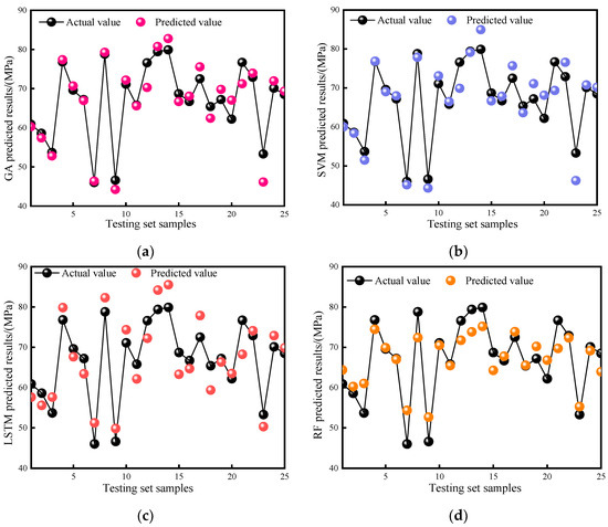
Figure 14.
Comparison of model testing set prediction effect. (a) GA testing set prediction effect; (b) SVM testing set prediction effect; (c) LSTM testing set prediction effect; (d) RF testing set prediction effect.
Observing the scatterplot of fitting the 25 sample points in the test set, it can be seen that, like in the training set, there is also a linear correlation between the 25 samples used to test the predictive performance of the model, but the fitting effect is significantly inferior to that of the training set. Overall, the test set sample points are evenly distributed on both sides of the fitting line, but there are individual data points that deviate from the fitting line. We ranked them in terms of the degree of dispersion of the test set data as follows: GA, SVM, RF, and LSTM, in descending order. In addition, the errors in the test set were also statistically analyzed, as shown in Figure 15. It can be seen from the figure that the number of errors between the actual and predicted values in the test set has increased. Among the four models, the GA has the smallest error, followed by the SVM and LSTM, and the RF has the largest error. During network operation, it was found that the running speed of the LSTM and GA networks is longer than that of the RF and SVM, because the difference in computational principles between the models is significant.
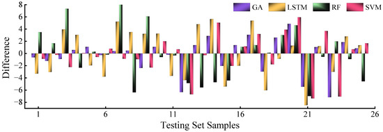
Figure 15.
Error fluctuations between the actual and predicted values of the testing set.
Finally, the two evaluation metrics, R2 and RMSE, of the test set were compared, as shown in Table 2. The R2 of all four models in the test set is above 0.84, and the range of RMSE variation is between 2.8 and 4.2. Among them, the R2 of the LSTM is the smallest, 0.84443, and the RMSE of the RF is 4.0137. The R2 of the GA, SVM, and RF increased by 9.85%, 6.83%, and 5.06%, respectively, on the basis of the LSTM. The RMSE of the GA, SVM, and LSTM decreased by 31.14%, 19.22%, and 2.82%, respectively, on the basis of the RF. The maximum errors between the actual and predicted values of the model are 7.1609 (GA), 7.3419 (SVM), 0.88714 (RF), and 0.84443 (LSTM), respectively. The minimum errors are 0.204 (GA), 0.06482SVM), 0.1359 (RF), and 0.867 (LSTM), respectively.
By comprehensively comparing the overall predictive performance of the four network model testing sets, it was found that the GA model outperforms the other models in terms of both the fitting of the scatterplot between the actual and predicted values and the error fluctuation in the testing set. The sorting results of the testing set based on the predicted performance are the GA, SVM, LSTM, and RF. Combining the training and testing sets, the overall prediction performance of the GA model is optimal, with a small range of error fluctuations. It also indicates that the GA model can improve the training speed and prediction performance of the backpropagation model [44]. During the training process, the SVM model actually experienced overfitting, and the optimization method for the hyper-parameters of the network still needs improvement. The most important feature of the RF model is the randomness of the training, which has no restrictions on the input and output of variables. In terms of the importance of variables, the results were as follows: DI, LD, and LS. This outcome is consistent with the research results in the literature [31]. However, the RF model is not highly sensitive to experimental data on maize grain hardness. The LSTM model is a deep learning network with many variables that affect network accuracy, and the training time of the general network is relatively long. Therefore, by comprehensively analyzing the prediction accuracy and efficiency of various models, the GA model is more suitable for predicting maize grain hardness.
In order to more intuitively and accurately demonstrate the predictive ability of the model on initial data, the predicted values of each of the four models, along with the maize hardness values measured in the indentation loading test, are summarized together. The first 75 sets of data are the training set samples of the model, and the remaining 25 sets of data are the testing set samples. The specific values of LS, LD, and DI designed through the optimal Latin square method are listed in Table A1.
3.4. Microstructure Analysis of Maize Surface before and after Compression
We used the direct sample preparation method to grind five randomly selected maize grains into a square sample with a height of 2 mm. Four samples were subjected to loading tests using four DI values, while the other sample was untreated. Then, the sample was adhered to the conductive adhesive platform of the electron microscope and subjected to a gold-spraying treatment using an ion-sputtering instrument. The internal structure of the maize was observed via a scanning electron microscope. The scanning electron microscope is a tungsten wire scanning electron microscope (SEM, Hitachi-S3400N) with a resolution of 3.0 nm (30 kV) and a BSE resolution of 4.0 nm (30 kV). The magnitude of enlargement is 5~300,000 times, as shown in Figure 16a. The outer layer of maize endosperm is composed of many cells, which are wrapped in starch granules and closely connected to the protein matrix.
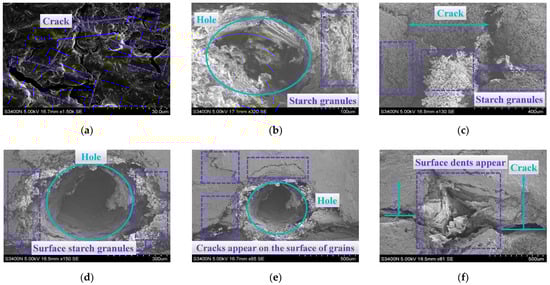
Figure 16.
Endosperm microstructure of maize grains before and after loading with different types of indenters. (a) Untreated seeds, magnified 1500 times; (b) A 30° conical indenter, magnified 320 times; (c) A 30° triangular indenter, magnified 130 times; (d) A 30° spherical steel needle indenter, magnified 150 times; (e) A 30° spherical steel needle indenter, magnified 85 times; and (f) A 30° quadrangular indenter, magnified 81 times. Note: Figure (d,e) are the same image. In order to showcase the changes in surface structure, the magnification of the two images is different.
There are many small pores inside the starch particles, which are spherical in shape and have an unsmooth surface. This may be due to the breakage of protein matrix filaments during the natural drying process of maize, resulting in the formation of fine pore texture shapes in the endosperm [45]. From Figure 16b, it can be seen that the arrangement of starch particles inside the maize endosperm is relatively tight. Compression can disrupt the cohesion between starch particles, causing the crushed starch particles to be pushed around the indentation and form cracks. As shown in Figure 16c–f, after compression, obvious cracks and gaps will form around the indentation of the maize endosperm. The deformation of these cracks is influenced by the shape and hardness of the indenter used, with the pyramid-shaped indenter having the greatest degree of destruction to the surface of the maize. During the pressing process, the indenters compress the wall and bottom structures, and the internal structure of the grain resists this deformation, eventually forming cracks or breaking after exceeding the maximum binding force. Hardness is the ability of a material to resist deformation and damage within a small volume on its surface, and the shape of the indenter has a significant impact on the degree of structural damage inside the grains. This also deepens our understanding of the hardness characteristics of maize grains at the micro level. This conclusion was consistent with the importance degree results of the factors affecting maize hardness in the RF model.
4. Conclusions
(1) The hardness of the endosperm part of the selected maize grains was determined by using the indentation loading curve method and a texture analyzer. It was shown that under different types of loading indenters, the hardness of the maize endosperm ranges from 38 to 81 MPa when the loading speed varies from 0.2 to 1.6 mm/s and the loading depth varies from 30 to 70% of the sample height. The prediction ranges of maize hardness for the four network models are as follows: the GA model predicts the range from 39.71 to 82.77 MPa, the SVM model predicts the range from 39.35 to 84.95 MPa, the RF model predicts the range from 45.65 to 77.53 MPa, and the LSTM model predicts the range from 44.28 to 83.94 MPa.
(2) The RF model ranks DI, LD, and LS in order of importance in terms of the input variables. After analyzing the internal structure of the maize grains from a microscopic perspective, it was found that the surface of the maize endosperm contains a large number of starch particles, which are arranged tightly. The degree of damage to the surface of the grains varies with the different shapes of the indenters. The more complex the shape of the indenter, the more severe the structural damage to the internal grains, and obvious cracks will appear on the surface of the grains. When the loading pressure reaches a certain value, the grains will be crushed.
(3) After optimizing the hyper-parameters of the model using the grid search method, we compared the RMSE and R2 of the training and testing sets of the GA, SVM, LSTM, and RF regression models. The results showed that the GA model had the best prediction performance, with the smallest error between the actual and predicted values. The RMSE values of the training and testing sets are 1.4308 and 2.8441, respectively, and the R2 values are 0.98402 and 0.92761, respectively. This indicated that a genetic algorithm (GA) can significantly optimize the weights and thresholds of the initial network, thereby improving the prediction performance of the network. Compared to other models, the SVM model exhibited overfitting, while the RF and LSTM models exhibited significant errors between actual and predicted values, resulting in a poor overall prediction performance. Therefore, the GA model can serve as a stable and reliable regression model to provide maize hardness information for industries such as transportation, processing, and milling.
(4) This study focuses on seed maize with a moisture content of 36.54%. The grain hardness was measured using the indentation loading method, and the measured hardness information was imported into mechanical learning models to predict the maize hardness information. This can be used for cultivating high-quality varieties and industrial classification processing, improving grain quality, minimizing raw material loss, and improving processing efficiency. However, this study only investigated maize grains with the same moisture content for a single variety, without involving changes in maize hardness information between different moisture contents or the sensitivity of network models to such data. In addition, there is still room for improvement in the selection of network models for predicting hardness information, with only four common regression models selected here. In future research, we will increase the variation in hardness between different varieties under different moisture contents, as well as the response of each variety to the model. In addition, we will continue to study deep learning and its optimization algorithms to provide reliable models for predicting the hardness information of agricultural materials.
Author Contributions
Conceptualization, F.D. and X.S.; methodology, X.S.; software, H.L.; writing—original draft preparation, H.L.; writing—review and editing, H.L.; experiment, H.C. and Q.X.; supervision, F.Z. and X.S. All authors have read and agreed to the published version of the manuscript.
Funding
This research was funded by Youth Fund of the National Natural Science Foundation of China (Grant No.32101636).
Data Availability Statement
Data will be made available on request.
Acknowledgments
The authors would like to thank the reviewers for their hard work. The authors also acknowledge the financial support for this work provided by the Youth Fund of the National Natural Science Foundation of China (Grant No.32101636).
Conflicts of Interest
The authors declare that they have no known competing financial interests or personal relationships that could have appeared to influence the work reported in this paper.
Appendix A
Table A1.
Maize grain hardness measurements and model predictions.
Table A1.
Maize grain hardness measurements and model predictions.
| Number | LS (mm/s) | LD(%) | DI | Hardness (MPa) | GA | SVM | LSTM | RF |
|---|---|---|---|---|---|---|---|---|
| 1 | 0.858 | 61.5 | 3 | 75.2 | 77.6793 | 77.1186 | 80.1878 | 74.7386 |
| 2 | 0.752 | 53.0 | 2 | 68.1 | 64.6445 | 65.0205 | 61.3048 | 65.0596 |
| 3 | 0.494 | 32.4 | 3 | 66.3 | 62.9560 | 64.1105 | 66.0335 | 62.7279 |
| 4 | 0.433 | 55.1 | 1 | 49.1 | 48.1072 | 48.6574 | 53.2738 | 53.9378 |
| 5 | 1.494 | 34.0 | 1 | 40.4 | 39.8996 | 40.3616 | 46.5257 | 47.8861 |
| 6 | 1.176 | 36.9 | 3 | 62.1 | 64.4225 | 62.5252 | 67.0208 | 62.0313 |
| 7 | 0.358 | 31.6 | 2 | 56.4 | 53.3637 | 55.9586 | 52.8238 | 56.4974 |
| 8 | 0.888 | 40.1 | 3 | 62.6 | 66.9152 | 64.5260 | 69.2150 | 63.5969 |
| 9 | 0.903 | 51.0 | 2 | 61.1 | 63.6378 | 64.1234 | 60.3918 | 63.6307 |
| 10 | 1.433 | 63.1 | 4 | 78.9 | 79.5367 | 79.3572 | 80.3839 | 74.8125 |
| 11 | 1.524 | 62.3 | 3 | 75.4 | 77.1389 | 75.8569 | 79.1988 | 74.2628 |
| 12 | 1.342 | 52.2 | 3 | 72.7 | 72.7195 | 74.1361 | 74.5175 | 70.7549 |
| 13 | 0.13 | 43.7 | 3 | 73.1 | 70.2840 | 69.8846 | 72.5521 | 69.7725 |
| 14 | 1.403 | 33.6 | 4 | 64.3 | 64.9010 | 64.7512 | 66.1458 | 62.8923 |
| 15 | 1.585 | 52.6 | 3 | 71.9 | 72.5455 | 71.9805 | 74.2258 | 71.4070 |
| 16 | 0.221 | 36.5 | 2 | 53.1 | 56.4130 | 56.3708 | 54.7594 | 54.8164 |
| 17 | 0.267 | 51.4 | 4 | 77.3 | 76.1667 | 76.8558 | 77.2953 | 72.6166 |
| 18 | 0.797 | 37.7 | 3 | 62.7 | 65.6436 | 63.1587 | 68.1496 | 63.6333 |
| 19 | 0.524 | 39.3 | 3 | 66.6 | 67.1053 | 66.5256 | 69.4927 | 64.0426 |
| 20 | 1.024 | 56.3 | 4 | 78.7 | 77.2508 | 79.1565 | 77.9446 | 75.9578 |
| 21 | 0.721 | 47.0 | 3 | 70.7 | 71.0211 | 70.3974 | 73.0788 | 70.4179 |
| 22 | 1.07 | 38.5 | 2 | 57.2 | 56.8418 | 56.7503 | 55.1722 | 58.0825 |
| 23 | 0.979 | 32.8 | 2 | 53.9 | 53.4626 | 53.4043 | 53.0031 | 55.8158 |
| 24 | 0.297 | 66.4 | 2 | 69.2 | 69.9637 | 68.7452 | 66.9145 | 66.6189 |
| 25 | 0.615 | 53.4 | 4 | 77.6 | 76.5786 | 78.0240 | 77.4980 | 74.0144 |
| 26 | 0.342 | 67.2 | 1 | 51.1 | 51.3815 | 51.5426 | 57.5752 | 56.6073 |
| 27 | 1.418 | 68.0 | 3 | 80.7 | 79.5844 | 79.5037 | 82.1673 | 76.9007 |
| 28 | 0.933 | 68.8 | 3 | 80.1 | 80.4667 | 79.6607 | 83.5416 | 77.4458 |
| 29 | 0.57 | 64.8 | 3 | 78.1 | 79.3534 | 78.3741 | 82.3058 | 74.6589 |
| 30 | 0.403 | 51.4 | 2 | 64.1 | 64.0369 | 65.0644 | 60.7573 | 63.6654 |
| 31 | 0.706 | 30.8 | 3 | 61.9 | 61.4761 | 61.4982 | 64.8418 | 60.8856 |
| 32 | 1.221 | 47.8 | 2 | 63.0 | 61.8522 | 63.4548 | 58.8934 | 64.6603 |
| 33 | 1.6 | 57.1 | 2 | 66.7 | 66.1024 | 66.2383 | 62.5600 | 66.9238 |
| 34 | 1.267 | 56.7 | 3 | 76.5 | 74.9749 | 76.0433 | 76.9230 | 74.5833 |
| 35 | 0.145 | 59.9 | 1 | 49.6 | 49.0214 | 50.0251 | 54.8966 | 54.8586 |
| 36 | 1.327 | 54.7 | 1 | 49.4 | 49.4890 | 49.3452 | 53.2754 | 55.3952 |
| 37 | 0.206 | 35.3 | 3 | 65.0 | 65.2875 | 65.4468 | 68.0024 | 60.6685 |
| 38 | 1.509 | 42.9 | 4 | 72.1 | 70.0776 | 71.6524 | 70.2352 | 71.1017 |
| 39 | 1.312 | 31.2 | 2 | 52.8 | 52.0068 | 53.2271 | 52.2897 | 56.1437 |
| 40 | 0.161 | 45.8 | 2 | 61.8 | 61.4489 | 61.3578 | 58.5165 | 62.7182 |
| 41 | 0.676 | 63.9 | 1 | 50.5 | 51.3200 | 50.0401 | 56.5092 | 54.9905 |
| 42 | 0.585 | 44.6 | 4 | 73.1 | 72.4358 | 73.4093 | 73.1101 | 72.8603 |
| 43 | 1.13 | 47.4 | 1 | 44.9 | 46.2653 | 45.3288 | 50.7008 | 52.8229 |
| 44 | 0.979 | 54.2 | 3 | 75.1 | 74.2551 | 74.5589 | 76.2859 | 73.8603 |
| 45 | 1.373 | 43.3 | 3 | 68.4 | 67.9096 | 68.8421 | 69.9208 | 68.9786 |
| 46 | 0.842 | 60.3 | 2 | 67.5 | 67.7208 | 67.3406 | 64.2838 | 65.4786 |
| 47 | 1.388 | 30.4 | 3 | 60.1 | 59.7684 | 59.6517 | 63.4095 | 60.8247 |
| 48 | 1.555 | 38.1 | 3 | 65.3 | 64.4396 | 65.5619 | 66.9068 | 64.5259 |
| 49 | 1.206 | 45.4 | 3 | 71.3 | 69.3358 | 69.6647 | 71.2842 | 71.3713 |
| 50 | 0.115 | 40.5 | 1 | 42.2 | 41.8396 | 41.7715 | 48.3311 | 48.9927 |
| 51 | 0.373 | 33.2 | 4 | 64.5 | 66.5993 | 64.9368 | 68.1035 | 62.9332 |
| 52 | 0.448 | 41.3 | 2 | 59.1 | 58.9656 | 59.1496 | 56.6068 | 59.2060 |
| 53 | 1.145 | 37.3 | 1 | 39.9 | 41.4313 | 40.1941 | 47.3411 | 47.2515 |
| 54 | 1.297 | 69.2 | 3 | 80.1 | 80.1920 | 80.5304 | 82.9970 | 76.9057 |
| 55 | 0.661 | 34.9 | 1 | 38.9 | 39.7142 | 39.3545 | 46.5766 | 45.6451 |
| 56 | 0.479 | 62.7 | 4 | 81.7 | 80.5237 | 81.2670 | 82.5232 | 75.8693 |
| 57 | 0.691 | 34.4 | 2 | 54.5 | 54.7792 | 54.9422 | 53.7506 | 56.1823 |
| 58 | 0.873 | 41.7 | 2 | 59.6 | 58.8711 | 58.4296 | 56.5770 | 60.0761 |
| 59 | 0.948 | 30.0 | 2 | 52.2 | 51.6550 | 52.6587 | 52.0128 | 55.8043 |
| 60 | 0.782 | 35.7 | 4 | 67.0 | 67.2742 | 66.5643 | 68.3812 | 64.9563 |
| 61 | 0.494 | 59.5 | 2 | 67.2 | 67.4514 | 67.6516 | 64.0505 | 66.9347 |
| 62 | 1.115 | 65.2 | 2 | 68.8 | 69.5508 | 69.2411 | 66.1807 | 69.0721 |
| 63 | 1.085 | 65.6 | 4 | 83.0 | 80.8695 | 82.5530 | 82.4631 | 77.5252 |
| 64 | 0.1 | 53.4 | 3 | 73.9 | 75.1569 | 74.3463 | 77.5722 | 70.9103 |
| 65 | 0.464 | 42.1 | 3 | 69.3 | 68.8275 | 68.8354 | 71.0705 | 67.3143 |
| 66 | 1.191 | 61.9 | 3 | 78.2 | 77.4106 | 77.7561 | 79.6973 | 75.9553 |
| 67 | 0.191 | 50.6 | 2 | 64.1 | 63.7439 | 64.3127 | 60.4834 | 62.8886 |
| 68 | 0.327 | 36.1 | 1 | 40.6 | 39.9866 | 40.8748 | 46.9411 | 46.2117 |
| 69 | 0.964 | 57.9 | 1 | 49.1 | 50.0417 | 48.6529 | 54.4057 | 55.6349 |
| 70 | 0.539 | 50.2 | 2 | 63.7 | 63.4227 | 64.1386 | 60.2238 | 64.8700 |
| 71 | 1.539 | 38.9 | 2 | 58.2 | 56.6142 | 58.6589 | 55.0959 | 60.7751 |
| 72 | 1.055 | 32.0 | 4 | 63.9 | 64.5729 | 63.4505 | 66.1352 | 63.6514 |
| 73 | 0.903 | 48.6 | 4 | 75.5 | 73.9372 | 75.5386 | 74.3870 | 73.1514 |
| 74 | 0.312 | 58.3 | 3 | 77.5 | 77.0240 | 77.0397 | 79.6208 | 73.3080 |
| 75 | 1.358 | 64.3 | 1 | 53.1 | 52.8085 | 53.5515 | 56.8090 | 56.4638 |
| 76 | 0.767 | 44.1 | 2 | 60.9 | 60.2632 | 60.0277 | 57.6156 | 64.3905 |
| 77 | 1.236 | 39.7 | 2 | 58.6 | 57.4005 | 58.3864 | 55.5796 | 60.2598 |
| 78 | 1.009 | 66.8 | 1 | 53.7 | 52.7969 | 51.4872 | 57.6350 | 61.0312 |
| 79 | 0.827 | 60.7 | 3 | 76.8 | 77.3779 | 76.8648 | 79.8499 | 74.4751 |
| 80 | 0.63 | 68.4 | 2 | 69.6 | 70.6859 | 69.0368 | 67.6464 | 69.9052 |
| 81 | 1.252 | 58.7 | 2 | 67.2 | 66.9506 | 67.9803 | 63.4219 | 67.0204 |
| 82 | 0.736 | 49.0 | 1 | 46.0 | 46.3880 | 45.1469 | 51.2320 | 54.3548 |
| 83 | 0.252 | 63.5 | 3 | 78.8 | 79.2664 | 77.8685 | 82.3111 | 72.4188 |
| 84 | 0.418 | 45.0 | 1 | 46.6 | 44.2351 | 44.3052 | 49.8285 | 52.6769 |
| 85 | 0.388 | 48.2 | 3 | 71.1 | 72.1821 | 73.1042 | 74.3600 | 70.5142 |
| 86 | 1.1 | 55.5 | 2 | 65.8 | 65.5960 | 66.4977 | 62.1466 | 65.4816 |
| 87 | 1.039 | 46.6 | 3 | 76.6 | 70.2823 | 69.9029 | 72.2421 | 71.7513 |
| 88 | 0.282 | 67.6 | 3 | 79.4 | 80.7679 | 79.1365 | 84.1882 | 73.8329 |
| 89 | 0.645 | 69.6 | 4 | 79.9 | 82.7700 | 84.9483 | 85.5306 | 75.1910 |
| 90 | 0.176 | 57.5 | 2 | 68.7 | 66.6824 | 66.6787 | 63.3013 | 64.2805 |
| 91 | 0.555 | 61.1 | 2 | 66.7 | 68.0765 | 67.8645 | 64.6989 | 67.7930 |
| 92 | 0.6 | 55.9 | 3 | 72.5 | 75.5567 | 75.6966 | 77.8771 | 73.8728 |
| 93 | 1.57 | 49.4 | 2 | 65.4 | 62.4348 | 63.6315 | 59.3768 | 65.5359 |
| 94 | 1.464 | 66.0 | 2 | 67.2 | 69.8064 | 71.1005 | 66.3330 | 70.2209 |
| 95 | 1.448 | 59.1 | 2 | 62.2 | 67.0518 | 68.1354 | 63.4856 | 66.8242 |
| 96 | 0.812 | 70.0 | 2 | 76.7 | 71.2430 | 69.3581 | 68.2486 | 69.7254 |
| 97 | 1.282 | 49.8 | 4 | 72.9 | 73.9487 | 76.5850 | 74.1011 | 72.3672 |
| 98 | 1.479 | 46.2 | 1 | 53.3 | 46.1391 | 46.2393 | 50.3027 | 55.2773 |
| 99 | 0.236 | 42.5 | 4 | 70.1 | 71.9640 | 70.7809 | 72.8929 | 69.1834 |
| 100 | 1.161 | 40.5 | 4 | 68.5 | 69.3507 | 70.1782 | 69.8549 | 63.9372 |
Note: In the fourth column of the table, 1 represents a 30° conical indenter, 2 represents a spherical indenter, 3 represents a 30° triangular indenter, and 4 represents a 30° quadrangular indenter.
References
- Khan, S.N.; Li, D.P.; Maimaitijiang, M. A Geographically Weighted Random Forest Approach to Predict Corn Yield in the US Corn Belt. Remote Sens. 2022, 14, 2843. [Google Scholar] [CrossRef]
- Hernandez, G.L.; Aguilar, C.H.; Pacheco, A.D.; Sibaja, A.M.; Orea, A.A.C.; de Jesus Agustin Flores Cuautle, J. Thermal properties of maize seed components. Cogent Food Agric. 2023, 9, 2231681. [Google Scholar] [CrossRef]
- Singh, S.; Bekal, S.; Duan, J.; Singh, V. Characterization and Comparison of Wet Milling Fractions of Export Commodity Corn Originating from Different International Geographical Locations. Starch-Starke 2023, 75, 2200280. [Google Scholar] [CrossRef]
- Borrás, L.; Caballero-Rothar, N.N.; Saenz, E.; Segui, M.; Gerde, J.A. Challenges and opportunities of hard endosperm food grade maize sourced from South America to Europe. Eur. J. Agron. 2022, 140, 126596. [Google Scholar] [CrossRef]
- Tamagno, S.; Greco, I.A.; Almeida, H.; Di Paola, J.C.; Martí Ribes, F.; Borrás, L. Crop Management Options for Maximizing Maize Kernel Hardness. Agron. J. 2016, 108, 1561–1570. [Google Scholar] [CrossRef]
- Bhatia, G.; Juneja, A.; Bekal, S.; Singh, V. Wet milling characteristics of export commodity corn originating from different international geographical locations. Cereal Chem. 2021, 98, 794–801. [Google Scholar] [CrossRef]
- HernanA, C.-N.; EdgarO, O.-R.; Ortiz, A.; Matta, Y.; Hoyos, J.S.; Buitrago, G.D.; Martinez, J.D.; Yanquen, J.J.; Chico, M.; Martin, V.E.S.; et al. Effects of corn kernel hardness and grain drying temperature on particle size and pellet durability when grinding using a roller mill or hammermill. Anim. Feed. Sci. Technol. 2021, 271, 114715. [Google Scholar] [CrossRef]
- Wang, J.; Yang, C.; Zhao, W.; Wang, Y.; Qiao, L.; Wu, B.; Zhao, J.; Zheng, X.; Wang, J.; Zheng, J. Genome-wide association study of grain hardness and novel Puroindoline alleles in common wheat. Mol. Breeding 2022, 42, 40. [Google Scholar] [CrossRef]
- Gustin, J.L.; Jackson, S.; Williams, C.; Patel, A.; Armstrong, P.; Peter, G.F.; Settles, A.M. Analysis of Maize (Zea mays) Kernel Density and Volume Using Microcomputed Tomography and Single-Kernel Near-Infrared Spectroscopy. J. Agric. Food Chem. 2013, 61, 10872–10880. [Google Scholar] [CrossRef]
- Martínez, R.D.; Cirilo, A.G.; Cerrudo, A.; Andrade, F.H.; Izquierdo, N.G. Environment affects starch composition and kernel hardness in temperate maize. J. Sci. Food Agric. 2022, 102, 5488–5494. [Google Scholar] [CrossRef]
- Fox, G.P.; Osborne, B.; Bowman, J.; Kelly, A.; Cakir, M.; Poulsen, D.; Inkerman, A.; Henry, R. Measurement of genetic and environmental variation in barley (Hordeum vulgare) grain hardness. J. Cereal Sci. 2007, 46, 82–92. [Google Scholar] [CrossRef]
- Qiao, M.; Xu, Y.; Xia, G.; Su, Y.; Lu, B.; Gao, X.; Fan, H. Determination of hardness for maize kernels based on hyperspectral imaging. Food Chem. 2022, 366, 130559. [Google Scholar] [CrossRef] [PubMed]
- Du, Z.; Hu, Y.; Ali Buttar, N.; Mahmood, A. X-ray computed tomography for quality inspection of agricultural products: A review. Food Sci. Nutr. 2019, 7, 3146–3160. [Google Scholar] [CrossRef] [PubMed]
- Pierna, J.A.F.; Baeten, V.; Williams, P.J.; Sendin, K.; Manley, M. Near Infrared Hyperspectral Imaging for White Maize Classification According to Grading Regulations. Food Anal. Methods 2019, 12, 1612–1624. [Google Scholar] [CrossRef]
- Caporaso, N.; Whitworth, M.B.; Fisk, I.D. Near-Infrared spectroscopy and hyperspectral imaging for non-destructive quality assessment of cereal grains. Appl. Spectrosc. Rev. 2018, 53, 667–687. [Google Scholar] [CrossRef]
- Jose I Varela, N.D.M.; Infante, V.; Kaeppler, S.M.; de Leon, N.; Spalding, E.P. A novel high-throughput hyperspectral scanner and analytical methods for predicting maize kernel composition and physical traits. Food Chem. 2022, 391, 133264. [Google Scholar] [CrossRef]
- Song, X.; Dai, F.; Zhang, X.; Sun, Y.; Zhang, F.; Zhang, F. Experimental analysis of the hardness measurement method of pea indentation loading curve based on response surface. J. China Agric. Univ. 2020, 25, 158–165. [Google Scholar] [CrossRef]
- Maryami, Z.; Azimi, M.R.; Guzman, C.; Dreisigacker, S.; Najafian, G. Puroindoline (Pina-D1 and Pinb-D1) and waxy (Wx-1) genes in Iranian bread wheat (Triticum aestivum L.) landraces. Biotechnol. Biotechnol. Equip. 2020, 34, 1019–1027. [Google Scholar] [CrossRef]
- Priya, T.S.R.; Manickavasagan, A. Characterising corn grain using infrared imaging and spectroscopic techniques: A review. J. Food Meas. Charact. 2021, 15, 3234–3249. [Google Scholar] [CrossRef]
- Zhang, F.; Zhao, C.; Guo, W.; Zhao, W.; Feng, Y.; Han, Z. Nongye Jixie Xuebao. Trans. Chin. Soc. Agric. Mach. 2010, 41, 128–133. [Google Scholar] [CrossRef]
- Menčík, J. Determination of mechanical properties by instrumented indentation. Meccanica 2007, 42, 19–29. [Google Scholar] [CrossRef]
- Wang, T.H.; Fang, T.; Lin, Y. A numerical study of factors affecting the characterization of nanoindentation on silicon. Mat. Sci. Eng. A-Struct. 2007, 447, 244–253. [Google Scholar] [CrossRef]
- Jiang, J.; Peng, C.; Liu, W.; Liu, S.; Luo, Z.; Chen, N. Environmental Prediction in Cold Chain Transportation of Agricultural Products Based on K-Means++ and LSTM Neural Network. Processes 2023, 11, 776. [Google Scholar] [CrossRef]
- Li, B.; Zhang, Y.; Zhang, S.; Li, W. Prediction of Grain Yield in Henan Province Based on Grey BP Neural Network Model. Discrete Dyn. Nat. Soc. 2021, 2021, 9919332. [Google Scholar] [CrossRef]
- Gong, L.; Miao, Y.; Cutsuridis, V.; Kollias, S.; Pearson, S. A Novel Model Fusion Approach for Greenhouse Crop Yield Prediction. Horticulturae 2023, 9, 5. [Google Scholar] [CrossRef]
- Qiao, M.; Xia, G.; Cui, T.; Xu, Y.; Fan, C.; Su, Y.; Li, Y.; Han, S. Machine learning and experimental testing for prediction of breakage rate of maize kernels based on components contents. J. Cereal Sci. 2022, 108, 103582. [Google Scholar] [CrossRef]
- Wang, G.; Wang, J.; Wang, J.; Yu, H.; Sui, Y. Study on Prediction Model of Soil Nutrient Content Based on Optimized BP Neural Network Model. Commun. Soil. Sci. Plan. 2023, 54, 463–471. [Google Scholar] [CrossRef]
- Chen, Z.X.; Wang, D. A Prediction Model of Forest Preliminary Precision Fertilization Based on Improved GRA-PSO-BP Neural Network. Math. Probl. Eng. 2020, 2020, 1356096. [Google Scholar] [CrossRef]
- Zhang, H.; Gu, B.; Mu, J.; Ruan, P.; Li, D. Wheat Hardness Prediction Research Based on NIR Hyperspectral Analysis Combined with Ant Colony Optimization Algorithm. Procedia Eng. 2017, 174, 648–656. [Google Scholar] [CrossRef]
- Hui, G.; Sun, L.; Wang, J.; Wang, L.; Dai, C. Research on the Pre-Processing Methods of Wheat Hardness Prediction Model Based on Visible-Near Infrared Spectroscopy. Spectrosc. Spect. Anal. 2016, 36, 2111–2116. [Google Scholar]
- Dai, F.; Li, X.; Han, Z.; Zhang, F.; Zhang, X.; Zhang, T. Hardness Measurement and Simulation Verification of Wheat Components Based on Improving Indentation Loading Curve Method. J. Triticeae Crops 2016, 36, 347–354. [Google Scholar] [CrossRef]
- Zhang, T.; Zhang, F.; Dai, F.; Zhang, X.; Zhang, K.; Zhao, W. Physical Characteristics Experiment Analysis and Simulation of Cereal Grains Based on Indentation Loading Curve. J. Triticeae Crops 2015, 35, 563–568. [Google Scholar] [CrossRef]
- Ma, Y.; Xiao, Y.; Wang, J.; Zhou, L. Multicriteria Optimal Latin Hypercube Design-Based Surrogate-Assisted Design Optimization for a Permanent-Magnet Vernier Machine. IEEE Trans. Magn. 2022, 58, 1–5. [Google Scholar] [CrossRef]
- Pan, G.; Ye, P.C.; Wang, P. A Novel Latin Hypercube Algorithm via Translational Propagation. Sci. World J. 2014, 2014, 163949. [Google Scholar] [CrossRef] [PubMed]
- Wu, Y.; Feng, J. Development and Application of Artificial Neural Network. Wireless Pers. Commun. 2018, 102, 1645–1656. [Google Scholar] [CrossRef]
- Holland, J.H. Genetic algorithms. Sci. Am. 1992, 267, 66. [Google Scholar] [CrossRef]
- Ding, C.; Chen, L.; Zhong, B. Exploration of intelligent computing based on improved hybrid genetic algorithm. Cluster Comput. 2019, 22, S9037–S9045. [Google Scholar] [CrossRef]
- Cortes, C.; Vapnik, V. Support-Vector Networks. Mach. Learn. 1995, 20, 273–297. [Google Scholar] [CrossRef]
- Hochreiter, S.; Schmidhuber, J. Long short-term memory. Neural Comput. 1997, 9, 1735–1780. [Google Scholar] [CrossRef]
- Breiman, L. Randomizing Outputs to Increase Prediction Accuracy. Mach. Learn. 2000, 40, 229–242. [Google Scholar] [CrossRef]
- Asteris, P.G.; Roussis, P.C.; Douvika, M.G. Feed-Forward Neural Network Prediction of the Mechanical Properties of Sandcrete Materials. Sensors 2017, 17, 1344. [Google Scholar] [CrossRef] [PubMed]
- Shen, Y.; Wang, J.; Navlakha, S. A Correspondence between Normalization Strategies in Artificial and Biological Neural Networks. Neural Comput. 2021, 33, 3179–3203. [Google Scholar] [CrossRef] [PubMed]
- Reif, M.; Shafait, F.; Dengel, A. Meta-learning for evolutionary parameter optimization of classifiers. Mach. Learn. 2012, 87, 357–380. [Google Scholar] [CrossRef]
- Dai, W.; Wang, L.; Wang, B.; Cui, X.; Li, X. Research on WNN Greenhouse Temperature Prediction Method Based on GA. Phyton-Int. J. Exp. Bot. 2022, 91, 2283–2296. [Google Scholar] [CrossRef]
- Roman, L.; Gomez, M.; Li, C.; Hamaker, B.R.; Martinez, M.M. Biophysical features of cereal endosperm that decrease starch digestibility. Carbohyd Polym. 2017, 165, 180–188. [Google Scholar] [CrossRef]
Disclaimer/Publisher’s Note: The statements, opinions and data contained in all publications are solely those of the individual author(s) and contributor(s) and not of MDPI and/or the editor(s). MDPI and/or the editor(s) disclaim responsibility for any injury to people or property resulting from any ideas, methods, instructions or products referred to in the content. |
© 2024 by the authors. Licensee MDPI, Basel, Switzerland. This article is an open access article distributed under the terms and conditions of the Creative Commons Attribution (CC BY) license (https://creativecommons.org/licenses/by/4.0/).