Abstract
Tractor condition recognition has important research value in helping to understand the operating status of tractors and the trend of tillage depth changes in the field. Therefore, this article presents a method for recognizing tractor conditions, providing the basis for establishing the relationship between tractor conditions and the tillage depth of the attached agricultural machinery. This study designed a tractor condition recognition method based on neural networks. Using real-world vehicle data to establish a data set, K-means clustering analysis was used to label the data set based on four conditions: “accelerated start”, “constant speed”, “decelerated stop” and “turning”. The learning vector quantization (LVQ) neural network and the VGG-16 model of a CNN were selected for use recognizing the tractor conditions. The results showed that both the neural networks had good recognition effects. The average accuracy rates of the VGG-16 model of CNN and LVQ neural network were 90.25% and 79.7%, respectively, indicating that these models could be applied to tractor condition recognition and provide theoretical support for the correction of angle detection errors.
1. Introduction
With the continuous improvement in agricultural machinery technology in China, the mechanical level of tractors in the south has been rising year by year [1]. However, at the same time, the rural labor force has decreased, which has put forward new requirements and challenges for agricultural machinery technology to meet. Unmanned and intelligent agricultural machinery has become an inevitable trend. Through the intelligent transformation of tractors [2], agricultural machinery can better meet the development needs of Chinese agriculture. In terms of tractor condition recognition, there are few relevant studies, and most of them are based on the use of tractor spatial position information [3,4] data to study tractor conditions. The 13th Five Year Plan for the development of intelligent manufacturing in China proposes strengthening innovation around key common technologies; focusing on perception, control, decision making, execution and other functions of intelligent manufacturing systems; and researching and developing corresponding intelligent manufacturing core support software to provide technical support for the intelligence of the production equipment and processes. Perception, as a prerequisite for intelligent implementation, is the foundation of control, decision making, and execution. Machine perception is the use of machines or computers to simulate, extend, and expand human perception or cognitive abilities. Technical forms of this perception include machine vision, machine hearing, machine touch, etc. The use of signal processing and condition recognition technology to monitor the conditions of tractors can provide references for improving the conditions of agricultural machinery, provide safety guarantees for agricultural production activities, and provide technical support for the construction of intelligent and unmanned modern agriculture. Li Jingyao et al. proposed the use of tractor operating condition recognition to diagnose the direction of tractor mechanical faults, while Deng Tao et al. used operating condition recognition to assess the adaptive energy management direction of hybrid vehicles. Turson Maimaiti et al. proposed using density clustering, combined with agricultural machinery operation status characteristics, to cluster tractor spatial position information in order to recognize tractor working conditions. Wang Pei et al. [5] proposed a method for identifying the operating state of typical tractors based on data mining and spatial data analysis methods, using tractor spatial location information data. However, the above studies indirectly determined the operating state of tractors from a spatial perspective by analyzing the characteristics of their spatial trajectories, which had certain limitations. In terms of studying the conditions of tractors, in addition to monitoring spatial location information and using other indirect methods, it is also possible to collect a variety of parameter data from the tractor itself for use in condition recognition. Deeply mining the status information of the tractor can more directly and clearly identify the conditions of the tractor, thereby further satisfying the fine management of tractors [6] and their unmanned and intelligent transformation, and helping agriculture to achieve electrification, intelligence, networking, and digitalization as soon as possible, thus comprehensively promoting rural revitalization [7]. The acceleration and angular velocity of the lifting arm in the three-point suspension system of a tractor will vary with the different conditions of the tractor, which will affect the detection of the angle of the lifting arm in the three-point suspension system. The angle of the lifting arm in the three-point suspension system [8] is linearly related to the depth of tillage. In order to determine this difference more accurately and improve the accuracy of agricultural machinery-related tillage depth detection, it is necessary to judge the conditions of the tractor.
Pattern recognition using neural networks [9] is a recognition technology based on neural networks. It achieves the automatic classification and recognition of various patterns through learning and the simulation of large amounts of data. Pattern recognition using neural networks has been widely applied in various fields, providing more efficient and accurate solutions for people. The use of neural networks for tractor condition recognition essentially relates to the application of pattern recognition in practical engineering. Tian Yi et al. [10] established a driving condition recognition method based on fuzzy neural networks, which identified the driving conditions of the main roads in Guangzhou and Shanghai. The mainstream classification methods are basically distinguished according to the methods used for condition recognition. Neural network, fuzzy control [11], clustering analysis [12], and other methods provide a theoretical basis for the development of condition recognition.
This article is based on research into neural networks in order to improve tractor condition recognition. Based on the analysis of the measured data, it is necessary to improve the relative values of the parameters of the tractor body and the three-point suspension system in order to identify the tractor condition and comprehensively analyze the motion parameters of the tractor body and the three-point suspension system. Generally speaking, traditional control systems are based on mathematical models. However, in some special cases, the mathematical models of control systems and control objectives do not exist or are difficult to obtain, which causes many inconveniences in efforts to solve problems. In recent years, intelligent control has developed rapidly and has been widely applied in automation, electronics, and other industries. Neural networks are among the best methods of intelligent control. In theory, the application of neural networks mainly refers to two aspects: one is the perception of the surrounding environment through various sensors, and the other involves taking the next step according to the control strategy. For tractors equipped with a three-point suspension system, it is necessary to consider using the results of condition recognition to determine the magnitude of the angle difference between the three-point suspension system and the tractor body under various conditions. Therefore, it is necessary to conduct research and innovate theoretically. Because of this, condition recognition and neural network also need to cooperate and influence each other.
In summary, among the mainstream algorithms for multi-parameter pattern recognition in complex environments, neural networks have wide scope for application, strong applicability, and high accuracy. Therefore, this article selects LVQ neural networks and CNNs with good performance in tractor condition recognition in order to verify the feasibility of the algorithm.
2. Research Method
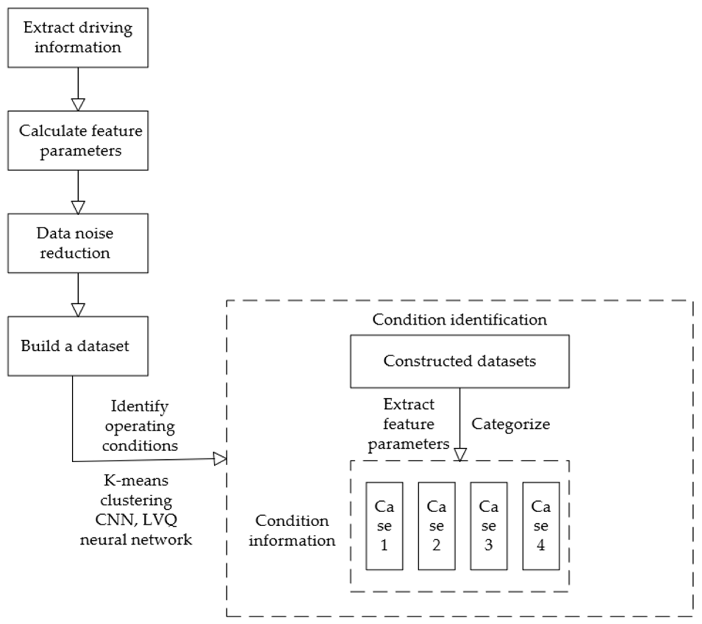
This article proposed a method for recognizing tractor conditions. This involved obtaining a tractor’s operating state information by studying the tractor’s driving speed, acceleration, angular velocity, and other real-world data. It also combined neural networks to improve the accuracy of tractor condition recognition. First, a real-world test was conducted to collect data in order to establish a data set for condition recognition. The K-means [13] clustering algorithm present in the unsupervised learning [14] algorithm was used to cluster the real-world data, outputting the cluster center, cluster category (KM-K-Means), and the distance between the sample point and the cluster center (KMD-K-Means). This resulted in four categories of conditions. A data set was established for neural network model training. Finally, the tractor condition data set was used to train on LVQ [15] and the deep learning convolutional neural network (CNN) [16] VGG-16 model. Using the VGG-16 model, an iterative optimization algorithm Relu was selected for use in up to 50 iterations in order to establish a tractor condition recognition model, and the model was evaluated using a test set. The comparative analysis of the training results of the two algorithms yielded a tractor condition recognition method that could accurately recognize the conditions of the tractor, and its management strategy is shown in Figure 1.
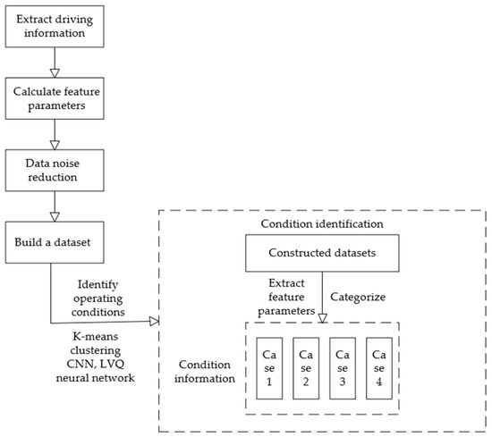
Figure 1.
Condition recognition management strategy based on neural networks.
2.1. Tractor Condition Recognition Based on One-Dimensional Convolutional Neural Networks
The most successful convolutional neural networks currently in use include the AlexNet, GoogleNet, VGG, Inception, and ResNet series, as well as other emerging lightweight networks such as capsule networks and MobileNet. Research has shown that an excessively deep CNN structure can lead to overfitting and training degradation, while an excessively shallow structure can lead to insufficient feature extraction and an inability to express deep-level information. Through the experimental comparison of the above classic structural models, the VGG-16 network with 16 weight layers was selected as the baseline structure for use in this study.
2.1.1. Algorithm Description
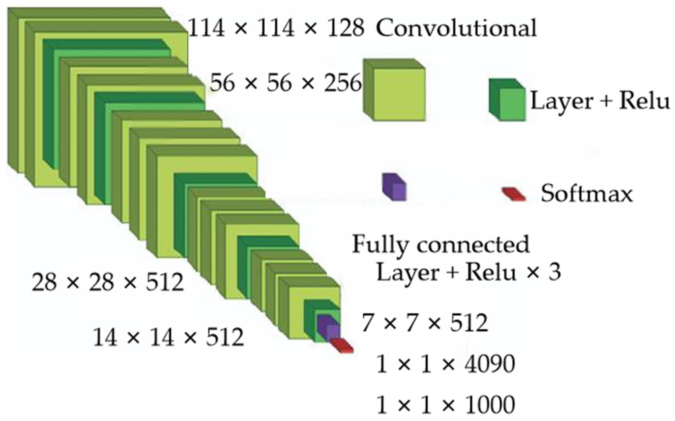
The basic structure of CNN is shown in Figure 2 [17]. It has wide applications in image classification, face recognition, audio retrieval, ECG analysis, etc. The VGG-16 model used in this article is a common CNN network structure, consisting of four layers: the convolutional layer, pooling layer, fully connected layer, and softmax classification layer. Specifically, it can be divided into five blocks, each containing several convolutional layers and one pooling layer. For example, the first block contains two convolutional layers and one pooling layer, and the fifth block contains three convolutional layers and one pooling layer. Each layer of a neural network is constructed on multiple planes composed of independently distributed neurons. The connection between layers occurs due to non-fully connected convolutional computation, and each neuron is a weighted sum of some dimensions of the input unit [18]. The width (number of channels) of the convolutional layer is 64 to 512, and the size of the convolutional kernel is mostly 3 × 3, with some convolutional kernels of size 1 × 1. This 1 × 1 convolutional kernel can be seen as a linear transformation of the input channel. At the same time, in order to improve running efficiency, a max pooling layer was constructed after some convolutional layers with a window size of 2 × 2 and a stride of 2. The first two fully connected layers each had 4096 channels, and the third fully connected layer was used for classification and had 1000 channels. The fully connected layers of all networks were configured identically, using ReLU as the activation function.

Figure 2.
VGG-16 model.
In order to make the network more applicable and improve its performance, 1000 neurons were selected for the output layer, and the softmax function was used to output the predicted classification, as shown in Equation (1), in order to calculate the probability values for each operating condition.
where is the output of the classifier’s front end output unit, c is the current category index, t is total number of categories, and is the ratio of the current element index to the sum of all element indexes, which is the probability value used to determine the current category of working condition.
2.1.2. Calculation of Recognition Accuracy
After completing model training, it is necessary to quantify the recognition accuracy using the test set. The specific formula is shown in Equation (2).
where is recognition accuracy, is the number of correct predictions for a certain type of state, and is the number of prediction errors for a certain type of state.
2.2. Tractor Condition Recognition Based on LVQ Neural Network
The classification recognition algorithms used for condition recognition include the Bayesian classification algorithm, decision tree, rough set theory, the fuzzy clustering analysis algorithm, the LVQ algorithm, support vector machine, etc. The support vector machine pattern recognition method is particularly suitable for two-dimensional problems. LVQ neural network combines competitive learning and supervised learning algorithms and has been successfully applied to pattern recognition, data compression, and other fields. Neural networks are commonly used for condition recognition problems, and so the LVQ algorithm was adopted as the method for condition recognition.
2.2.1. Algorithm Description
Neural networks are commonly used for the problem of condition recognition, and so the LVQ neural network is adopted as the method for condition recognition [19]. LVQ neural networks can be divided into LVQ1 and LVQ2 neural networks. This study adopts LVQ1 from the LVQ networks. The basic idea behind this is to determine the nearest competitive-layer neuron to the input vector and find the corresponding linear output-layer neuron connected to it. If the category of the input vector is consistent with the category corresponding to the linear output-layer neuron, then the corresponding competitive-layer neuron’s weight moves in the direction of the input vector; otherwise, if the categories are inconsistent, then the corresponding competitive-layer neuron’s weight moves in the opposite direction of the input vector.
2.2.2. Network Structure
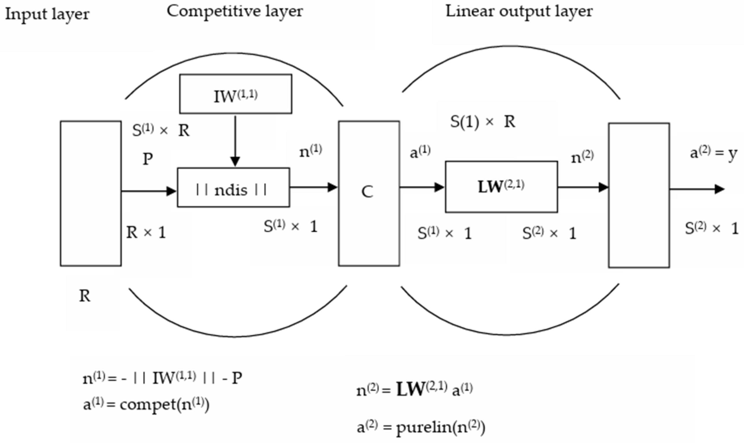
The LVQ1 neural network consists of three parts: the input layer, the competition layer, and the linear output layer. Its structure is shown in Figure 3. In the figure, P is the R-dimensional input pattern; R represents the dimension of the input training sample vector; superscript 1 and 2, respectively, represent the competition layer and the linear output layer; S is the number of neurons; n is the input of neurons; a is the output of neurons; IW(1,1) is the weight coefficient matrix between the input layer neurons and the competition layer neurons; LW(2,1) is the connection weight coefficient matrix between the competition layer neurons and the linear output-layer neurons; ||ndis|| represents the distance between two multi-dimensional vector sets; compet(·) represents the calculation processing of the competition layer neural network; and purelin(·) represents the calculation processing of the linear output-layer neural network.
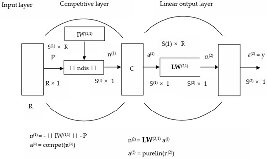
Figure 3.
LVQ neural network model.
2.3. K-Means Clustering Algorithm
2.3.1. Introduction to K-Means Clustering Algorithm
The K-means clustering algorithm is a very common, widely used, and highly representative clustering algorithm. It mainly uses distance to determine similarity, with the distance between two objects in terms of dimensional space indicating the degree of similarity between the two objects. Nodes that are closer to the cluster center form a cluster. After clustering, the best result is a compact cluster within the cluster and a dispersed cluster between the clusters [20].
2.3.2. K-Means Clustering Algorithm Process
The number of clusters k to be clustered is determined by the user, and there are 4 categories into which operating conditions are classified in this article.
We randomly selected k samples as the mean or center of the cluster, and the remaining samples were assigned to the nearest cluster based on their distance from the cluster’s center (usually assessed in terms of Euclidean distance).
It is necessary to recalculate the average value of samples within each cluster in order to form new cluster centers and repeat the process until the criterion function (see Equation (3)) converges.
where is the sum of squared errors, is the point in the space, and mi is the mean value of cluster .
It is necessary to label data: For each cluster, a label can be assigned to represent its features or meanings. For example, cluster 1 can be marked as an “accelerated start” condition, cluster 2 can be marked as a “constant speed” condition, etc. The purpose of labeling is to better understand and interpret clustering results.
3. Tractor Real-World Vehicle Data Collection and Result Analysis
3.1. Test Equipment
The experimental equipment used in this article included a Lovol tractor, an NVIDIA Jetson Nano development board, an IMU attitude sensor, a Green Union wireless projection device, and a differential GPS. The model, quantity, and function of the equipment are shown in Table 1. In Table 2, the product parameters of the Lovol tractor can be seen. Some devices are shown in Figure 4, Figure 5 and Figure 6.

Table 1.
Test equipment.
Table 2.
Tractor information.
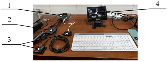
Figure 4.
Test equipment. 1—NVIDIA Jetson Nano development board; 2—Green Union wireless projection device; 3—IMU attitude sensor; 4—MAKEBIT 4B display.

Figure 5.
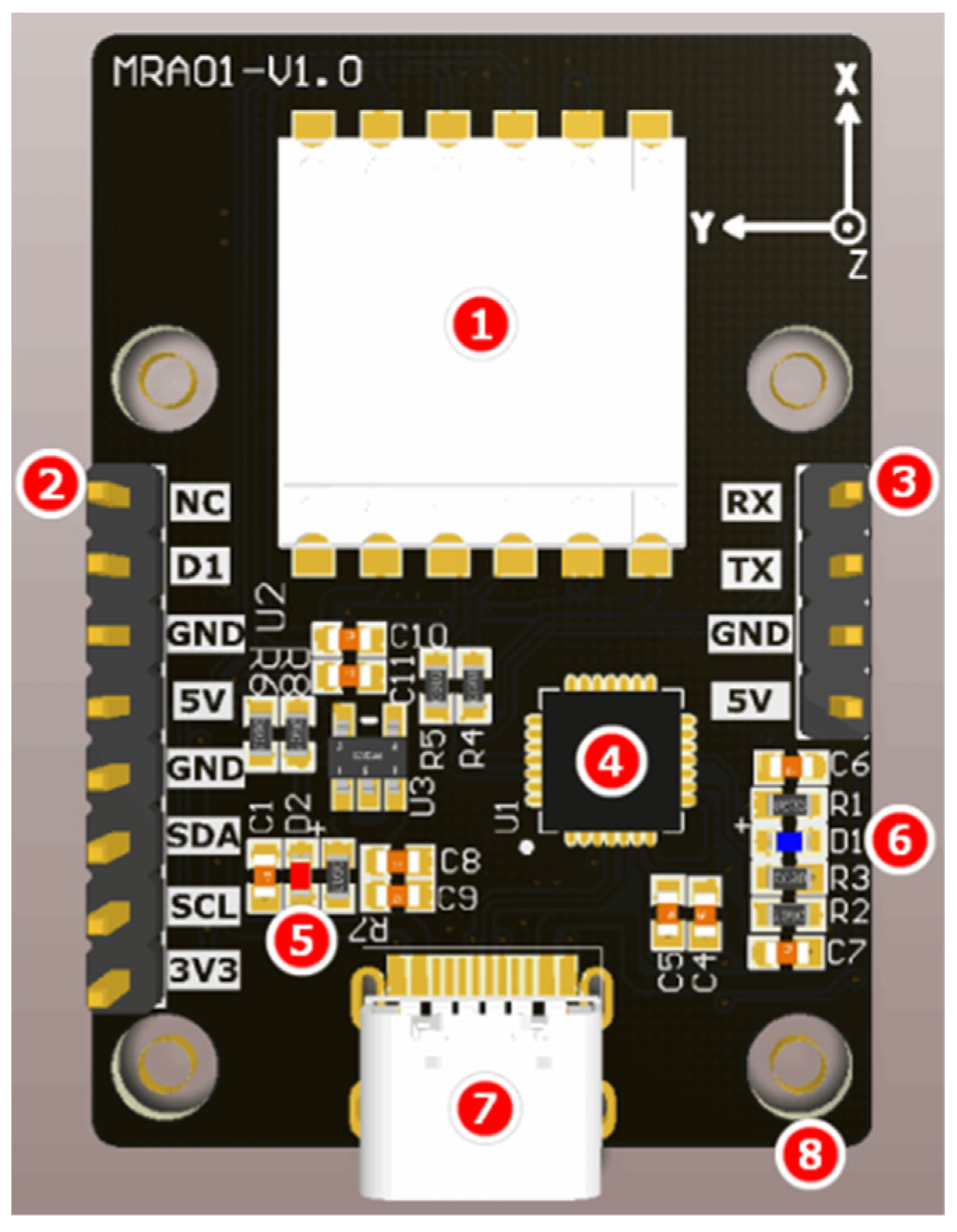
IMU. 1—the core module of the IMU module; 2—external pin; 3—serial port pin; 4—CP2102 chip; 5—D2 indicator light; 6—D1 indicator light; 7—type-C interface; 8—fixed copper pillar.
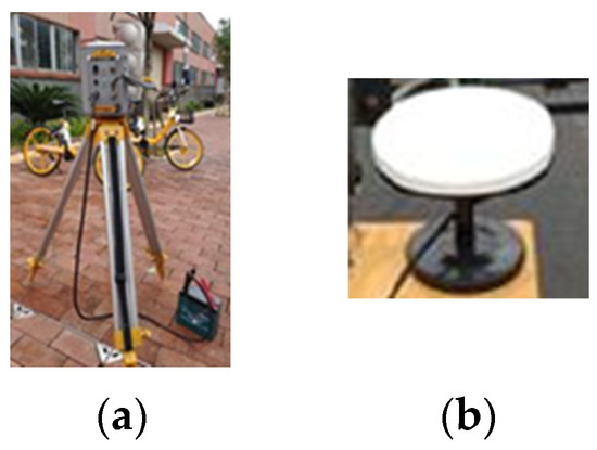
Figure 6.
Differential GPS. (a) Reference station; (b) mobile station.
3.2. Data Acquisition and Preprocessing
The data came from the actual operation records of a Lovol tractor. The data acquisition and recording software was the Vite Intelligence upper computer produced by Shenzhen Vite Intelligence Co., Ltd. (Shenzhen, China) with version number V6.2.60, and the serial port debugging assistant XCOM developed by Shenzhen Pixel Intelligence Technology Co., Ltd. (Shenzhen, China) with version number V2.6. The acquired data included the tractor’s driving speed, acceleration, angular velocity, pitch angle, roll angle, and heading angle.
In the process of constructing the condition recognition model, tractor driving data were classified and processed in practical situations, and this classification and processing could usually be directly used to construct the condition recognition model.
3.2.1. Data Acquisition
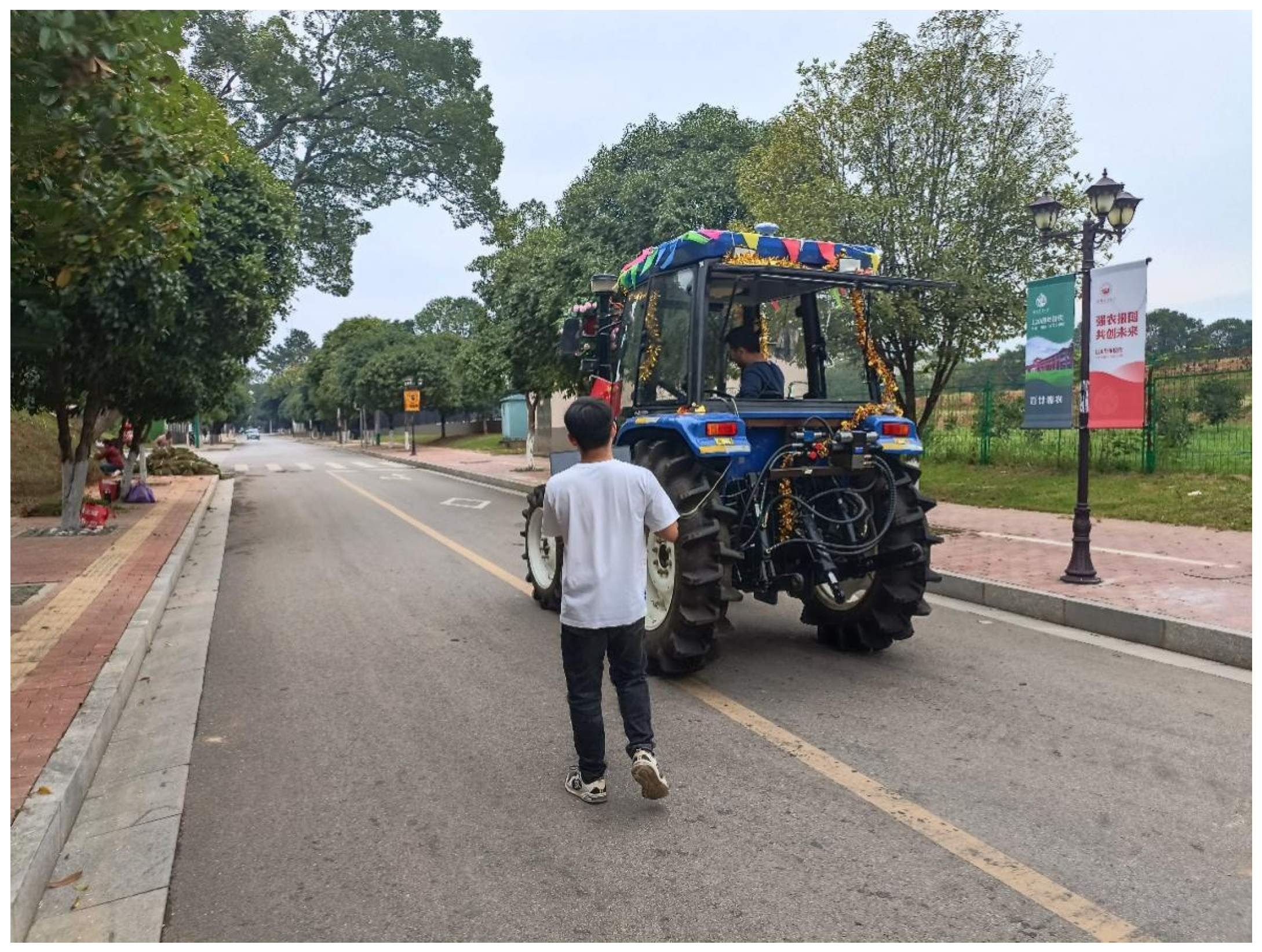
Related research shows that, if the test’s data collection time is too short, it cannot accurately include complete feature information. Conversely, if the test’s data collection time is too long, the computational burden will be too heavy under real-time control conditions [21]. To facilitate calculation and operation, the test’s time data segment needs to be changeable. The fixed distance method was used for the calculation, with a straight distance of 50 m and a turning radius of 4 m. The test was performed on 5 and 6 October 2023, and the test’s location was the experimental base of the Hunan Agricultural University. The geographical location was 111°53–114°15 E and 27°51–28°41 N. The common driving operations performed by drivers when operating tractors were straight-line forward, straight-line backward, and turning. Therefore, the test scenario was set to straight and curved roads, and the test’s implementation plan is shown in Table 3. The experimental scenario is shown in Figure 7.
Table 3.
Test Plan.

Figure 7.
Experimental scenario.
Agricultural tractors were classified into four conditions: accelerated start, constant speed, turning, and decelerated stop. The accelerated start condition (condition type “0”) referred to the intermediate state of the tractor when moving from rest to constant speed. The constant speed condition (condition type “1”) referred to the tractor maintaining a constant driving speed when moving forward or backward. The decelerated stop condition (condition type “2”) referred to the intermediate state of the tractor in terms of the constant speed condition compared to the tractor at rest. The turning condition (condition type “3”) referred to the driving state of the tractor when the steering wheel was rotated fully to the left or right under pressure from external forces when the tractor was driving at a constant speed. The driving data of the tractor were segmented into short trips, and the driving speed and other data were collected under various operating conditions in straight-line driving and turning scenarios. Some of the measured data are shown in Table 4.
Table 4.
Some measured data.
3.2.2. Data Processing
GPS differential principle is as follows: The key to differential positioning lies in eliminating GPS signal errors. GPS signals are affected by many factors during propagation, which can cause errors such as atmospheric delay clock bias, multipath effects, etc. These errors are the same for both the reference station and the mobile station when they receive the same satellite signal simultaneously. As such, by comparing the signal characteristics received by both, these errors can be accurately calculated.
There are two main ways to achieve differential positioning: real-time differential methods and post-processing differential methods. Real-time differential analysis is a method for the real-time correction of signal errors using real-time observation data from reference stations and wireless transmission with mobile stations, receiving GPS signals in real time, in order to achieve high-precision positioning. The post-processing difference refers to the method of comparing and processing the observation data of the reference station and the mobile station after data collection is completed, eliminating signal errors, and calculating the corrected position information.
IMU processes data errors based on the Kalman filtering principle, and the specific filtering process is as follows:
- Select state variables and observations;
- Construct state space equations;
- Initialize parameters;
- Substitute into the iterative formula;
- Adjust hyperparameters.
3.2.3. Feature Generation
There were 12 characteristic parameters collected during the test, as shown in Table 5. The characteristic parameters of the conditions should in principle include the characteristics of each condition. If the selection of characteristic parameters for the conditions is too large, the calculation is too large, and if the selection of characteristic parameters is too small, the unique information of each condition cannot be accurately included, resulting in large recognition errors. In order to optimize the number of characteristic parameters and ensure that each characteristic parameter independently contained the characteristic information of a certain operating condition, the tractor’s average driving speed, acceleration, angular velocity, pitch angle, roll angle, and heading angle were selected as characteristic parameters.
Table 5.
Parameters collected.
The parameter data of the specific measured characteristic are shown in Figure 8, Figure 9, Figure 10, Figure 11 and Figure 12. The values of “v”, “w”, and “a” in the following text are the composite values of velocity, angular velocity, and acceleration in the x-, y-, and z-axis directions.
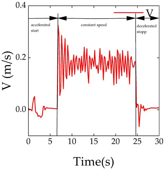
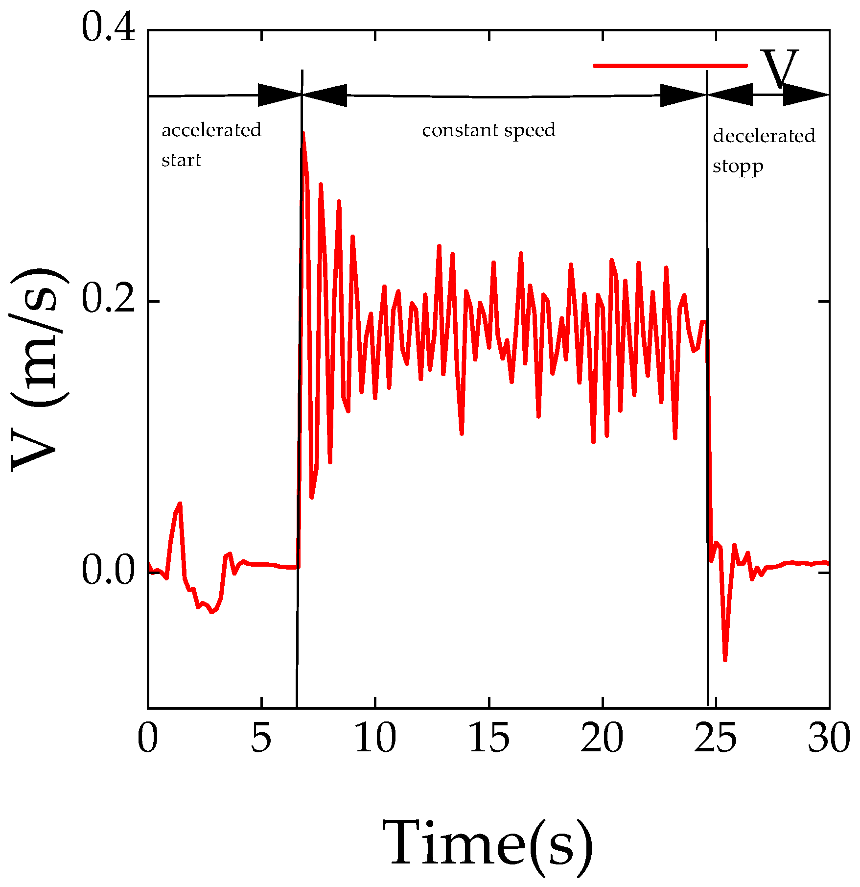
Figure 8.
Velocity curve of straight-line drive ahead.
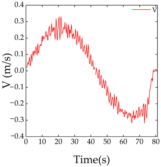
Figure 9.
Velocity curve of turn drive.
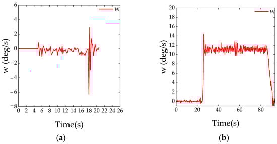
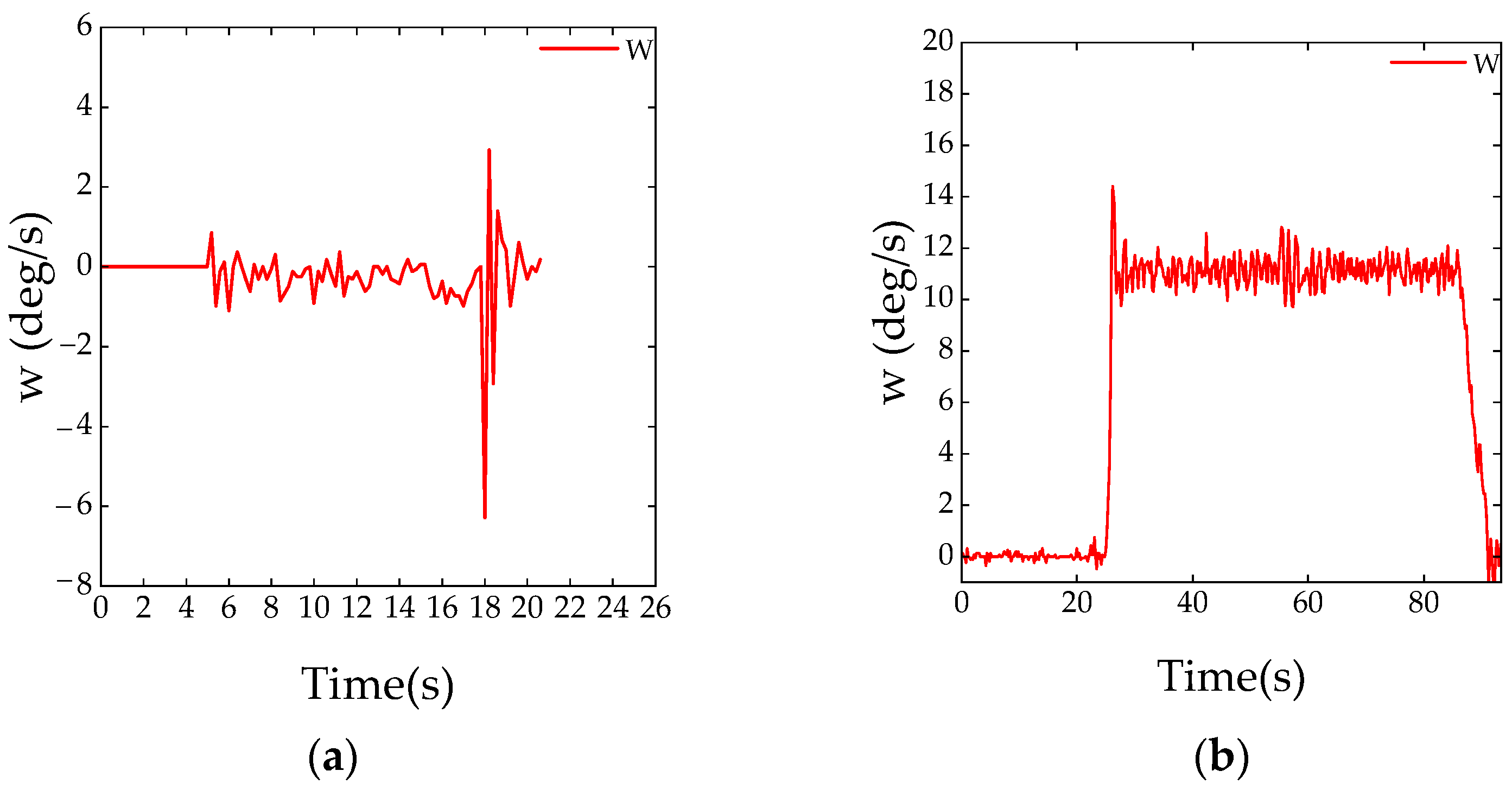
Figure 10.
Variation curve of angular velocity: (a) straight-line test scenario; (b) turn test scenario.

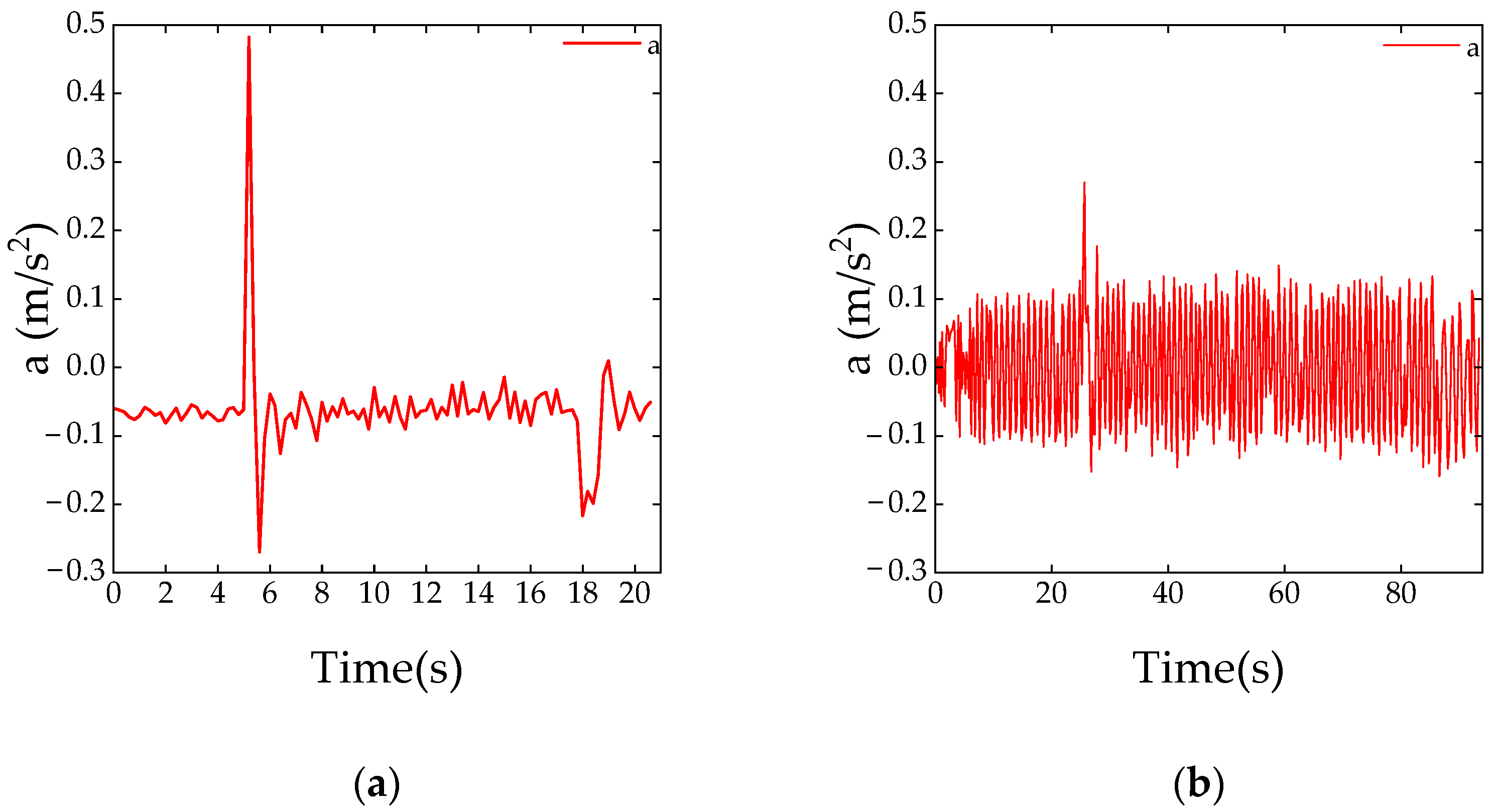
Figure 11.
Variation curve of acceleration: (a) straight-line test scenario; (b) turn test scenario.
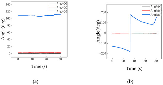
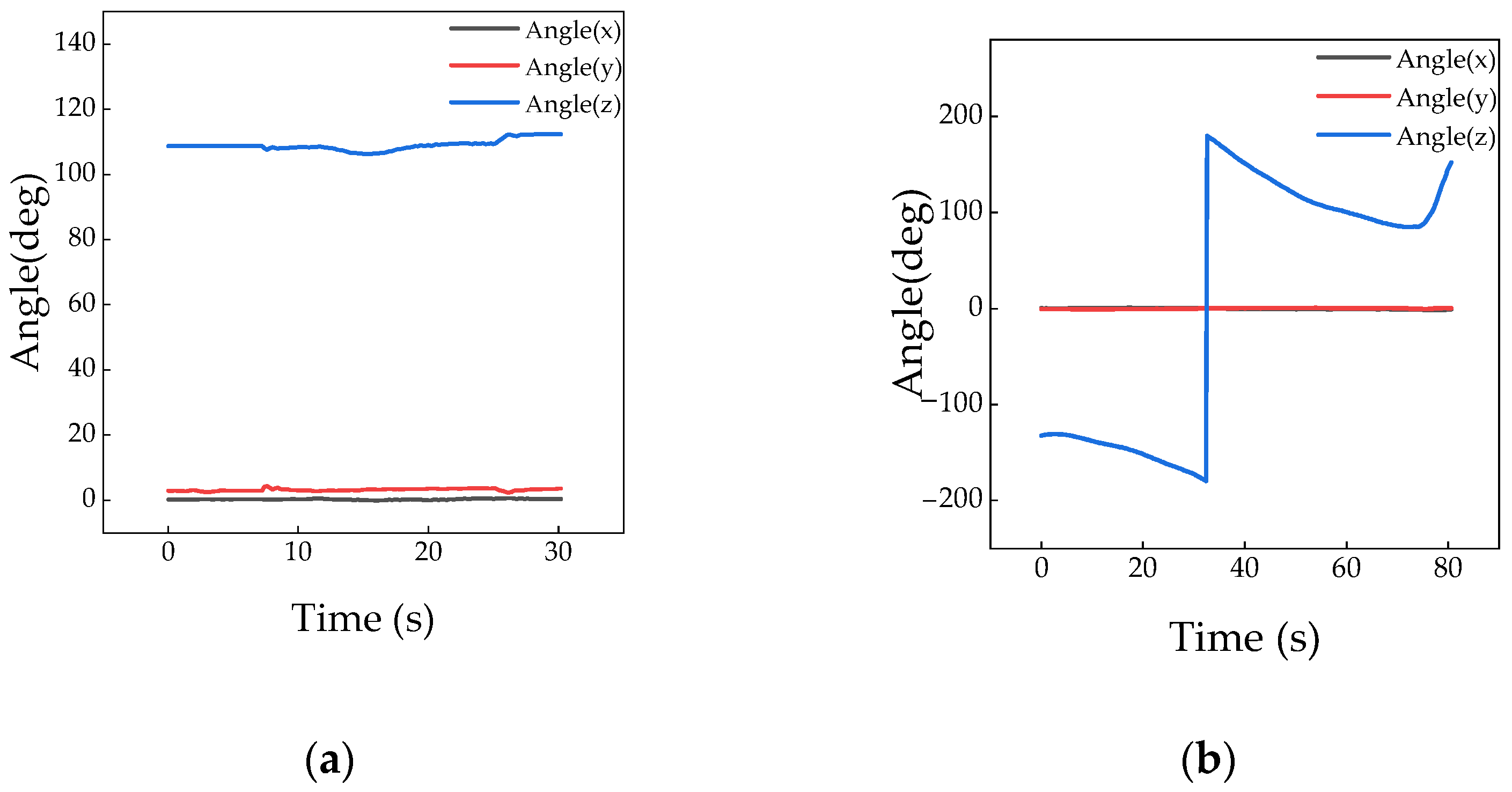
Figure 12.
Variation curve of roll, pitch, and heading angles: (a) straight-line test scenario; (b) turn test scenario.
As shown in the figure above, the change trends of six parameters, including the driving speed, acceleration, angular velocity, roll angle, pitch angle, and heading angle, were different under different conditions. During the accelerated start condition, the driving speed and acceleration changed significantly. The driving speed increased abruptly from 0 to a maximum speed of 0.32 m/s, and the acceleration approached 0.5 m/s2 at the moment of starting. After that, the tractor entered the constant speed condition, while the angular velocity did not change significantly and remained around 0 deg/s, fluctuating up and down due to errors. During the constant speed condition, the driving speed remained basically stable at 0.16 m/s, fluctuating up and down within the range of 0.06–0.28 m/s. The acceleration and angular velocity approached 0. During the decelerated stop condition, the vehicle speed decreased from 0.18 m/s to 0 m/s until the tractor stopped, and the angular velocity approached 0. The acceleration of the tractor decreased from 0 to −0.27 m/s2, and the roll angle, pitch angle, and heading angle changed in a consistent trend. The roll angle and pitch angle were both 0, and the heading angle remained at 110°. During turning, the driving speed showed a sinusoidal trend. After driving the tractor steadily, the angular velocity stabilized between by 10 deg/s and 15 deg/s, and the acceleration basically remained at 0 m/s2. The roll angle and pitch angle were both 0, and the heading angle gradually decreased between −190 deg~−110 deg when it was between 0~36 s. At 36 s, due to changes in steering angle, this increased to 195 deg, and then slowly decreased to 95 deg before stopping.
Based on the above analysis, it could be found that the tractor’s driving speed, angular velocity, acceleration, roll angle, pitch angle, and heading angle exhibited significant differences under different operating conditions. The above parameters of the tractor time-series sample points could be extracted in order to analyze and identify the tractor’s operating conditions. The recognition of tractor conditions was achieved by training neural networks to meet the requirements of subsequent related research into the precise management of a tractor’s hitching agricultural machinery.
3.2.4. Data Denoising
Noise was introduced during the generation, collection, transmission, and processing of parameter data during tractor movement. The presence of these noises posed challenges to data cleaning and analysis, as the presence of noisy data could seriously affect the results of data analysis. In machine learning tasks, noisy data could interfere with feature selection and weight allocation, thereby reducing the accuracy of the algorithm. Therefore, in terms of data processing, the following measures were taken in this article:
- Values that clearly exceeded a reasonable range were considered to be errors and deleted.
- In some cases, directly deleting noisy data may lead to information loss. As such, we employed smoothing techniques could be used to reduce the impact of noise.
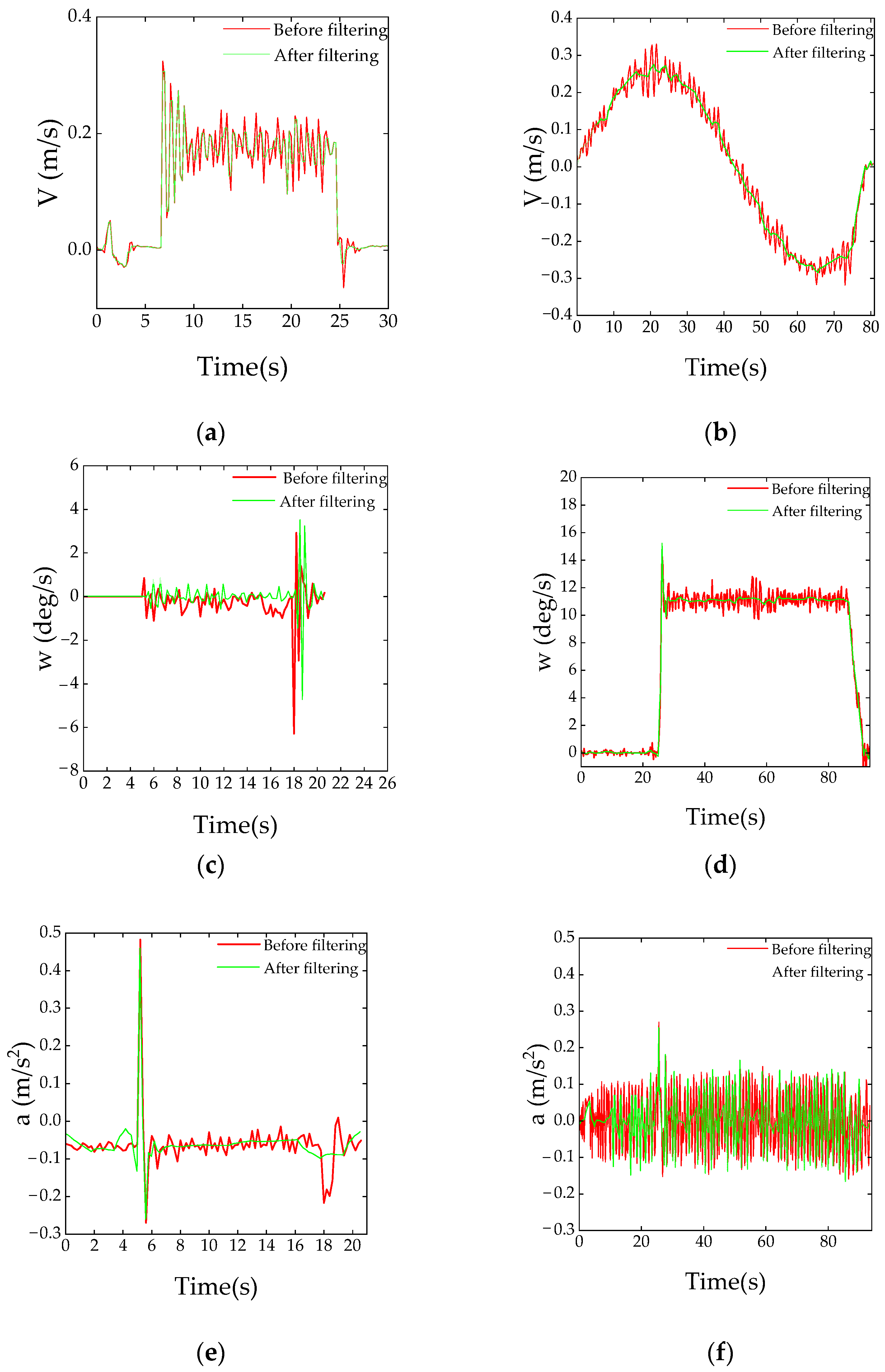
After obtaining GPS and IMU data for the various conditions of the tractor, the collected signals were denoised using the wavelet transform function in origin pro2022. Due to the relatively small amplitude of changes in roll, pitch, and heading angles during the test, only the speed, acceleration, and angular velocity were denoised in the following data. During denoising, the Daubechies wavelet function was selected as the basic function for transformation, and the wavelet transform level was 3. To process the wavelet coefficients, a soft threshold was used as the threshold type. The wavelet soft-threshold denoising method could reduce noise components in the signal, assist in the retention of important feature information, and improve signal quality. The comparisons before and after denoising are shown in Figure 13.
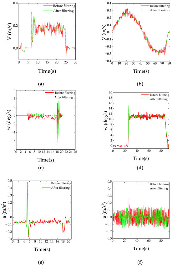
Figure 13.
Comparison of parameters before and after denoising in the data set: (a) straight-line driving speed; (b) turning driving speed; (c) straight-line driving angular velocity; (d) turning driving angular velocity; (e) straight-line driving acceleration; (f) turning driving acceleration.
The red lines shown in Figure 13a–f are the curves of driving speed and other parameters before denoising, and the green lines are the curves after denoising. It can be seen from Figure 12 that, in straight-line driving and turning scenarios, after wavelet transformation with a wavelet transform level of 3, the noise reduction effect on the parameter curves was consistent with the measured curve trend and could maximize the retention of data details and remove high-frequency signals. Compared with the denoising effect on the driving speed and angular velocity curves, the noise reduction effect on turning was more obvious, but it was still possible to determine specific conditions based on the parameter curves in straight-line driving scenarios. Comprehensively analysis of the data after denoising can be used by neural network for tractor condition recognition.
3.3. K-Means Clustering Algorithm Results
Using the SPSS STATISTIC27 tool, cluster analysis was conducted on the input parameters. After multiple analyses, the effect was better when k was set to 4.
As shown in Table 6 and Table 7, convergence was achieved due to the absence of or only slight variation in the clustering centers. The maximum absolute coordinate variation for any center was 0.000, the number of clustering iterations was 4, the minimum distance between initial centers was 55.172, and the quality of cluster cohesion and separation contour measurement was good. The clustering centers, clustering categories (KM-K-Means), and the distance between sample points and clustering centers (KMD-K-Means) were output. The four categories of conditions obtained via K-means clustering algorithm analysis were used to form a data set of conditions, completing the processing of conditions data.
Table 6.
Initial clustering centers.
Table 7.
Final clustering centers.
4. Tractor Condition Recognition Model
Neural network recognition models are based on classified samples, and the classified condition data samples need to be inserted into a prepared model. Therefore, the process of pre-processing data is crucial. According to the data pre-processing process, the existing recognition model methods can be summarized into two categories: recognition models based on measured data and recognition models based on known working conditions. This article selects the former for use constructing tractor working-condition recognition models.
4.1. Parameter Selection and Training Results of CNN VGG-16 Model
4.1.1. CNN VGG-16 Parameter Selection
In combination with the forementioned content, this article constructed a data set based on the use of tractor driving speed and acceleration information to describe the data expression of changes in tractor conditions. After K-means clustering analysis and wavelet soft-threshold denoising, the four types of condition data were input into VGG-16 CNN for training model classification. The CNN VGG-16 parameter settings are shown in Table 8, and convolutional neural networks are applied on this basis to achieve the continuous recognition of tractor conditions.
Table 8.
Parameter setting of CNN VGG-16.
We selected a data set consisting of 16 samples with a total of 4883 sample data points. Overall, 60% of the data were used as the training set, 25% were employed as the validation set for verifying the model, and the remaining 15% were used as the test set for evaluating the model. The computer configuration used for the tests was an AMD Ryzen 7 CPU with 16 GB of running memory. The PyTorch framework of PyCharm 2023 1.4 software was used to build the selected CNN VGG-16 model. The parameters were tuned on the training set with an iteration count of 50 and a learning rate of 0.1. The model dynamically adjusted the learning rate as training progressed, which better allowed for better control of the convergence speed and quality of the model and avoided overfitting and other issues. The initial weight coefficients and biases were set to random values that conformed to a normal distribution in order to improve the model’s training efficiency.
Overfitting refers to the phenomenon where machine learning models perform well on training data but perform poorly on new unseen samples. In neural network models, overfitting problems often occur. When the model overfits, this problem can be alleviated by adjusting the learning rate. In the initial stage of training, as the weights belong to a randomly initialized state, the loss function is more prone to convergence, and so a larger learning rate can be set. In the later stage of training, due to the weight approaching the optimal value, a larger learning rate cannot enable further research into the optimal value, and so a smaller learning rate is needed. The commonly used learning rate adjustment strategies include Poly, StepLR, MultiStepLR, ExponentialLR, LambdaLR, OneCycleLR, and CosineAnealingLR. CosineAnealingLR does not require hyperparameter adjustment and has high robustness, making it the preferred strategy for use improving model accuracy. Therefore, this article chooses CosineAnnexingLR as the learning rate adjustment strategy.
The VGG-16 model has the following advantages compared to other CNN models:
- Depth and simplicity. VGG16 is a convolutional neural network with a depth of 16 layers, consisting of multiple convolutional layers and fully connected layers, which helps to learn more abstract features. Its structure is relatively simple, being both easy-to-understand and implement.
- Smaller convolution kernels. VGG16 uses a small 3 × 3 convolutional kernel for feature extraction. This helps to increase the depth and non-linear expression ability of the network, while reducing the number of parameters and improving the efficiency and training speed of the model.
- Effective parameter sharing. Due to the use of convolutional kernels of the same size in the convolutional layer, VGG16 achieves parameter sharing, further reducing the number of parameters.
4.1.2. CNN VGG-16 Model Training Results
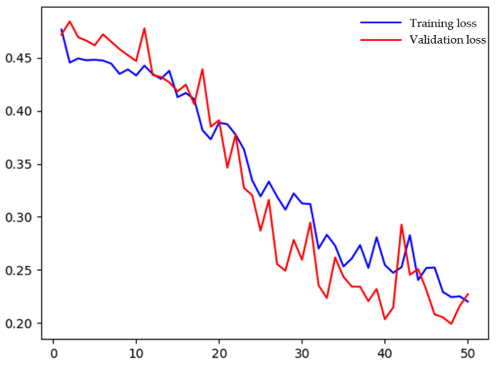
Figure 14 depicts the trend of loss values in the training and validation sets. It can be observed that, as the number of iterations increased, the model’s recognition accuracy gradually improved and stabilized at 94%. At the same time, the loss value decreased monotonically with the increase in the number of iterations, gradually approaching 0. The above analysis indicated that the model had good training performances on both the training and validation sets.
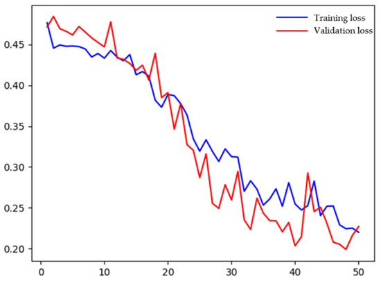
Figure 14.
Loss values of the training set and the validation set.
To further verify the reliability of the recognition model, the test set was applied to the trained model, and three indicators, including precision, recall, and F1 value (H-mean) [22], were introduced to evaluate the recognition results of the validation set and test set. The results are shown in Table 9. For the constant speed condition, all three evaluation indicators were close to 1, and the precision rate was 90.25% for the four conditions, indicating that the recognition model had high recognition accuracy and good classification performance. At the same time, by increasing the data sample size of the training set and validation set, the recognition accuracy of the model could be further improved.
Table 9.
Precision, recall, and F1 value of VGG-16 model under different conditions.
4.2. LVQ Neural Network
4.2.1. LVQ1 Neural Network Steps
The basic LVQ1 neural network steps are as follows:
Initialize the weight ωij between the input layer, the competition layer, and the learning rate η (η > 0).
Send the input vector to the input layer and calculate the distance between the neurons in the competitive layer and the input vector using Equation (4):
Select the neuron in the competitive layer closest to the input vector. If is the smallest, then the class label of the linear output-layer neuron connected to it is .
Record the class label corresponding to the input vector as . If = , adjust the weights according to Equation (5); otherwise, update the weights according to Equation (6).
4.2.2. LVQ 1 Operation and Analysis
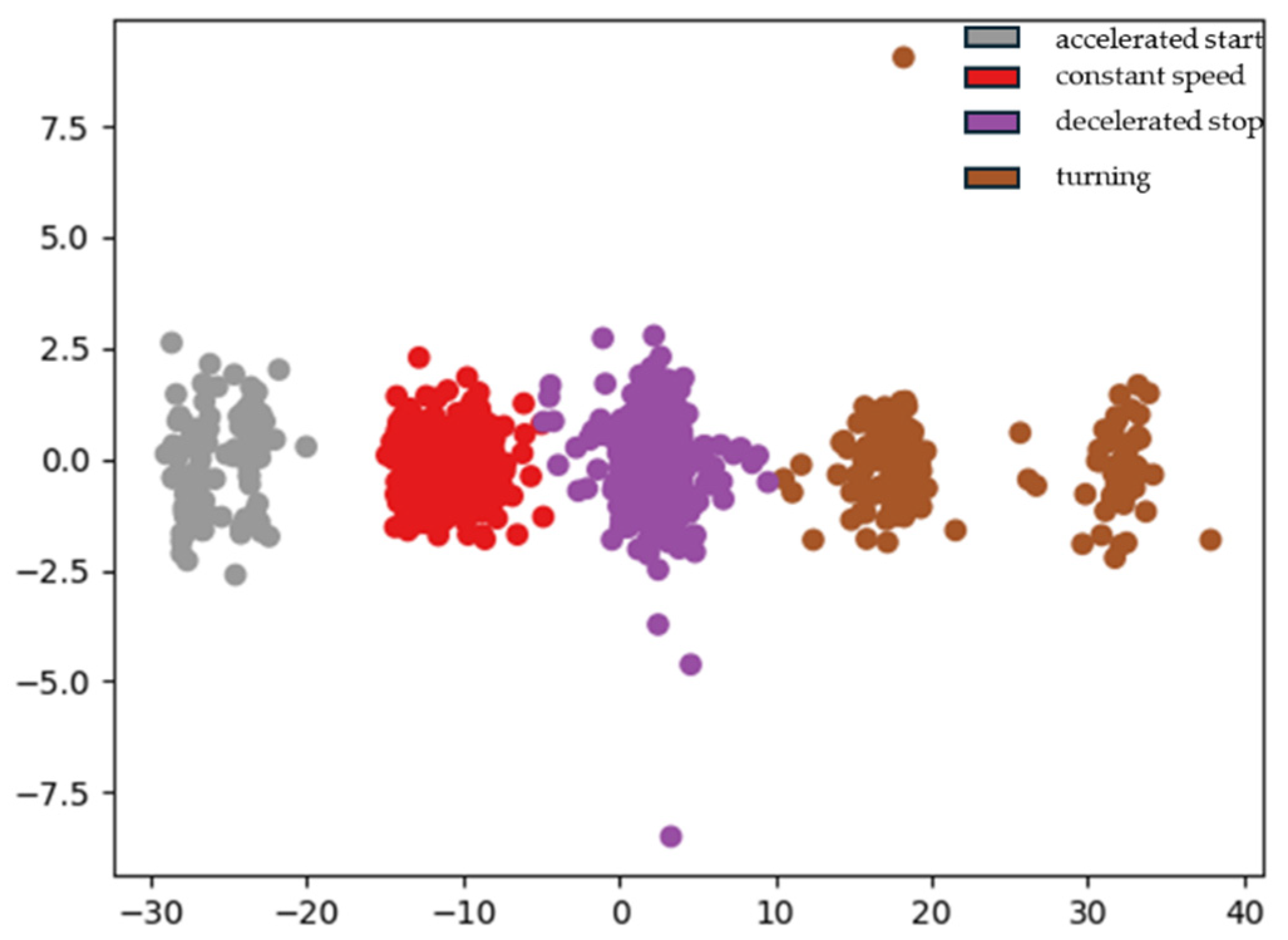
Based on the above analysis, six characteristic parameters were selected, and so the input layer of the LVQ1 neural network structure used in this study had six nodes. The competition layer classified the input vector through a competitive learning algorithm. The classes processed by the learning algorithm were called sub-classes, which were divided into clearly defined target classes. The four neurons in the linear output layer represented four tractor conditions. After 50 generations of training, the recognition error dropped to 0.01. When the recognition error stopped decreasing, the training process of the neural network algorithm was considered complete. If the samples of the prediction test set were clustered, this showed that the recognition-type judgment of the conditions established by LVQ1 neural network was correct; if the samples were dispersed, it represented that the recognition-type judgment of the conditions was incorrect. As shown in Figure 15, after training, the accuracy rate of the LVQ1 neural network model for condition recognition was 79.7%. Except for turning conditions, the LVQ1 neural network’s condition recognition model could basically assess conditions that differed in various different ways, indicating that it was feasible to use neural network techniques to recognize tractor conditions.
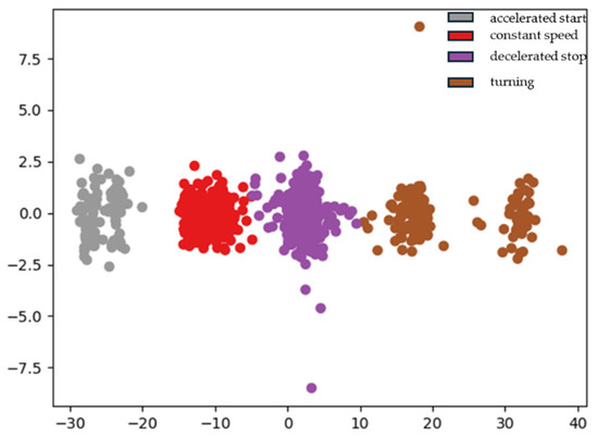
Figure 15.
LVQ1 neural network clustering result.
4.3. Discussion on the Limitations of LVQ1 Compared to CNN
LVQ neural networks, as special types of neural networks, inherit some of the advantages of neural networks, but have slow convergence speeds. LVQ1 usually requires more training cycles to converge because its learning rules are simpler and more direct than those of some other algorithms. However, it has the following drawbacks. The first is poor robustness. LVQ1 has poor robustness and may fall into local minima, especially when facing noise or nonlinear data. Further, it is difficult to effectively jump out of this local minimum. Another is insufficient accuracy. LVQ1’s classification accuracy may not be high enough, especially when dealing with non-linear, separable data sets. In fact, its performance is often inferior to that of other complex algorithms such as the BP neural network and CNN. Thirdly, the learning rate needs to be predetermined. LVQ1 requires a pre-set learning rate, and improper setting of this learning rate may lead to training failure. Unsuitable for complex pattern recognition, LVQ1 has relatively weak pattern recognition abilities and requires a high degree of quantization of input patterns. Therefore, its performance is not as good as that of some more complex neural network models when dealing with high-dimensional and complex patterns. Unable to perform continuous learning, LVQ1 does not support online learning or continuous learning, and the mode of each learning must be determined during each training period. The pattern of LVQ1 is fixed, and so it is not adapted to dynamic, changing environments or changes in data distribution. A large amount of memory is required. LVQ1 must store a weight vector for each input mode and each output mode, and so the demand for memory may be significant. In summary, although LVQ1 has the advantages of simplicity and ease of implementation, it also has obvious limitations. For complex pattern recognition tasks, more complex and powerful neural network models may be needed to replace it.
4.4. Comparison of Recognition Effects of Other Neural Networks for Conditions
The VGG-16 model has the best recognition performance among the three evaluation indicators of accuracy, recall, and F1 value, and its training time is relatively short compared to other algorithms, confirming the superiority of the CNN VGG-16 model in the field of tractor condition recognition, as shown in Table 10.
Table 10.
Comparison results.
5. Conclusions
This article used neural networks to recognize tractor conditions and employed the K-means clustering algorithm to divide the collected raw condition data samples into sets. We performed clustering analysis on the samples to obtain well-classified samples for use establishing a training set and validation set for neural networks. A condition recognition model was constructed based on the CNN algorithm and LVQ neural network, and the accuracy of the model was statistically analyzed and verified. A one-dimensional data sample was constructed using information such as tractor speed and angular velocity, and a convolutional neural network algorithm structure based on the CNN VGG-16 model was used. The data sample was iteratively optimized using the relu algorithm for up to 50 iterations, and a tractor condition recognition model was established. The model was evaluated using a test set, and it was found that the recognition accuracy of the model reached 90.25%, and the three indicators of precision, recall, and F1 value under four conditions in the test set all reached over 80%. Using the LVQ1 neural network to recognize the data sample, the accuracy reached 79.7%, indicating that both models could effectively recognize tractor conditions. However, the recognition effect of the CNN algorithm was more significant. The above condition recognition methods provide new ideas for establishing a tractor condition recognition model and provide a basis for subsequently establishing a relationship model between the tractor condition and ploughing depth detection compensation. This study uses convolutional neural network algorithms and LVQ neural network algorithms for tractor condition recognition. However, due to limitations such as data size, the structure of the condition recognition model established can be further optimized to improve recognition accuracy. Due to the limitation of sample size in the data set, there is still significant room for improvement in the accuracy of neural network models after training. In future research, we will increase the sample size to improve the accuracy of condition recognition and establish the relationship between tractor conditions and tillage depth.
Author Contributions
Conceptualization: Y.L., P.J., W.H., Y.S. and C.L.; methodology: B.L. and Y.L.; software: C.L.; site construction: C.L., W.H. and Y.S.; data curation: Y.L. and C.L.; resources: W.H. and C.L.; writing—original draft preparation: C.L.; writing—review and editing: B.L., Y.L., C.L., W.H. and P.J.; visualization: Y.L. and C.L.; supervision: Y.L., W.H. and P.J.; project administration: W.H.; funding acquisition: Y.L., W.H. and P.J. All authors have read and agreed to the published version of the manuscript.
Funding
Hunan Provincial Department of Science and Technology Major Special Projects-Top Ten Technical Research Projects (2023NK1020); Hunan Provincial Department of Science and Technology Key Area R&D Program (2023NK2010); Hunan Provincial Department of Education Key Projects (299054); Chenzhou National Sustainable Development Agenda Innovation Demonstration Zone Construction Special Project (2022SFQ20); National Key R&D Program Project (2022YFD2002001); Guangdong Agricultural Science and Technology Demonstration City Construction Fund Cooperation Project (2320060002384); Intelligent Agricultural Machinery Equipment Innovation and R&D Project of Hunan Province “R&D, Manufacturing, Promotion and Application of Green Manure Trencher in Southern Paddy Field”.
Institutional Review Board Statement
Not applicable.
Data Availability Statement
Data are contained within the article.
Conflicts of Interest
The authors declare no conflicts of interest.
References
- Fan, T.F. Exploration of the Current Situation and Development Prospects of Agricultural Mechanization in China. China S. Agric. Mach. 2021, 52, 17–18. [Google Scholar]
- Ren, H.; Wu, J.; Lin, T.; Yao, Y.; Liu, C. Research on an Intelligent Agricultural Machinery Unmanned Driving System. Agriculture 2023, 13, 1907. [Google Scholar] [CrossRef]
- Yang, Q.; Zhang, Z.; Pang, S.; Cao, H. Field vehicle position monitoring system based on GPS and GIS. Nongye Gongcheng Xuebao Trans. Chin. Soc. Agric. Eng. 2004, 20, 84–87. [Google Scholar]
- Košutić, S.; Jejčič, V.; Čopec, K.; Gospodarić, Z.; Pliestić, S. Impactof Electronic-Hydraulic Hitch Control on Rational Exploitation of Tractor in Ploughing. Strojarstvo 2008, 50, 287–294. [Google Scholar]
- Wang, P.; Meng, Z.; Yin, Y.; Fu, W.; Chen, J.; Wei, X. Automatic recognition algorithm of field operation status based on spatial track of agricultural machinery and corresponding experiment. Trans. Chin. Soc. Agric. Eng. 2015, 31, 56–61. [Google Scholar]
- Chunjiang, Z.; Xuzhang, X.C.; Yuchun, P.; Zhijun, M. Advance and prospects of precision agriculture technology system. Trans. CSAE 2003, 19, 7–12. [Google Scholar]
- Liu, Y. Research on the urban-rural integration and rural revitalization in the new era in China. Acta Geogr. Sin. 2018, 73, 637–650. [Google Scholar]
- Mei, J.; Chongyou, W.; Shuqin, H. Application and development trend of hydraulic drive and control technology in agricultural machinery. Mach. Tool Hydraul. 2017, 45, 172–176. [Google Scholar]
- Jiao, L.C.; Yang, S.Y.; Liu, F.; Wang, S.G.; Feng, Z.X. Seventy years beyond neural networks: Retrospect and prospect. Chin. J. Comput. 2016, 39, 1697–1716. [Google Scholar]
- Tian, Y.; Zhang, X.; Zhang, L. Fuzzy control strategy for hybrid electric vehicle based on neural network identification of driving conditions. Control Theory Appl. 2011, 28, 363–369. [Google Scholar]
- Wang, S.; Shi, Y.; Feng, Z.X. A method for controlling a loading system based on a fuzzy PID controller. Mech. Sci. Technol. Aerosp. Eng. 2011, 30, 166–172. [Google Scholar]
- Xu, R.; Wunsch, D. Survey of clustering algorithms. IEEE Trans. Neural Netw. 2005, 16, 645–678. [Google Scholar] [CrossRef] [PubMed]
- Ahmed, M.; Seraj, R.; Islam, S.M.S. The k-means algorithm: A comprehensive survey and performance evaluation. Electronics 2020, 9, 1295. [Google Scholar] [CrossRef]
- Yin, R.G.; Wei, S.; Li, H.; Yu, H. Introduction of unsupervised learning methods in deep learning. Comput. Syst. Appl. 2016, 25, 1–7. [Google Scholar]
- Zhang, M.; Chen, Z.; Zhou, Z. Survey on SOM algorithm, LVQ algorithm and their variants. Comput. Sci. 2002, 29, 97–100. [Google Scholar]
- Gu, J.; Wang, Z.; Kuen, J.; Ma, L.; Shahroudy, A.; Shuai, B.; Liu, T.; Wang, X.; Wang, G.; Cai, J.; et al. Recent advances in convolutional neural networks. Pattern Recognit. 2018, 77, 354–377. [Google Scholar] [CrossRef]
- Aloysius, N.; Geetha, M. A review on deep convolutional neural networks. In Proceedings of the 2017 International Conference on Communication and Signal Processing (ICCSP), Tamilnadu, India, 6–8 April 2017; pp. 588–592. [Google Scholar]
- He, K.; Ma, H.Y.; Feng, X. English handwriting identification method using an improved VGG-16 model. J. Tian Univ. 2020, 53, 984–990. [Google Scholar]
- Deng, T.; Lu, R.; Li, Y.; Lin, C. Adaptive energy control strategy of HEV based on driving cycle recognition by LVQ algorithm. China Mech. Eng. 2016, 27, 420. [Google Scholar]
- Chenxiao, G. Driving-Behavior Prediction and 22Driving-Mode Identification of Pure Electric Vehicle. Ph.D. Thesis, Dalian University of Technology, Dalian, China, 2017. [Google Scholar]
- Wang, R.; Lukic, S.M. Review of Driving Conditions Prediction and Driving Style Recognition Based Control Algorithms for Hybrid Electric Vehicles. In Proceedings of the Vehicle Power and Propulsion Conference (VPPC), Chicago, IL, USA, 6–9 September 2011; pp. 1–7. [Google Scholar]
- Kong, Q.H.; Tursun Mamat Zhao, M.J. Recognition of tractor working condition based on convolutional neural network. J. Chin. Agric. Mech. 2021, 42, 144–150. [Google Scholar]


Disclaimer/Publisher’s Note: The statements, opinions and data contained in all publications are solely those of the individual author(s) and contributor(s) and not of MDPI and/or the editor(s). MDPI and/or the editor(s) disclaim responsibility for any injury to people or property resulting from any ideas, methods, instructions or products referred to in the content. |
© 2024 by the authors. Licensee MDPI, Basel, Switzerland. This article is an open access article distributed under the terms and conditions of the Creative Commons Attribution (CC BY) license (https://creativecommons.org/licenses/by/4.0/).