BerryNet-Lite: A Lightweight Convolutional Neural Network for Strawberry Disease Identification

Abstract

With the rapid advancements in computer vision, using deep learning for strawberry disease recognition has emerged as a new trend. However, traditional identification methods heavily rely on manual discernment, consuming valuable time and imposing significant financial losses on growers. To address these challenges, this paper presents BerryNet-Lite, a lightweight network designed for precise strawberry disease identification. First, a comprehensive dataset, encompassing various strawberry diseases at different maturity levels, is curated. Second, BerryNet-Lite is proposed, utilizing transfer learning to expedite convergence through pre-training on extensive datasets. Subsequently, we introduce expansion convolution into the receptive field expansion, promoting more robust feature extraction and ensuring accurate recognition. Furthermore, we adopt the efficient channel attention (ECA) as the attention mechanism module. Additionally, we incorporate a multilayer perceptron (MLP) module to enhance the generalization capability and better capture the abstract features. Finally, we present a novel classification head design approach which effectively combines the ECA and MLP modules. Experimental results demonstrate that BerryNet-Lite achieves an impressive accuracy of 99.45%. Compared to classic networks like ResNet34, VGG16, and AlexNet, BerryNet-Lite showcases superiority across metrics, including loss value, accuracy, precision, F1-score, and parameters. It holds significant promise for applications in strawberry disease identification.

1. Introduction

Strawberries are globally adored fruits, cherished for their vibrant color, distinctive flavor, nutritional content, sweet taste, and versatility in culinary applications [1]. The strawberry crop plays a vital role in the agricultural industry as it provides delicious and nutritious fruits which are appreciated by people around the world. Nevertheless, the susceptibility of strawberries to the environment and climate factors makes them highly susceptible to a wide range of diseases. This poses significant challenges to the strawberry industry and cultivation, as these diseases can lead to a reduced yield, lower quality of fruits, and economic losses for farmers. Farmers can execute focused management techniques, which ultimately result in enhanced crop health, increased production, and lower economic losses. This is made possible by providing fast and precise disease identification. In addition, the implementation of environmentally responsible disease management strategies will contribute to the overall sustainability and environmental stewardship of strawberry production. As a result, the detection of these diseases in a timely and accurate manner is essential for the implementation of focused management strategies and the guaranteeing of the long-term viability of strawberry production.

The traditional methods for the identification of strawberry disease mainly depend on manual observation and visual examination by trained professionals [2,3,4]. Despite its familiar and widespread usage, cost-effectiveness, and suitability for experienced farmers or agricultural professionals, these methods are limited to subjectivity and human error, are time-consuming, and require expertise in disease recognition. With the advancements in artificial intelligence and computer vision, deep learning networks have become a promising solution for strawberry disease recognition. They can learn complex patterns and features from images, enabling accurate disease diagnosis [5]. However, the large and diverse dataset for training, computationally intensive during training, and the high complexity of the existing networks renders the efficient identification of strawberry diseases a formidable task [6]. Therefore, it is necessary to identify and develop a suitable method for the adaptive management of strawberry diseases.

Motivated by these challenges, in this paper, we propose BerryNet-Lite, a novel lightweight network designed for the rapid and accurate identification of strawberry diseases. We designed a lightweight model, rather than opting for a more complex, deep network architecture based on several considerations: Firstly, BerryNet-Lite requires less computational power, allowing them to run on devices without high computing capabilities, such as mobile devices or remote monitoring systems in agricultural fields. This facilitates broader deployment, especially in resource-limited environments. Secondly, although the complexity of plant disease identification demands meticulous visual analysis, BerryNet-Lite enhances processing speeds while maintaining accuracy through optimized network structures and efficient convolution operations. Additionally, rapid processing is crucial for real-time disease monitoring and timely intervention. Lastly, by employing advanced technologies like dilated convolutions and efficient channel attention (ECA) mechanisms, BerryNet-Lite effectively improves performance and generalization capabilities without significantly increasing complexity. The strength of the proposed BerryNet-Lite framework resides in its capability to provide immediate responses to strawberry diseases and pests, thereby preventing their progression to more grievous stages. Our main contributions are as follows:

(1)

We have established a comprehensive synthetic dataset which covers the various diseases of strawberries. We have carefully planned this dataset and provided a multifunctional sample set for training and testing purposes.

(2)

We designed the BerryNet-Lite framework, which combines migrant learning and expansion convolution, and finally forms a streamlined and efficient lightweight network.

(3)

We innovatively combined efficient channel attention (ECA) modules with multi-layer perception (MLP) to build a model of models. This method not only improves the recognition performance of the network, but also provides greater adaptability in the classification tasks.

(4)

We conducted extensive and comprehensive experiments. These experiments finally proved that BerryNet-Lite surpassed the existing most advanced methods on quantitative and qualitative indicators.

The rest of the paper is organized as follows: Section 2 discusses related work; Section 3 introduces the materials and methods; Section 4 conducts experimental analysis; Section 5 is the discussion; and finally, Section 6 summarizes this article.

2. Related Work

The machine learning of strawberry diseases provides an automated, efficient approach to accurately identify and classify various diseases, reducing the reliance on human resources and speeding up detection. This advancement enables agricultural producers to implement timely prevention and treatment measures, minimizing losses and boosting strawberry yield and quality. Significant advancements have already been achieved in this field.

Huang et al. [7] used computer vision to develop a machine learning method for the early detection of anthracnose in strawberries. Feldmann et al. [8] created a mathematical algorithm to classify strawberry shapes in digital images using an ordinal scale of primary principal cluster numbers. Wu et al. [9] tapped into hyperspectral imaging to detect gray mold on strawberry leaves, integrating spectral features, vegetation indices, and texture features. Mahmud et al. [10] applied machine vision for identifying powdery mildew in strawberry fields. While traditional machine vision methods have succeeded in disease detection, their reliance on manually designed features specific to strawberry diseases leads to unstable extraction and limited adaptability.

Deep learning offers a robust alternative. Li et al. [11] introduced the DAC-YOLOv4 model to detect infected strawberry leaves against complex backgrounds. Zhou [12] utilized a Mask R-CNN technique for identifying bruises on strawberries under different lighting conditions. Li et al. [13] proposed a transformer-based recognition method for strawberry disease identification. Bhujel et al. [14] developed a semantic segmentation model to detect and quantify grey mold in strawberries. Xiao et al. [15] designed a CNN-based network for identifying diseases like leaf blight, grey mold, and powdery mildew. Meanwhile, Dong et al. [16] explored an AlexNet-based method for strawberry disease classification and identification. Lee et al. [17] established a data acquisition system to amass a comprehensive dataset for training an integrated model to detect strawberry diseases. Despite these advancements, knowledge gaps remain, often presented unclearly in the literature without convincing argumentation.

Kim et al. [18] introduced a model for strawberry disease detection, suitable for integration into automated robotic systems. Anagnostis et al. [19] used a convolutional neural network to create a machine learning model for detecting leaf anthracnose disease. Ma et al. [20] proposed a recognition algorithm for strawberry diseases based on deep convolutional neural networks. Zhang et al. [21] designed the RTSD-Net model for real-time strawberry detection under field conditions. Ilyas et al. [22] identified different ripening stages of strawberries using deep learning. Yu et al. [23] developed a deep-learning-based robot for automated strawberry cultivation. Afzaal et al. [24] proposed a low-cost method for strawberry pest and disease detection using deep learning. Guo-feng et al. [25] designed a rapid disease detection method during the strawberry planting process using self-supervision. Kim et al. [26] developed a model for strawberry pest classification and detection based on deep learning. Liao et al. [27] introduced a dual-channel residual network with a multi-directional attention mechanism for detecting strawberry leaf diseases.

Jaemyung et al. [28] introduced a deep-learning method for detecting strawberry powdery mildew on leaves based on RGB images. Jiang et al. [29] utilized selected spectral features to develop a machine learning-assisted method for the early detection of anthracnose and gray mold diseases in strawberries using hyperspectral imaging. Justin et al. [30] presented a 3D deep neural network for strawberry segmentation detection using modern sensing technology. Zhou et al. [31] developed a robust structure based on Faster-RCNN improvements for detecting strawberry quality. Liu et al. [32] introduced an early detection discriminative model for strawberry anthracnose disease in indoor environments. Chen et al. [33] proposed a real-time detection model for strawberry diseases based on YOLOv5 improvements. Hu et al. [34] utilized a class activation map to locate major lesion objects and developed a lesion proposal convolutional neural network based on class attention.

In summary, significant progress has been made in strawberry disease recognition. However, certain limitations still exist:

(1)

The success of machine learning models largely depends on high-quality, well-annotated datasets. Creating comprehensive datasets is crucial, yet many studies lack access to such datasets and often rely on manually designed features specific to particular diseases. This reliance leads to unstable feature extraction when conditions change, such as variations in disease presentation or physiological changes in plants, thus limiting the robustness and scalability of the models. Training more adaptable models requires a large amount of diverse data, which is a significant bottleneck.

(2)

Although deep learning technologies offer a recognition method which does not depend on manual feature design, these models typically require a large amount of data for training. In many cases, acquiring a large-scale, well-annotated dataset of strawberry disease images is challenging, limiting the training effectiveness and ultimate performance of the models.

(3)

Another issue with deep learning models is their high demand for computational resources. The complexity of these models means that expensive hardware and considerable computing time are required for training and execution, posing a substantial barrier for resource-limited settings or implementing real-time recognition on mobile devices.

(4)

Existing methods have limited capabilities in real-time disease recognition. The rapid identification of strawberry diseases is crucial for taking timely management measures to reduce losses. However, due to the model processing speed or algorithm efficiency issues, many technologies struggle to meet the needs for real-time or near-real-time processing.

(5)

Finally, both traditional and deep learning methods have limitations in their generalization capabilities. They may perform well on specific datasets, but their performance will decline when applied to different environments or when encountering unseen disease types. This issues of overfitting or insufficient generalization limits the models’ applicability and reliability. Therefore, constructing a lightweight network has become a crucial breakthrough.

3. Materials and Methods

3.1. Data Sources

We employ a synthetic dataset comprising images of strawberry diseases, sourced from both self-collection efforts and various publicly available datasets.

Our data collection and related experiments were conducted in a strawberry field located in Xinxiang County, Henan Province, China (longitude: 113.895078, latitude: 35.231375). The actual area of the strawberry field is 5336 square meters. The experiments and data collection were conducted with the permission and authorization of the strawberry field owner. The work started on 5 March 2023, and ended around 27 December of the same year. The experiments mainly focused on the Ventana variety grown in the field. Manual photography was primarily used for data collection. Considering that some contiguous areas had dense plantations and were susceptible to damage from trampling during the concentrated ripening period, aerial photography using high-resolution imagery from drones was employed as an auxiliary method. Our related work has resulted in the creation of a comprehensive dataset on strawberry diseases. Interested readers can search for files named “Strawberry-Disease-Dataset” on GitHub and download them.

Specifically, we utilize professional-grade equipment, including the Canon camera (Canon Co., LTD. Chaoyang District, Beijing, China) and the DJIMini3 drone (Shenzhen DJI Innovation Technology Co., LTD., Nanshan District, Shenzhen City, Guangdong Province, China), to capture high-resolution images within a local strawberry orchard setting. Recognizing the scarcity of such imagery, we complement our dataset by employing web crawler techniques to gather additional images, as shown in Figure 1.

Additionally, we supplement our dataset by incorporating a select few disease datasets that are publicly accessible, as illustrated in Figure 2.

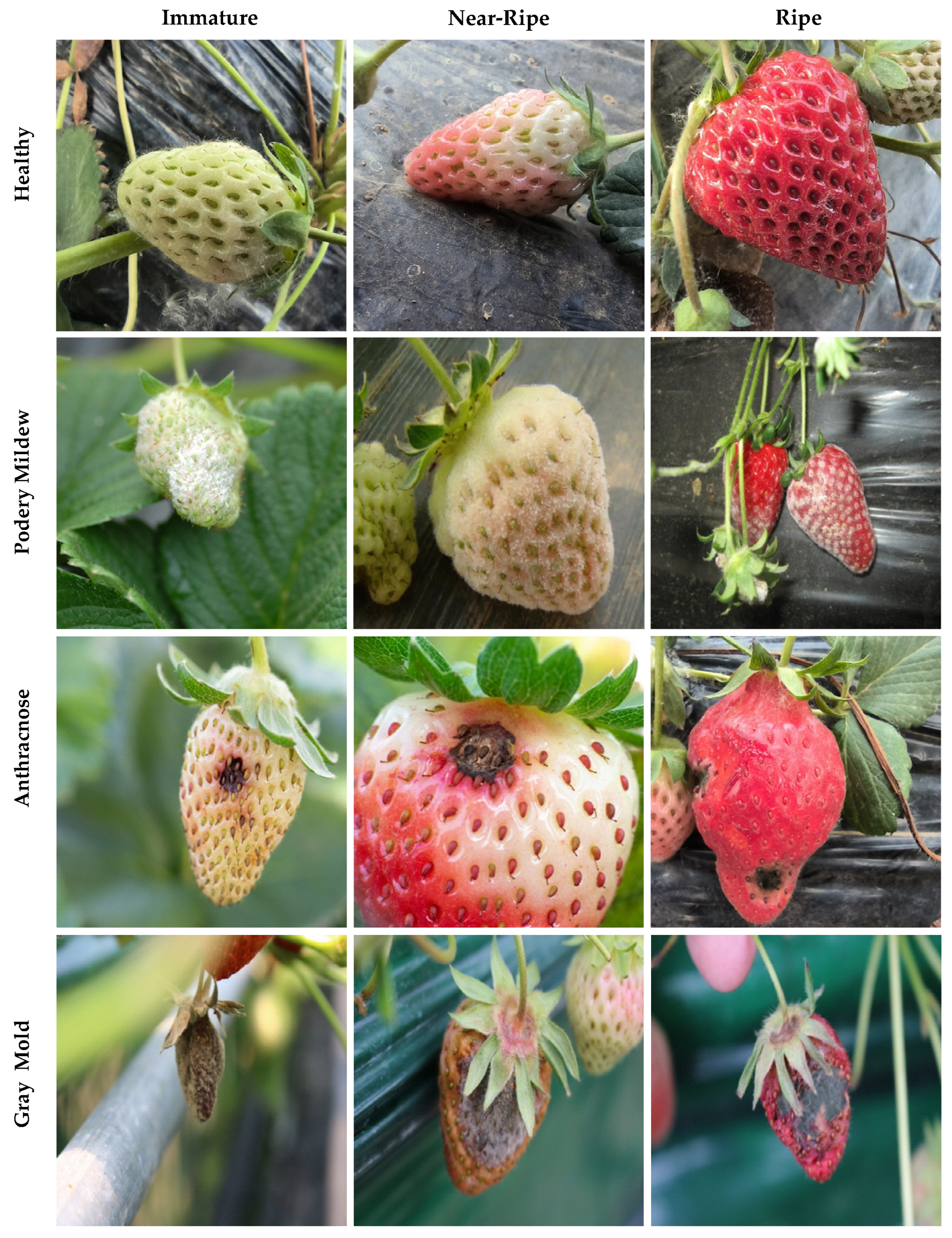
The dataset comprises three prevalent diseases at various developmental stages: powdery mildew, anthrax, and gray mold, as depicted in Figure 3.

3.1.1. Attributes of the Dataset

Due to discernible variations in feature manifestations, we delineate the primary characteristics of disease classification across different maturation stages, as shown in

Table 1. Specific descriptions for the characterization of different diseases of strawberry.

Disease Category	Feature Description
Healthy	Overall normal appearance, uniform color, usually red or normal color for the growth stage.
Powdery Mildew	White powdery appearance on the fruit surface, accompanied by an uneven fruit color and covered with a powdery substance.
Anthracnose	Black spots on the fruit surface, spreading to cause fruit rot, with colors ranging from dark brown to black.
Gray Mold	Gray fuzzy spots on the fruit surface may lead to brown soft rot, with a color ranging from gray-brown.

.

3.1.2. Data Processing Methods

This paper employs data processing techniques to optimize the strawberry disease dataset. Given the limited quantity of strawberry disease samples in real-world production and the scarcity of corresponding public datasets, data augmentation techniques are utilized to broaden the scope of the existing dataset. Specifically, this augmentation is accomplished through two methods: inversion and rotation.

Image reversal involves horizontal and vertical strategies. Horizontal reversal treats the image along the vertical axis, as shown in (1):

$$I_{horizontally}\left(x,y,z\right)=I(x_{\max }-x,y,z)$$

(1)

where $I$ represents the original image, $\left(x,y,z\right)$ denotes the original coordinates of a particular point.

Vertical reversal disposes the image along the horizontal axis, as shown in (2):

$$I_{vertically}\left(x,y,z\right)=I(x,y_{\max }-y,z)$$

(2)

Image rotation allows for clockwise or counter-clockwise rotation, simulating different image orientations. Rotation is typically represented by an angle to indicate the degree of rotation. Image rotation includes counter-clockwise rotation and clockwise rotation, as shown in (3):

$$I_{\mathrm{Rotation}}(x,y,z)=I\left(\frac{x-x_c\cos (\theta )+y_c\sin (\theta )}{\cos (\theta )},\frac{x-x_c\sin (\theta )-y_c\cos (\theta )}{\cos (\theta )},z\right)$$

(3)

where $(x_c,y_c,z_c)$ are coordinates of the rotation center, with $\theta$ denoting the angle of rotation.

During the image capture process, variations in brightness and darkness are common occurrences. Furthermore, public datasets often suffer from issues like unclear images and a lack of distinctive data features. Consequently, we enhance image quality through three approaches: contrast adjustment, chroma adjustment, and brightness adjustment. These methods are aimed at improving the visual clarity of the images, rendering them more suitable for analysis or further processing.

Contrast adjustment can enhance or reduce the brightness differences between different regions, as shown in (4):

$$I_{Contrast}\left(x,y,z\right)=P+S_{contrast}\times \left(I(x,y,z)-P\right)$$

(4)

where $P$ means the pixel value of the original image at the exact coordinates.

Chroma adjustment can enhance or reduce the color saturation of the image, playing a role in adapting to color variations under different environments. It involves adjusting the color components of each pixel in an image, as shown in (5):

$$I_{Chroma}\left(x,y,z\right)=I(x,y,z)+S_{contrast}\times \left(I(x,y,z)-G(I(x,y))\right)$$

(5)

where $G(I(x,y))$ is the grayscale value, indicating the brightness component at the exact coordinates.

The brightness adjustment can adapt images to different lighting conditions. It involves increasing or decreasing the brightness levels of all pixels in an image, as shown in (6):

$$I_{Brightness}\left(x,y,z\right)=I(x,y,z)+S_{brightness}$$

(6)

where $S$ means the enhancement factor, which is utilized to adjust the strength of image enhancement.

These techniques expand the disease dataset and widen the model’s recognition capabilities. To illustrate the effects of enhancement, we selected strawberry images, as depicted in Figure 4.

We process the disease dataset by resizing images to 224 × 224 dimensions, allowing the BerryNet-Lite model to more effectively discern image details and boost accuracy. We also leverage the Torchvision library to augment the dataset [35,36,37]. Efforts are made to normalize the classification data, balance sample distribution, minimize recognition biases, improve generalization capabilities, and prevent network overfitting. After these enhancements, the dataset is expanded to 7369 images, including 5895 in the training set and 737 each in the test and validation sets, as detailed in

Table 2. The classification data of strawberry diseases. “Original Data” represents the quantity of unprocessed data for each classification, while “Split Data” represents the quantity of processed data for each classification.

Classification	Original Data	Processed Data
Healthy	332	1874
Powdery Mildew	317	1849
Anthracnose	291	1778
Gray Mold	323	1868
All	1263	7369

.

3.2. Model of BerryNet-Lite

3.2.1. The Architecture of BerryNet-Lite

BerryNet-Lite is a lightweight neural network, integrating an inverse residual structure, a linear bottleneck layer, and squeeze-and-excitation modules. The bottleneck architecture comprises a 1 × 1 expand convolution layer, a 3 × 3 depthwise convolution layer, and a 1 × 1 projection layer. We tailored the inverse residual structure for deep separable convolution operations, enhancing efficiency. By positioning the final stage of the 1×1 expand layer outside the pooling layer, it allows the 1 × 1 layer to handle 1 × 1 feature maps directly, boosting computational speed and minimizing latency. The architecture of the network is shown in Figure 5.

In our work, we selected BerryNet-Lite as the primary model for image recognition using deep separable convolution (DSC), aiming for a balance between cost-effectiveness and performance efficiency. DSC simplifies the convolution process into two sequential operations, i.e., the depthwise convolution and pointwise convolution, optimizing the computational requirements.

At the depthwise convolution stage, a convolution operation is executed on each input channel using unique convolution kernels. Each input channel has a dedicated filter, enabling independent convolution. The tensor output of DSC is shown in (7):

$$Y_d\left(i,j,d\right)={\displaystyle {\sum }_{k=1}^K}{\displaystyle {\sum }_{l=1}^{K}X\left(i+k-1,j+l-1,d\right)\times W_d\left(k,l,d\right)}$$

(7)

where $X$ means the input feature map, $W_d\left(k,l,d\right)$ is the weight at the k-th row, l-th column, and d-th channel of the convolution kernel. The size of the kernel is $K$.

At the pointwise convolution phase, point-by-point convolution is applied to the output, aiming to achieve the integration of channels. The output tensor of the point-by-point convolution is shown in (8):

$$Y_p\left(i,j,m\right)={\displaystyle {\sum }_{d=1}^D{Y}_d\left(i,j,d\right)\times W_p\left(d,m\right)}$$

(8)

where $W_p\left(d,m\right)$ is the weight between the d and m channels of the point-by-point convolution kernel.

Ultimately, the output produced by DSC is identical to that of the pointwise convolution. The depthwise separable architecture endows BerryNet-Lite with a more streamlined form, decreasing its complexity, diminishing the risk of overfitting, and enhancing its ability to generalize. BerryNet-Lite utilizes a cross-entropy loss function to quantify the discrepancy between its output and the true labels, as detailed in (9):

$$R_{Cross-Entropy}\left(y,\overline{y}\right)=-{\displaystyle {\sum }_{i=1}^I{y}_i}\times \log \left({\overline{y}}_i\right)$$

(9)

where $I$ is the number of categories in the dataset, and $y_i$ means the code of the true label category. ${\overline{y}}_i$ is the distribution probability of the label category.

$R_{Loss}$ is the average value of the loss function for each sample $R_j$, as shown in (10):

$$R_{Loss}=\frac{1}{N}{\displaystyle {\sum }_{j=1}^N{R}_j\left(y,\overline{y}\right)}$$

(10)

where $N$ is the number of samples in the training set.

We optimize the model by minimizing the cross-entropy loss function, integrating regularization to constrain the parameters and curb the tendency towards overfitting. This approach ensures that the prediction outcomes align more closely with reality, thereby enhancing the precision.

3.2.2. Layers of BerryNet-Lite

BerryNet-Lite enhances accuracy by utilizing transfer learning, expanding its capability to generalize across a broader range and more effectively extract features after processing through expanded convolution. This efficiency is achieved by upgrading the 3 × 3 convolution to a 5 × 5 convolution.

Input Layer: This layer normalizes data dimensions and processes the raw image for initial feature extraction.

Convolutional Layer: The convolutional layers primarily consist of 3 × 3 depthwise separable convolutions and 1 × 1 pointwise convolutions, with some layers using dilation for enhanced feature extraction. Initially, a 224 × 224 image of strawberry disease is processed to extract features using 3 × 3 dilated convolutions, resizing the image to 16 × 112 × 112 while increasing the channel count to 16. This downsizing improves the model’s accuracy and reduces loss.

Pooling Layer: Pooling layers compress features to diminish the dimensions of the feature matrix while retaining essential information and spatial structure, making the model more efficient.

Fully Connected Layer: Here, features are learned comprehensively through fully connected layers, transforming feature vectors effectively. Following a fully connected layer which handles 1280 categories, a random dropout is applied to prevent overfitting. An additional fully connected layer, designed for 4 classes, is then integrated to ensure the nonlinear transformation of the model and facilitate specific disease classification. It extracts crucial classification features, supporting subsequent decision-making.

Output Layer: This layer contains as many nodes as there are categories, with each node corresponding to a classification. The SoftMax function is used to predict the probabilities for each category, based on the feature distribution of the input, facilitating accurate disease classification.

3.3. Transfer Learning and Dilated Convolution Processing

We utilized a transfer learning strategy to boost training speed, accelerate the convergence process, and improve accuracy [38]. Transfer learning leverages the relationships among different datasets and uses pre-trained parameters to train new data, effectively decreasing the number of training steps, enlarging the dataset, reducing training duration, and preventing model overfitting [39]. The process of transfer learning is illustrated in Figure 6.

Initial training was conducted using the ImageNet dataset [40]. Subsequently, we transferred the trained weights to BerryNet-Lite to enhance its generalization capabilities. During the transfer learning phase, the MLP, ECA, and expanded convolutional layers were frozen to preserve learned features.

To tackle semantic segmentation [41], dilated convolution was employed, mitigating the information loss which typically accompanies subsampling and lower resolution. By keeping the convolutional parameters constant, dilated convolution incorporates an additional parameter, known as the dilation rate, to expand the convolutional kernel’s receptive field, as illustrated in (11):

$$E{R}_i=E{R}_{i-1}+\left(k-1\right)\times S$$

(11)

where k is the size of the convolutional kernel, and S is the stride.

BerryNet-Lite enlarges the receptive field by incorporating dilated convolutions and augmenting the gaps within the convolutional kernel. Dilated convolution enables an initial 3 × 3 convolutional kernel to have an expanded receptive field, such as 5 × 5 (with a dilation rate of 2), thus avoiding down sampling [42]. Stacking multiple convolutional kernels allows dilated convolution to offer multiscale information, considering the unique receptive fields.

3.4. The Classification Head Design

3.4.1. Structure of the Classification Head

BerryNet-Lite methodically extracts features from simple to complex, with the convolutional layer identifying positional attributes of the image. After passing through the fully connected layer, it is possible to extract both global upper and lower content. Our proposed classification head design combines MLP and ECA to boost performance [43]. The MLP plays a role in identifying non-linear relationships within the channel attention framework, whereas ECA ensures efficient channel interactions using fewer parameters and less computational effort, thereby reducing the likelihood of overfitting. The classification head design of BerryNet-Lite is depicted in Figure 7.

BerryNet-Lite incorporates an MLP to boost recognition precision in complex classifications. The layer averages perceptions and captures the full distribution of input features, revealing intricate details that could otherwise be overlooked. The non-linear activation layer, utilizing the rectified linear unit (ReLU), enhances the representational power of features. Thanks to the MLP’s relatively few parameters, the overall model size remains manageable, thus improving recognition accuracy and the ability to generalize.

Additionally, it utilizes the ECA module, which includes an average pooling layer, a 1 × 1 convolutional layer, and a sigmoid activation function [44]. This module adopts a focused, local cross-channel interaction strategy to gather inter-channel interaction insights [45]. By incorporating ECA, BerryNet-Lite effectively maintains dimensional integrity, boosting performance with a minimal increase in parameters.

3.4.2. The Average Perception Learning Algorithm for MLP

BerryNet-Lite prioritizes a lightweight structure in contrast to traditional MLPs, which are hindered by large parameter sizes and high computational complexity, challenging efficient inference on resource-limited devices [46]. To overcome these limitations, we introduce the average perception learning (APL) algorithm, designed to enhance MLP efficiency by decreasing both the number of parameters and the computational load.

In the algorithm, it initializes the weight vector $f$, and the learning rate $z$ in the perception to 0. Subsequently, the training samples are randomly accessed in sequential order. For each sample $(x_n,y_n)$, $f$ is used to predict the classification ${\widehat{y}}_n$. The difference between the expected sample and the actual sample is calculated $y_n-{\widehat{y}}_n$. If a classification error occurs, $f$ and $z$ are updated based on the difference value, as shown in (12) and (13):

$$f_{i+1}=f_i+z\times (y_n-{\widehat{y}}_n)\times x_n$$

(12)

$$z_{i+1}=z_i+1$$

(13)

After the updates are completed, the iteration count $g$ is incremented by 1. If $g$ reaches the maximum iteration count $g_{\max }$, the update loop terminates. Otherwise, it continues to access the next sample, repeating the updating process. After the APL ends, to counteract the impact of the random order, a final averaging is applied to the last weight vector $f$.

The final output yields the parameter $F$ of the averaged perception model, as shown in (14):

$$F=\frac{f}{g_{\max }}=\frac{f_i+f_{i-1}}{g+1}$$

(14)

The APL algorithm iteratively refines the perception model by leveraging training samples from the strawberry disease dataset [47]. Its objective is to progressively converge upon and identify the most effective parameter settings, thereby reducing classification errors. The pseudocode of is shown in Algorithm 1:

Algorithm 1. The APL algorithm
1:	$\mathbf{Input}: F_{IN}={\left\{\left(x_i^g,y_i^g\right)\right\}}_{g_i=1}^{g_{\max }}$; //input the training set, the maximum number of generations is g
2:	$\mathbf{Initialize}: f_i=0$$; z_i=0$$, g_i=0$; //initialize weight vector
3:	$\mathbf{for} (i=0,i<g_{\max },i++$)
4:	$F_{IN}^{New}\leftarrow Ran{d}_{O\mathrm{rder}}\left(F_{IN}\right)$; //Randomly order the samples in training set F;
5:	$\left\{x_i^{New},y_i^{New}\right\}\leftarrow Extract\left(F_{IN}^{New}\right)$; //Sample extraction
6:	${\widehat{y}}_i^g\leftarrow Predict\left(y_i^{New}\right)$; //Predicting sample
7:	$\mathbf{if} (g_i<g_{\max }$){
8:	$f_{i+1}=f_i+z_i\times \left(y_i^g-{\widehat{y}}_i^g\right)x_i^g$; //Updating the weight vector
9:	$z_{i+1}=z_i+1$; //Updating the learning rate
10:	$g_{i+1}=g_i+1$; //Calculate the number of iterations
11:	$F_{OUT}^{New}=\frac{f_{i+1}}{g_{i+1}}$; //Calculate the output result
12:	else
13:	continue;
14:	endif
15:	$F_{OUT}\leftarrow F_{OUT}^{New}$;
16:	end for
17:	$\mathbf{Output}: F_{OUT}$

3.4.3. The Feature Fusion Algorithm Based on ECA and MLP

ECA effectively enhances channel interactions, while MLP excels at identifying nonlinear relationships between channels. By integrating both, we transcend the constraints of conventional feature fusion techniques, enabling a more thorough capture and use of information from input data, thus augmenting the model’s ability to represent data. BerryNet-Lite incorporates MLP to improve feature utilization and employs ECA to capture global correlations, targeting a significant boost in overall performance. The coefficients employed by the MLP module are detailed in (15):

$$h_{MLP\left(x\right)}=\sigma \left(W_2\times R\left(W_1\times x+b_1\right)+b_2\right)$$

(15)

where $x$ represents the input feature, $W$ and $b$ denotes the weight matrix and bias in terms of the corresponding layer, and $\sigma$ is the activation function. The coefficients utilized by the ECA module are shown in (16):

$$h_{ECA\left(x\right)}=\sigma \left(\beta \times \phi \left(x\right)+\upsilon \right)$$

(16)

where $\beta$ and $\phi$ are the learned vectors, while $\upsilon$ is the attention weight.

We use $h_{MLP(x)}$ and $h_{ECA(x)}$ to represent the overall features extracted by MLP and ECA, respectively. Since each feature interprets the same disease differently, some features may pinpoint the disease accurately, while others might cause significant misinterpretations or lead to unclear classification outcomes [48]. To address this, we implement a multi-layer network fusion mechanism at the output end of each feature network, applying targeted enhancement or suppression to each original output feature. Subsequently, dot product fusion aggregates these features, enabling a collaborative process that boosts recognition performance. The dual-feature fusion methodology comprises three key components: weighted addition, dot product fusion, and multilayer feature output, detailed in (17):

$$h_{Cov}\left(x\right)=\left({\displaystyle \sum _{i=1}^m{\lambda }_i{h}_{MLP\left(x\right)}^i+1}\right)+\left({\displaystyle \sum _{j=1}^n{\mu }_j{h}_{ECA\left(x\right)}^j+1}\right)$$

(17)

Weighted addition introduces trainable weights, $\lambda$ and $\mu$, to each element of the features. These weights are applied to the original outputs to either amplify or diminish the model’s recognition abilities [49]. The weighted outputs are then combined to produce a scalar value, which quantifies the neural network model’s effectiveness based on this weighted multiplication. Dot product fusion executes a dot product operation on the aggregated feature weights derived from the preceding step. This process leverages multiple sets of dot product fusion results in the multilayer feature output as the ultimate fusion output. The abundance of fusion result sets correlates directly with a more robust representation of the recognition capacity. Within the dual-stream fusion framework [50], features extracted through the multilayer perception and attention mechanisms are fed into the BerryNet-Lite model. The feature fusion is conducted as specified in (17), subsequently linking to the fully connected layer for the classification task. The procedure of the feature fusion algorithm is shown in Algorithm 2:

Algorithm 2. Feature fusion algorithm
1:	Input: $F_i\left(x\right)$ //Strawberry disease data
2:	for $\left(i=1;i\le n;i++\right)$
3:	$Q_{\mathrm{disease}}\left[ \right]\leftarrow Frame\left(F_i\left(x\right)\right)$//Data set framing based on the disease
4:	if (is-disease-recognized)
5:	$MLP\left(x\right)\leftarrow {{\displaystyle \sigma }}_{graphic\_anchor}({{\displaystyle Q}}_{disease}[ ])$ //Mark the MLP module feature
6:	$ECA\left(x\right)\leftarrow {{\displaystyle \sigma }}_{(channel\times graphic)\_anchor}({{\displaystyle Q}}_{disease}[ ])$ //Mark the attention module feature
7:	$Identify\left(MLP(x)\&ECA(x)\right)$ //Determine confidence graph, channel, frame
8:	$h_{MLP\left(x\right)}\leftarrow MLP\left(M\mathrm{atrix}\left(h_{MLP(x)}^i\right)\right)$ //MLP characteristic training
9:	$h_{ECA\left(x\right)}\leftarrow ECA\left(M\mathrm{atrix}\left(h_{ECA(x)}^j\right)\right)$//ECA feature training
10:	$Co{v}_{MLP(x)}\leftarrow h_{MLP\left(x\right)}+1$//MLP feature convolution processing
11:	$Co{v}_{ECA(x)}\leftarrow h_{ECA\left(x\right)}+1$//Attention channel feature convolution processing
12:	$h_{Cov}\left(t\right)=Co{v}_{MLP(x)}+Co{v}_{ECA(x)}$//Feature convolution fusion
13:	else
14:	continue
15:	endif
16:	end for
17:	Output $h_{Cov}\left(x\right)$//Output fusion feature

4. Results

We utilized Python 3.7 and CUDA 11.6 within the PyCharm 2022 to build our model, operating on a 64-bit CentOS Linux 7 OS. The hardware setup included an Intel Xeon(R) Gold 6248R CPU and a Tesla V100S PCIE 32 GB GPU. We extensively used the PyTorch framework and the Torchvision library, along with other image processing tools. This feature allowed for the real-time construction, modification, and debugging of our model, facilitating the development of an efficient strawberry disease recognition system. The specific parameter settings are detailed in

Table 3. BerryNet-lite model parameter settings.

Parameter Name	Value	Parameter Name	Value
Data_size	224 × 224	Dropout	0.2
Momentum	0.9	Loss Function	Cross Entropy
Epoch	120	Depthwise Separable Layer	15
Learning Rate	0.001	Conv layer	18
Batch_size	8	Conv Kernel	3 × 3, 5 × 5
Height_stride	1	Feature Dimension	1024
Width_stride	1	Inverted Residual Block Activation Function	H-Swish
Optimizer	AdamW	Hidden Layer Activation Function	ReLU

.

4.1. Evaluation Indicators

On the strawberry disease dataset, we evaluated the performance of BerryNet-Lite using metrics such as recall, precision, loss value, accuracy, and F1 score. The term “true positive” (TP) refers to the count of samples where the actual positive instances are correctly identified as positive. “False negative” (FN) signifies the instances where positive cases are mistakenly classified as negative. “False positive” (FP) is used for instances where negative cases are wrongly labeled as positive. “True negative” (TN) denotes the instances where negative cases are accurately classified as negative.

Accuracy serves as a metric for gauging a classification model’s performance, indicating the ratio of correctly predicted samples by the model to the overall sample count. This is depicted in (18):

$$Accuracy=\frac{TP+TN}{TP+TN+FP+FN}$$

(18)

Precision is a metric used to measure the accuracy of a classification model, reflecting the percentage of samples correctly identified as positive out of all the samples predicted to be positive by the model, as illustrated in (19):

$$Precision=\frac{TP}{TP+FP}$$

(19)

Recall, also referred to as the Sensitivity or True Positive Rate, is a performance metric for classification models. It quantifies the percentage of true positive samples accurately identified by the model out of all actual positive cases, as detailed in (20):

$$Recall=\frac{TP}{TP+FN}$$

(20)

The F1 Score is a metric which merges precision and recall, offering a comprehensive evaluation of performance. It calculates the harmonic mean of precision and recall, serving to evaluate the model’s positive predictive value alongside its capability to accurately identify positive cases, as shown in (21):

$$F1=\frac{2Precision\times Recall}{Precision+Recall}$$

(21)

The value of the loss function primarily reflects the disparity between the number of correctly identified samples and the total number of samples, as demonstrated in (22):

$$Loss=\frac{-1}{n}\times {\displaystyle \sum (\alpha \times \log h_{\alpha \_hat}+(1-\alpha )\times \log (1-h_{\alpha \_hat}))}$$

(22)

where $n$ denotes the total number of samples, $h_{\alpha \_hat}$ represents prediction for the positive class, $\alpha$ denotes the ground truth, and log is the natural logarithm function.

4.2. Ablation Experiment

BerryNet-Lite consists of the basic network module (BerryNet), core components such as ECA and MLP, and key technologies including transfer learning (TL) and dilated convolution (DC). To assess the importance of each part of BerryNet-Lite, we conducted ablation studies.

Through ablation experiments, the efficacy of BerryNet-Lite is further validated. Under identical conditions, the enhanced modules are sequentially incorporated, and the values of various metrics are utilized to demonstrate the performance at different improvement stages. The results are shown in Figure 8.

The experiments demonstrate that the introduction of transfer learning significantly improved the model’s accuracy from 94.5% to 98.2% while reducing the loss value from 0.2441 to 0.1261. Following the incorporation of ECA, a notable acceleration in the convergence speed was observed, along with a 0.46% increase in accuracy. Furthermore, the application of dilated convolution boosted the model’s accuracy to 99.08%. Finally, through the integration of the MLP module, it achieved a final accuracy of 99.45%, accompanied by a reduction in the loss value to 0.0905. The results of ablation experiments are presented in

Table 4. Results of ablation experiments that presents the optimal training outcomes of the model across different metrics.

Method	Loss	Accuracy (%)	Precision (%)	Recall (%)	F1 (%)
BerryNet	0.2441	94.47	92.70	95.98	94.30
BerryNet + TL	0.1261	98.16	96.51	93.09	94.76
BerryNet + TL + ECA	0.1458	98.62	97.37	93.96	95.64
BerryNet + TL + ECA + DC	0.1409	99.08	97.87	95.83	96.84
BerryNet + TL + ECA + DC + MLP (BerryNet-Lite)	0.0905	99.45	97.96	97.91	96.90

.

In transfer learning, applying the method to a task different from the original one introduces distinct features to the feature extractor of BerryNet, resulting in a decrease in the recall rate. However, upon integrating ECA as an attention mechanism, the model demonstrates a significant improvement in both accuracy and precision. Compared to BerryNet, the accuracy and precision notably increase by 4.15% and 4.67%, respectively. Subsequent methods, such as dilated convolution and the addition of an MLP, show a certain degree of improvement in mitigating this phenomenon induced by transfer learning.

Finally, integrating all the improvement methods into BerryNet results in a decrease of 0.1536 in the loss value and increases of 4.98%, 5.26%, 1.93%, and 2.6% in accuracy, precision, recall, and F1 score, respectively. Thus, by combining the enhancements from the aforementioned methods, the recognition performance of the BerryNet-Lite model for strawberry disease has been optimized compared to the original model.

4.3. Generalization Experiment

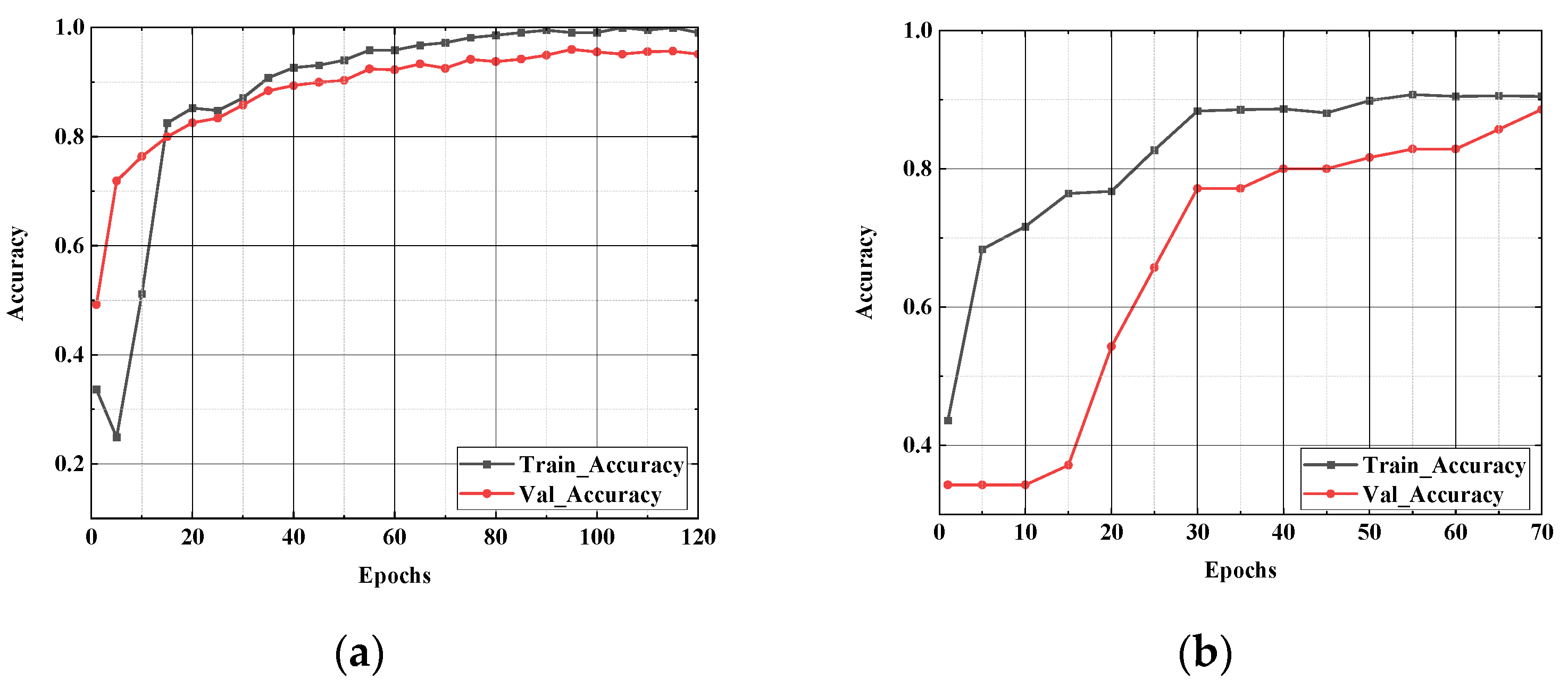
To evaluate the generalization capability of the BerryNet-Lite model, we conducted a comparative analysis of accuracy and loss rates across the training and testing sets of the strawberry disease dataset. This experiment involved a dataset consisting of 506 images, including 137 images of regular strawberries, 125 images of powdery mildew, 113 images of anthracnose, and 131 images of gray mold. The training set, which accounted for 80% of the total dataset, comprised 406 images sourced from our self-constructed dataset. The remaining 10% of the dataset, comprising 50 images, was utilized as the testing and validation set. The results are shown in Figure 9.

The curves of the training and validation sets demonstrate that the model swiftly converges on the strawberry disease dataset with minimal fluctuations. In contrast, the curve on the dataset constructed for this experiment exhibits more pronounced volatility compared to the original dataset. Nevertheless, the accuracy of the BerryNet-Lite model increases with the number of training iterations on both datasets. The loss values on both training and testing sets are illustrated in Figure 10.

4.4. Classification Experiment

In this work, the gradient-weighted class activation mapping (Grad-CAM) technique was applied, directing arbitrary target gradients into the final convolutional layer to generate a coarse localization map [51]. This map emphasizes crucial areas leveraged by the model for predictions. Utilizing Grad-CAM, a feature attention visualization heatmap was produced, vividly showcasing the feature extraction process and highlighting nuanced details within image features. Figure 11 displays the resulting heatmap, offering a visual insight into the model’s predictive focus.

Image analysis reveals that diseased portions of strawberries are characterized by darkness and emitted brightness, along with unusual colors that signify performance in specific areas. The intensity of focus on these regions is symbolized by the color red. Following the integration of the ECA mechanism, the BerryNet-Lite model shows increased attention to the features related to strawberry disease during the feature extraction process [52]. The visualization heatmap, produced through this technique, further supports effectiveness in classifying and identifying strawberry diseases.

This study conducts an independent verification of the model’s accuracy in classifying strawberries into four categories: healthy, powdery mildew, anthracnose, and gray mold, utilizing the strawberry disease validation set. The Python code is used to produce the validation results. In the outcomes generated, “class” refers to the name of the specific disease classification, and “prob” indicates the accuracy of the refined model in each respective classification. These validation outcomes offer vital insights into the model’s performance and its ability to classify diseases, aiding in a more comprehensive evaluation and enhancement of the model. The specific results are illustrated in Figure 12.

4.5. Comparative Experiment

Comparative experiments are specifically designed to assess and compare the performance of distinct models. In this paper, we utilize the strawberry disease dataset to compute the performance of BerryNet-Lite model. We train both widely recognized models and the BerryNet-Lite model across several measures to highlight the superior performance of the proposed model.

To further establish BerryNet-Lite’s predominance, it is benchmarked against five other models: AlexNet [53], VGG16 [54], ResNet34 [55], MobileNetV2 [56], and MobileNetV3 [57]. The reconfigurations of these parameters are delineated in

Table 5. Comparison of network parameters.

Network	Parameters	Value
AlexNet	Hidden layer	3
	Conv layer	5
	Max-pooling layer	2
	Conv kernel	3 × 3, 5 × 5, 11 × 11
	Feature dimension	4096
	LRN Layer	5
ResNet34	Hidden layers	28
	Conv layer	34
	Max-pooling layer	4
	Conv kernel	1 × 1, 3 × 3, 7 × 7
	Feature dimension	2048
	Residual connections layer	2
VGG16	Hidden layers	3
	Conv layer	16
	Max-pooling layer	5
	Conv kernel	3 × 3
	Feature dimension	4096
MobileNetV2	Depthwise separable layer	20
	Conv layer	30
	Conv kernel	3 × 3
	Feature dimension	1280
MobileNetV3	Depthwise separable layer	15
	Conv layer	20
	Conv kernel	3 × 3
	Feature dimension	1024

.

AlexNet and VGG16 possess complex architectures with numerous convolutional and fully connected layers, tailored for extensive image classification tasks. Conversely, BerryNet-Lite is designed with a focus on lightweight structures, optimizing it for environments limited by computational resources. ResNet34 introduces a novel approach with its residual blocks and skip connections, ensuring seamless information flow across layers—a distinct difference from BerryNet-Lite’s application of depthwise separable convolution. MobileNetV3 incorporates the SE attention mechanism, offering a contrast in feature extraction efficiency to BerryNet-Lite’s implementation of the ECA attention mechanism. MobileNetV2, a precursor to MobileNetV3, also adopts depthwise separable convolution, but relies on ReLU for activation. Each model brings unique attributes to the table, demonstrating remarkable capabilities in various settings. The performance of these models, in terms of accuracy and loss on the strawberry disease dataset, is illustrated in Figure 13.

The graph above demonstrates that BerryNet-Lite consistently outperforms other models on the strawberry disease dataset, achieving higher accuracy and lower loss values. A thorough comparison of crucial metrics, including loss, accuracy, precision, F1 score, and model parameters, is provided in a tabular format in

Table 6. Comparison of Different Models. The table presents the optimal training outcomes of the model across different metrics.

Method	Loss	Accuracy (%)	Precision (%)	Recall (%)	F1 (%)	Params
AlexNet	0.1511	98.35	94.55	98.08	96.28	14.59 M
ResNet34	0.1398	98.90	98.21	96.49	97.34	21.80 M
VGG16	0.2350	96.70	96.76	96.74	96.74	134.28 M
MobileNetV2	0.2065	97.25	92.16	97.92	94.95	3.47 M
MobileNetV3	0.2441	96.77	92.70	95.98	94.31	2.54 M
BerryNet-Lite	0.1261	99.45	97.96	97.91	97.93	2.87 M

.

The comparative data accentuates BerryNet-Lite’s pronounced advantage in terms of parameter count, with only 2.87 million parameters, thereby underscoring the merits of lightweight neural network design. Despite a slight dip in precision relative to ResNet34 and a lower recall compared to MobileNetV2 and AlexNet, its F1 score surpasses all other models assessed. This discrepancy highlights BerryNet-Lite’s superior overall performance capability.

In summary, BerryNet-Lite distinguishes itself through high accuracy, parameter efficiency, and comprehensive performance excellence. Minor disparities in specific evaluation metrics with other models do not significantly detract from its overarching efficacy in strawberry disease detection. The following confusion matrix, resulting from disease classification efforts, illustrates both the precision and the challenges in accurately identifying individual diseases by BerryNet-Lite, alongside comparisons with MobileNetV3, MobileNetV2, ResNet34, VGG16, and AlexNet.

The confusion matrix, as depicted in Figure 14, outlines the recognition results, with rows indicating predicted categories and columns showing actual categories. Diagonal elements represent the likelihood of accurately identifying disease classifications, while off-diagonal elements reflect the chances of misclassification. The confusion matrix demonstrates that BerryNet-Lite achieves greater accuracy in identifying diverse disease classifications compared to other models. This observation strongly supports the efficacy of BerryNet-Lite in strawberry disease recognition.

5. Discussion

This study introduces BerryNet-Lite, a convolutional neural network tailored for the precise identification of strawberry diseases. Given the scarcity of publicly available datasets for such specialized applications, we meticulously crafted a comprehensive disease dataset, covering various growth stages of strawberries for thorough experimental validation. BerryNet-Lite minimizes the reliance on expensive computing resources with its automated feature extraction and lightweight network design.

For the classification head design, ECA and MLP modules are integrated. These modules significantly enhance the model’s ability to identify subtle differences in strawberry diseases, especially when dealing with visually similar symptoms. The ECA module adjusts channel weights of convolutional layer outputs, enhancing the model’s focus on key features in images. This channel-level attention mechanism enables the model to more precisely pinpoint disease features, improving diagnostic accuracy even in visually similar disease states. Additionally, the MLP module, as a fully connected network layer, performs nonlinear transformations after feature fusion, enhancing the model’s learning capacity from raw inputs to final outputs. This nonlinear processing of deep features is crucial for distinguishing subtle differences between complex disease progression stages and similar symptoms. Through the combination of ECA and MLP, the BerryNet-Lite model not only improves overall accuracy in strawberry disease recognition, but also enhances its ability to differentiate between disease types and stages which are visually challenging to distinguish. This technological innovation provides robust support for achieving rapid and accurate monitoring and management of strawberry diseases.

However, BerryNet-Lite also has limitations. For example, the training and testing primarily rely on datasets collected from specific regions, potentially affecting its applicability and effectiveness in different global regions. Additionally, while the model generally exhibits good recognition ability for most strawberry diseases, further validation of its performance is needed for identifying certain rare or specific disease stages.

6. Conclusions

This paper introduces BerryNet-Lite, a lightweight neural network for the precise identification of various strawberry diseases. Utilizing a comprehensive dataset encompassing strawberries at different maturity levels and afflicted with a range of diseases, the model employs transfer learning to accelerate convergence speed via pre-training and integrates dilated convolution to enhance the accuracy of feature extraction. Additionally, it incorporates the efficient channel attention (ECA) mechanism to establish an attention module and develops a multi-layer perception (MLP) algorithm to improve generalization capability and capture the abstract features of diseases. A novel classification head design, combining ECA and MLP, has also been implemented. Extensive experiments have demonstrated the efficiency and effectiveness of BerryNet-Lite in the domain of strawberry disease recognition, benefiting from its innovative approach which merges multiple perception modules, dilated convolution, and lightweight attention mechanisms. This synergy reduces model complexity while enhancing performance metrics such as accuracy, recall, and precision, and lowering loss rates.

This paper provides a novel tool for the efficient recognition of strawberry diseases, and opens new avenues for utilizing deep learning technology to improve disease identification in agriculture. Moving forward, BerryNet-Lite is set to be applied to a wider range of crop diseases, aiding in the automation and intelligent management of agricultural production. Future research should prioritize enhancing the resilience and adaptability of disease recognition models under varying environmental conditions, lighting conditions, and disease severities.

References

- Wang, B.; Li, H.; You, J.; Chen, X.; Yuan, X.; Feng, X. Fusing Deep Learning Features of Triplet Leaf Image Patterns to Boost Soybean Cultivar Identification. Comput. Electron. Agric. 2022, 197, 106914. [Google Scholar] [CrossRef]
- Yang, B.; Wang, Z.; Guo, J.; Guo, L.; Liang, Q.; Zeng, Q.; Zhao, R.; Wang, J.; Li, C. Identifying Plant Disease and Severity from Leaves: A Deep Multitask Learning Framework Using Triple-Branch Swin Transformer and Deep Supervision. Comput. Electron. Agric. 2023, 209, 107809. [Google Scholar] [CrossRef]
- Wang, X.; Pan, T.; Qu, J.; Sun, Y.; Miao, L.; Zhao, Z.; Li, Y.; Zhang, Z.; Zhao, H.; Hu, Z.; et al. Diagnosis of Soybean Bacterial Blight Progress Stage Based on Deep Learning in the Context of Data-Deficient. Comput. Electron. Agric. 2023, 212, 108170. [Google Scholar] [CrossRef]
- Shahi, T.B.; Sitaula, C.; Neupane, A.; Guo, W. Fruit Classification Using Attention-Based MobileNetV2 for Industrial Applications. PLoS ONE 2022, 17, e0264586. [Google Scholar] [CrossRef]
- Li, L.; Zhang, S.; Wang, B. Apple Leaf Disease Identification with a Small and Imbalanced Dataset Based on Lightweight Convolutional Networks. Sensors 2021, 22, 173. [Google Scholar] [CrossRef]
- Lanjewar, M.G.; Panchbhai, K.G. Convolutional Neural Network Based Tea Leaf Disease Prediction System on Smart Phone Using Paas Cloud. Neural Comput. Appl. 2023, 35, 2755–2771. [Google Scholar] [CrossRef]
- Huang, S.; Du, Y.; Jin, Y.; Wang, J.; An, W. Computer Vision-Based Anthrax Detection System for Strawberry. Int. Core J. Eng. 2022, 8, 837–846. [Google Scholar]
- Feldmann, M.J.; Hardigan, M.A.; Famula, R.A.; Lopez, C.M.; Tabb, A.; Cole, G.S.; Knapp, S.J. Multi-Dimensional Machine Learning Approaches for Fruit Shape Phenotyping in Strawberry. GigaScience 2020, 9, giaa030. [Google Scholar] [CrossRef] [PubMed]
- Wu, G.; Fang, Y.; Jiang, Q.; Cui, M.; Li, N.; Ou, Y.; Diao, Z.; Zhang, B. Early Identification of Strawberry Leaves Disease Utilizing Hyperspectral Imaging Combing with Spectral Features, Multiple Vegetation Indices and Textural Features. Comput. Electron. Agric. 2023, 204, 107553. [Google Scholar] [CrossRef]
- Mahmud, M.S.; Zaman, Q.U.; Esau, T.J.; Price, G.W.; Prithiviraj, B. Development of an Artificial Cloud Lighting Condition System Using Machine Vision for Strawberry Powdery Mildew Disease Detection. Comput. Electron. Agric. 2019, 158, 219–225. [Google Scholar] [CrossRef]
- Li, Y.; Wang, J.; Wu, H.; Yu, Y.; Sun, H.; Zhang, H. Detection of Powdery Mildew on Strawberry Leaves Based on DAC-YOLOv4 Model. Comput. Electron. Agric. 2022, 202, 107418. [Google Scholar] [CrossRef]
- Zhou, X.; Ampatzidis, Y.; Lee, W.S.; Zhou, C.; Agehara, S.; Schueller, J.K. Deep Learning-Based Postharvest Strawberry Bruise Detection under UV and Incandescent Light. Comput. Electron. Agric. 2022, 202, 107389. [Google Scholar] [CrossRef]
- Li, G.; Jiao, L.; Chen, P.; Liu, K.; Wang, R.; Dong, S.; Kang, C. Spatial Convolutional Self-Attention-Based Transformer Module for Strawberry Disease Identification under Complex Background. Comput. Electron. Agric. 2023, 212, 108121. [Google Scholar] [CrossRef]
- Bhujel, A.; Khan, F.; Basak, J.K.; Jaihuni, M.; Sihalath, T.; Moon, B.-E.; Park, J.; Kim, H.-T. Detection of Gray Mold Disease and Its Severity on Strawberry Using Deep Learning Networks. J. Plant Dis. Prot. 2022, 129, 579–592. [Google Scholar] [CrossRef]
- Xiao, J.-R.; Chung, P.-C.; Wu, H.-Y.; Phan, Q.-H.; Yeh, J.-L.A.; Hou, M.T.-K. Detection of Strawberry Diseases Using a Convolutional Neural Network. Plants 2020, 10, 31. [Google Scholar] [CrossRef] [PubMed]
- Dong, C.; Zhang, Z.; Yue, J.; Zhou, L. Automatic Recognition of Strawberry Diseases and Pests Using Convolutional Neural Network. Smart Agric. Technol. 2021, 1, 100009. [Google Scholar] [CrossRef]
- Lee, S.; Arora, A.S.; Yun, C.M. Detecting Strawberry Diseases and Pest Infections in the Very Early Stage with an Ensemble Deep-Learning Model. Front. Plant Sci. 2022, 13, 991134. [Google Scholar] [CrossRef] [PubMed]
- Kim, B.; Han, Y.-K.; Park, J.-H.; Lee, J. Improved Vision-Based Detection of Strawberry Diseases Using a Deep Neural Network. Front. Plant Sci. 2021, 11, 559172. [Google Scholar] [CrossRef] [PubMed]
- Anagnostis, A.; Asiminari, G.; Papageorgiou, E.; Bochtis, D. A Convolutional Neural Networks Based Method for Anthracnose Infected Walnut Tree Leaves Identification. Appl. Sci. 2020, 10, 469. [Google Scholar] [CrossRef]
- Ma, L.; Guo, X.; Zhao, S.; Yin, D.; Fu, Y.; Duan, P.; Wang, B.; Zhang, L. Algorithm of Strawberry Disease Recognition Based on Deep Convolutional Neural Network. Complexity 2021, 2021, 6683255. [Google Scholar] [CrossRef]
- Zhang, Y.; Yu, J.; Chen, Y.; Yang, W.; Zhang, W.; He, Y. Real-Time Strawberry Detection Using Deep Neural Networks on Embedded System (Rtsd-Net): An Edge AI Application. Comput. Electron. Agric. 2022, 192, 106586. [Google Scholar] [CrossRef]
- Ilyas, T.; Khan, A.; Umraiz, M.; Jeong, Y.; Kim, H. Multi-Scale Context Aggregation for Strawberry Fruit Recognition and Disease Phenotyping. IEEE Access 2021, 9, 124491–124504. [Google Scholar] [CrossRef]
- Yu, Y.; Zhang, K.; Liu, H.; Yang, L.; Zhang, D. Real-Time Visual Localization of the Picking Points for a Ridge-Planting Strawberry Harvesting Robot. IEEE Access 2020, 8, 116556–116568. [Google Scholar] [CrossRef]
- Afzaal, U.; Bhattarai, B.; Pandeya, Y.R.; Lee, J. An Instance Segmentation Model for Strawberry Diseases Based on Mask R-CNN. Sensors 2021, 21, 6565. [Google Scholar] [CrossRef]
- Yang, G.; Yang, Y.; He, Z.; Zhang, X.; He, Y. A Rapid, Low-Cost Deep Learning System to Classify Strawberry Disease Based on Cloud Service. J. Integr. Agric. 2022, 21, 460–473. [Google Scholar]
- Kim, H.; Kim, D. Deep-Learning-Based Strawberry Leaf Pest Classification for Sustainable Smart Farms. Sustainability 2023, 15, 7931. [Google Scholar] [CrossRef]
- Liao, T.; Yang, R.; Zhao, P.; Zhou, W.; He, M.; Li, L. MDAM-DRNet: Dual Channel Residual Network with Multi-Directional Attention Mechanism in Strawberry Leaf Diseases Detection. Front. Plant Sci. 2022, 13, 869524. [Google Scholar] [CrossRef] [PubMed]
- Shin, J.; Chang, Y.K.; Heung, B.; Nguyen-Quang, T.; Price, G.W.; Al-Mallahi, A. A Deep Learning Approach for RGB Image-Based Powdery Mildew Disease Detection on Strawberry Leaves. Comput. Electron. Agric. 2021, 183, 106042. [Google Scholar] [CrossRef]
- Jiang, Q.; Wu, G.; Tian, C.; Li, N.; Yang, H.; Bai, Y.; Zhang, B. Hyperspectral Imaging for Early Identification of Strawberry Leaves Diseases with Machine Learning and Spectral Fingerprint Features. Infrared Phys. Technol. 2021, 118, 103898. [Google Scholar] [CrossRef]
- Le Louëdec, J.; Cielniak, G. 3D Shape Sensing and Deep Learning-Based Segmentation of Strawberries. Comput. Electron. Agric. 2021, 190, 106374. [Google Scholar] [CrossRef]
- Zhou, C.; Hu, J.; Xu, Z.; Yue, J.; Ye, H.; Yang, G. A Novel Greenhouse-Based System for the Detection and Plumpness Assessment of Strawberry Using an Improved Deep Learning Technique. Front. Plant Sci. 2020, 11, 559. [Google Scholar] [CrossRef] [PubMed]
- Liu, C.; Cao, Y.; Wu, E.; Yang, R.; Xu, H.; Qiao, Y. A Discriminative Model for Early Detection of Anthracnose in Strawberry Plants Based on Hyperspectral Imaging Technology. Remote Sens. 2023, 15, 4640. [Google Scholar] [CrossRef]
- Chen, S.; Liao, Y.; Lin, F.; Huang, B. An Improved Lightweight YOLOv5 Algorithm for Detecting Strawberry Diseases. IEEE Access 2023, 11, 54080–54092. [Google Scholar] [CrossRef]
- Hu, X.; Wang, R.; Du, J.; Hu, Y.; Jiao, L.; Xu, T. Class-Attention-Based Lesion Proposal Convolutional Neural Network for Strawberry Diseases Identification. Front. Plant Sci. 2023, 14, 1091600. [Google Scholar] [CrossRef] [PubMed]
- Bi, C.; Xu, S.; Hu, N.; Zhang, S.; Zhu, Z.; Yu, H. Identification Method of Corn Leaf Disease Based on Improved Mobilenetv3 Model. Agronomy 2023, 13, 300. [Google Scholar] [CrossRef]
- Gao, G.; Wang, C.; Wang, J.; Lv, Y.; Li, Q.; Ma, Y.; Zhang, X.; Li, Z.; Chen, G. CNN-Bi-LSTM: A Complex Environment-Oriented Cattle Behavior Classification Network Based on the Fusion of CNN and Bi-LSTM. Sensors 2023, 23, 7714. [Google Scholar] [CrossRef] [PubMed]
- Wang, J.; Zhang, X.; Gao, G.; Lv, Y.; Li, Q.; Li, Z.; Wang, C.; Chen, G. Open Pose Mask R-CNN Network for Individual Cattle Recognition. IEEE Access 2023, 11, 113752–113768. [Google Scholar] [CrossRef]
- Cao, B.; Zhang, B.; Zheng, W.; Zhou, J.; Lin, Y.; Chen, Y. Real-Time, Highly Accurate Robotic Grasp Detection Utilizing Transfer Learning for Robots Manipulating Fragile Fruits with Widely Variable Sizes and Shapes. Comput. Electron. Agric. 2022, 200, 107254. [Google Scholar] [CrossRef]
- Jin, X.; Xiong, J.; Rao, Y.; Zhang, T.; Ba, W.; Gu, S.; Zhang, X.; Lu, J. TranNas-NirCR: A Method for Improving the Diagnosis of Asymptomatic Wheat Scab with Transfer Learning and Neural Architecture Search. Comput. Electron. Agric. 2023, 213, 108271. [Google Scholar] [CrossRef]
- Mahmud, M.S.; He, L.; Zahid, A.; Heinemann, P.; Choi, D.; Krawczyk, G.; Zhu, H. Detection and Infected Area Segmentation of Apple Fire Blight Using Image Processing and Deep Transfer Learning for Site-Specific Management. Comput. Electron. Agric. 2023, 209, 107862. [Google Scholar] [CrossRef]
- Sun, J.; Zhou, J.; He, Y.; Jia, H.; Liang, Z. RL-DeepLabv3+: A Lightweight Rice Lodging Semantic Segmentation Model for Unmanned Rice Harvester. Comput. Electron. Agric. 2023, 209, 107823. [Google Scholar] [CrossRef]
- Zhang, S.; Zhang, S.; Zhang, C.; Wang, X.; Shi, Y. Cucumber Leaf Disease Identification with Global Pooling Dilated Convolutional Neural Network. Comput. Electron. Agric. 2019, 162, 422–430. [Google Scholar] [CrossRef]
- Zhang, Y.; Ma, B.; Hu, Y.; Li, C.; Li, Y. Accurate Cotton Diseases and Pests Detection in Complex Background Based on an Improved YOLOX Model. Comput. Electron. Agric. 2022, 203, 107484. [Google Scholar] [CrossRef]
- Yang, L.; Yu, X.; Zhang, S.; Long, H.; Zhang, H.; Xu, S.; Liao, Y. GoogLeNet Based on Residual Network and Attention Mechanism Identification of Rice Leaf Diseases. Comput. Electron. Agric. 2023, 204, 107543. [Google Scholar] [CrossRef]
- Zhang, D.-Y.; Zhang, W.; Cheng, T.; Zhou, X.-G.; Yan, Z.; Wu, Y.; Zhang, G.; Yang, X. Detection of Wheat Scab Fungus Spores Utilizing the Yolov5-ECA-ASFF Network Structure. Comput. Electron. Agric. 2023, 210, 107953. [Google Scholar] [CrossRef]
- Perugachi-Diaz, Y.; Tomczak, J.M.; Bhulai, S. Deep Learning for White Cabbage Seedling Prediction. Comput. Electron. Agric. 2021, 184, 106059. [Google Scholar] [CrossRef]
- Calixto, R.R.; Neto, L.G.P.; da Silveira Cavalcante, T.; Lopes, F.G.N.; de Alexandria, A.R.; de Oliveira Silva, E. Development of a Computer Vision Approach as a Useful Tool to Assist Producers in Harvesting Yellow Melon in Northeastern Brazil. Comput. Electron. Agric. 2022, 192, 106554. [Google Scholar] [CrossRef]
- Gill, H.S.; Murugesan, G.; Mehbodniya, A.; Sajja, G.S.; Gupta, G.; Bhatt, A. Fruit Type Classification Using Deep Learning and Feature Fusion. Comput. Electron. Agric. 2023, 211, 107990. [Google Scholar] [CrossRef]
- Niu, L.; Zhou, W.; Wang, D.; He, D.; Zhang, H.; Song, H. Extracting the Symmetry Axes of Partially Occluded Single Apples in Natural Scene Using Convex Hull Theory and Shape Context Algorithm. Multimed. Tools Appl. 2017, 76, 14075–14089. [Google Scholar] [CrossRef]
- Wang, J.; Lai, C.; Wang, Y.; Zhang, W. EMAT: Efficient Feature Fusion Network for Visual Tracking via Optimized Multi-Head Attention. Neural Netw. 2024, 172, 106110. [Google Scholar] [CrossRef]
- Panwar, H.; Gupta, P.K.; Siddiqui, M.K.; Morales-Menendez, R.; Bhardwaj, P.; Singh, V. A Deep Learning and Grad-CAM Based Color Visualization Approach for Fast Detection of COVID-19 Cases Using Chest X-Ray and CT-Scan Images. Chaos Solitons Fractals 2020, 140, 110190. [Google Scholar] [CrossRef]
- Kim, J.-K.; Jung, S.; Park, J.; Han, S.W. Arrhythmia Detection Model Using Modified DenseNet for Comprehensible Grad-CAM Visualization. Biomed. Signal Process. Control 2022, 73, 103408. [Google Scholar] [CrossRef]
- Krizhevsky, A.; Sutskever, I.; Hinton, G.E. Imagenet Classification with Deep Convolutional Neural Networks. Commun. ACM 2017, 60, 84–90. [Google Scholar] [CrossRef]
- Simonyan, K.; Zisserman, A. Very Deep Convolutional Networks for Large-Scale Image Recognition. arXiv 2014, arXiv:1409.1556. [Google Scholar]
- He, K.; Zhang, X.; Ren, S.; Sun, J. Deep Residual Learning for Image Recognition. In Proceedings of the IEEE Conference on Computer Vision and Pattern Recognition, (CVPR), Las Vegas, NV, USA, 27–30 June 2016; pp. 770–778. [Google Scholar]
- Sandler, M.; Howard, A.; Zhu, M.; Zhmoginov, A.; Chen, L.-C. Mobilenetv2: Inverted Residuals and Linear Bottlenecks. In Proceedings of the IEEE/CVF Conference on Computer Vision and Pattern Recognition, Salt Lake City, UT, USA, 18–23 June 2018; pp. 4510–4520. [Google Scholar]
- Howard, A.; Sandler, M.; Chu, G.; Chen, L.-C.; Chen, B.; Tan, M.; Wang, W.; Zhu, Y.; Pang, R.; Vasudevan, V. Searching for Mobilenetv3. In Proceedings of the IEEE/CVF International Conference on Computer Vision (ICCV), Seoul, Republic of Korea, 27 October–2 November 2019; pp. 1314–1324. [Google Scholar]
Figure 1.
Field-collected data samples. (a) Healthy; (b) Powdery Mildew; (c) Anthracnose; (d) Gray Mold.
Figure 2.
Publicly available data samples. (a) Healthy; (b) Powdery Mildew; (c) Anthracnose; (d) Gray Mold.
Figure 3.
Strawberry disease species. Note: The columns from left to right represent the mature, semi-ripe, and unripe stages under different disease conditions. From top to bottom, they depict images at different maturation stages with no disease, powdery mildew, anthracnose, and gray mold, respectively.
Figure 4.
Image enhancement effect. (a) Original image; (b) Image reversal; (c) Image rotation; (d) Contrast adjustment; (e) Chroma adjustment; (f) Brightness adjustment.
Figure 5.
The architecture of BerryNet-Lite. “BN” represents the batch normalization, “PW” is pointwise convolution, and “DW” is the depth-wise convolution, “⊗” means the weighting operation of the matrix.
Figure 6.
The transfer learning process of BerryNet-Lite.
Figure 7.
The classification header of BerryNet-Lite.
Figure 8.
Improved network model of accuracy and loss. (a) Accuracy rate; (b) Loss value. “TL” denotes transfer learning, “DC” signifies dilated convolution.
Figure 9.
Comparison of the accuracy rate. (a) presents the line graph of the model’s performance on the strawberry disease dataset after 120 iterations; (b) shows the line graph after 70 iterations on the self-constructed dataset. “Train-Accuracy” represents the training set accuracy and “Val-Accuracy” represents the validation set accuracy.
Figure 10.
Comparison of loss value. (a) depicts the line graph of the model’s performance on the strawberry disease dataset after 120 iterations; (b) shows the line graph after 70 iterations on the self-constructed dataset. “Train-Loss” represents the training set accuracy and “Val-Loss” represents the validation set accuracy.
Figure 11.
Visual heat map of feature attention. (a) Healthy; (b) Powdery Mildew; (c) Anthracnose; (d) Gray Mold.
Figure 12.
Classification accuracy of BerryNet-Lite. (a) Healthy; (b) Powdery Mildew; (c) Anthracnose; (d) Gray Mold. “class” denotes the specific disease classification name, “prob” represents the accuracy.
Figure 13.
Comparison of accuracy rate and loss value. (a) Accuracy rate; (b) Loss value.
Figure 14.
Confusion matrix of classification effect of each model. (a) BerryNet-Lite; (b) MobileNetV3; (c) MobileNetV2 (d) ResNet34; (e) VGG16; (f) AlexNet.