Abstract
This study aimed to compare remotely sensed data with in situ data using the AquaCrop simulation model for accurately monitoring growth conditions and predict grassland biomass in the north-eastern and central-western regions of Poland from 2020 to 2022. The model was calibrated using input data, including daily climate parameters from the ERA5-Land Daily Aggregated dataset, crop characteristics (initial canopy cover, maximum canopy cover, and harvest index), and soil characteristics. Additionally, parameters such as the leaf area index (LAI), soil texture classes, and plant growth stages were obtained through field campaigns. The grassland’s biomass simulation results indicate that the root mean square error (RMSE) values for the north-eastern region ranged from 0.12 to 0.35 t·ha−1, while for the central-western region, they ranged from 0.07 to 0.12 t·ha−1. Overall, the outcomes obtained from Sentinel-2 data perform comparably to the in situ measurements, and in some instances, even yield superior results. This study contributes valuable insights into grass production management on farms, providing essential information and tools for managers to better understand grass growth and development.
1. Introduction
Grasslands, as dynamic biological systems, are crucial for providing essential ecosystem services like climate regulation and carbon sequestration [1], contributing significantly to global food security and having substantial ecological and economic impacts [2]. They offer a diverse array of benefits to humans, including biodiversity preservation, habitat creation, and the protection of water supplies [3]. In Poland, expansive grasslands are regarded as a significant natural resource of ecological and agricultural importance. According to the data from the Central Statistical Office of Poland, permanent grasslands constituted approximately 12% of the country’s land area in 2022 [4]. These grassland ecosystems stand out for their biodiversity and agricultural productivity. They serve as a vital source for livestock feed production, playing a pivotal role in sustaining various industries. Ecologically, they support habitats for diverse species, enriching biodiversity. Additionally, grassland ecosystems regulate microclimates, reducing temperature variations, and preventing soil erosion by improving water retention. Therefore, Poland’s grassland plays a significant role in both agricultural production and ecological balance [5].
The key indicators of change, such as increased mean temperatures, changes in patterns of precipitation, increased cloud cover, more frequent floods, and other extreme events are indicative of climate change. Climate change has significant effects on agriculture, encompassing both grassland-based livestock production and grassland management [6]. In this context, satellite data, such as the ERA5-Land Daily Aggregated dataset, emerge as a suitable option for monitoring these meteorological conditions.
Strategies developed to address the effects of climate change should encompass important elements such as understanding the complex dynamics of ecosystems, promoting sustainable land management practices, and generating solutions for the effective management of pasturelands. Furthermore, detailed knowledge about the growth conditions of plants in grasslands is necessary for the successful implementation of these strategies.
The vast farming areas in Poland highlight the critical necessity for farmers to have supportive tools to enhance agricultural production. In this context, our study aims to provide necessary information for developing strategies to accurately monitor and improve the growth conditions and biomass estimations of grassland vegetation, based on field measurements and remote sensing data. The utilization of satellite imagery and other remote sensing technologies can play a significant role in assessing plant growth vigor and detecting changes in productivity. This data-driven approach enables more effective and precise utilization of resources in grassland management, leading to enhanced efficiency and sustainability.
Crop growth simulation models have been widely acknowledged as beneficial tools in agricultural research, having been utilized for numerous years to assess crop responses to variations in environmental conditions [6]. Within the framework of precision agriculture, understanding the dynamics of grassland ecosystems becomes increasingly crucial. Therefore, recent studies have begun to investigate within-field relationships using satellite-derived vegetation indices, paving the way for integrating grassland monitoring into precision agriculture practices [7,8,9,10]. Several established models have been successfully modified for grass application, such as ALMANAC, CROPGRO-PFM Perennial Forage of DSSAT, the AgPasture model integrated within the APSIM package, and the AquaCrop model [11]. The main reason for choosing the AquaCrop model for predicting grasslands lies in the critical role of soil and climate data in biomass estimation.
FAO has developed AquaCrop to assist project managers, consultants, irrigation engineers, agronomists, and farm managers in formulating guidelines aimed at enhancing crop water productivity in both rainfed and irrigated production systems [12]. AquaCrop was developed to achieve a balance between simplicity, accuracy, and robustness. To ensure broad usability, this multi-crop model requires a modest number of explicit parameter values [13]. Although initially developed for herbaceous food crops, the latest version (version 7.0, released in 2022) of the AquaCrop model now includes new modules aimed at simulating the growth and production of perennial herbaceous forage crops [5,6]. Herbaceous crops encompass several hundred plant species utilized worldwide for various purposes, ranging from food to non-food applications. These include cereals, legumes, sugar beet, potatoes, cotton, tobacco, sunflower, safflower, rapeseed, flax, soybeans, alfalfa, clover species, and other forage crops [14].
The Aquacrop model utilized the integration of in situ data along with data acquired from the Sentinel-2 satellite to conduct simulations for grass growth and biomass formation in the Podlasie (PL84) and Wielkopolska (PL41) regions of Poland. This integration demonstrates that combining satellite data with precision agriculture technologies contributes to more effective decision-making processes aimed at enhancing sustainable management practices and increasing agricultural productivity.
2. Materials and Methods
2.1. In Situ Measurements
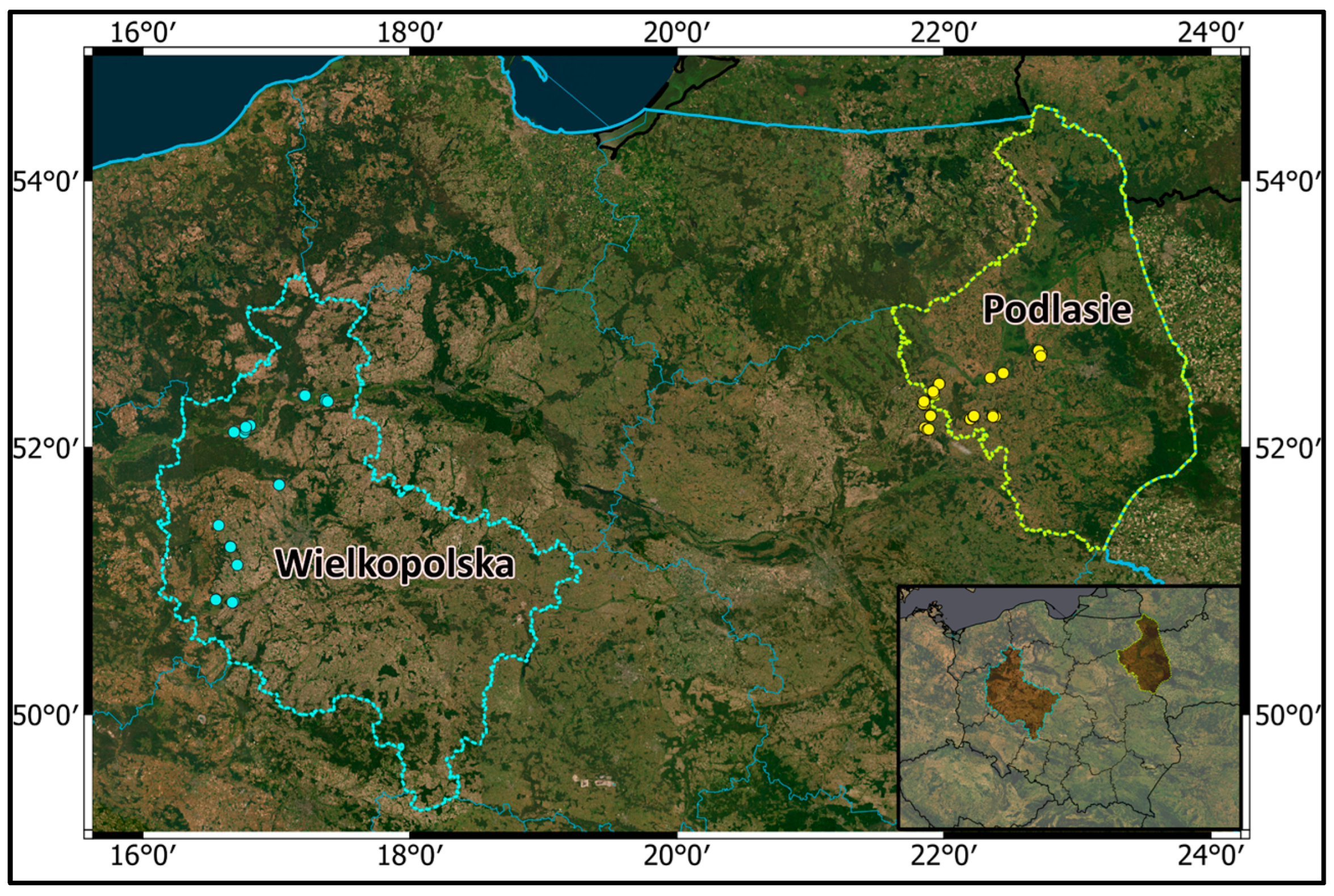
The study was conducted in a total of 46 areas in the north-eastern Podlasie region and the central-western Wielkopolska region of Poland (Figure 1). Podlasie is situated in the temperate transition climate zone and is characterized by pronounced continental influences, making it one of the coldest regions in Poland [15]. Podlasie region is an area where traditional and integrated farming systems are extensively practiced. The agricultural tradition in this region dates back to the early 15th century, and it has a long-standing agricultural heritage. It is considered one of the most developed and profitable agricultural areas in Poland [16]. Wielkopolska is distinguished by a warm, humid continental climate, characterized by moderate seasons. This region exhibits a climate structure marked by temperate summers and cold winters [17]. The Wielkopolska region is characterized by both agricultural production diversity and the presence of the dairy industry [18]. Grasslands in temperate regions, including Poland and other parts of Europe, typically undergo three cutting sessions annually [15].
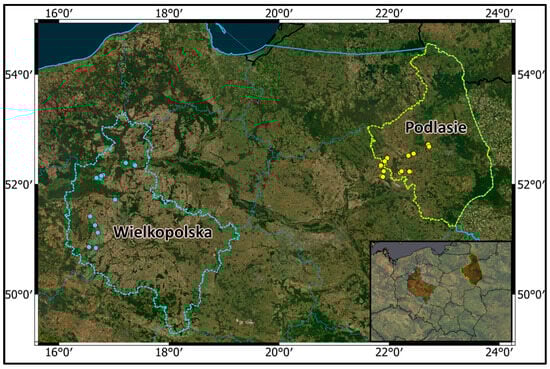
Figure 1.
Fields allocation map.
In situ measurements were taken during three different periods corresponding to the cuttings reported by farmers in the years 2020, 2021, and 2022. The first period was conducted at the end of April and in May. Measurements for the second period were carried out in June and July. The third period showed variations between July and September. LAI values and fresh biomass data were obtained during the measurements. LAI is commonly defined as half of the total green leaf area per unit of ground surface area [19]. It measures the leaf area within an ecosystem and is an essential factor in functions such as photosynthesis, respiration, and the interception of precipitation [20].
2.2. AquaCropP Model Overview
AquaCrop (Version: 7.0, Manufacturer Name: Food and Agriculture Organization of the United Nations (FAO), City: Rome, Country: Italy) [21] is a software system developed by the Land and Water Division of FAO [22]. The AquaCrop model forecasts crop yields and biomass in relation with water availability, considering rainfed conditions, as well as scenarios of deficit or full irrigation [23]. To simulate crop growth and yield, the AquaCrop model integrates soil physical and hydraulic processes, atmospheric factors (such as rainfall, temperature, evapotranspiration, ET, and carbon dioxide concentration), crop physiological characteristics, productivity parameters (including phenology, crop cover, root depth, biomass production, and harvestable yield), and field management practices (such as irrigation, fertilization, and agronomic techniques) [24]. In contrast to other models, it demonstrates higher efficacy in regions characterized by limited water availability, necessitates fewer parameters, and offers user-friendly features, increased accuracy, and reduced error probabilities [25]. Given that the Wielkopolska region is notably affected by the water deficit resulting from climate change, this model is particularly well-suited for the present study [5,26]. To simulate total biomass (B, kg), the model utilizes the cumulative actual transpiration (Tr, m3) over the growing season and normalized water productivity (WP, kgm−3) in its calculations) [27]:
The harvestable yield (Y) is calculated based on the total biomass (B, kg) and the harvest index (HI) as follows [27]:
2.3. Data Processing Methodology
The AquaCrop model is utilized to simulate crop growth and yield by incorporating atmospheric factors (such as rainfall, temperature, evaporation, transpiration, evapotranspiration, and carbon dioxide concentration), crop physiological characteristics, and productivity parameters (including phenology, crop canopy, and harvestable yield), along with soil properties. However, irrigation has not been applied to the grasslands in the study area, thus no data entry related to irrigation has been undertaken.
2.3.1. Required Input Data
AquaCrop is a model that simulates crop development and production based on inputs of climatic data, soil physical characteristics, crop attributes, and irrigation and field management information [28]. The climatic, crop, and soil characteristics data for the study areas were prepared following the model’s requirements.
2.3.2. Climatic Data
To generate climate files, the AquaCrop model requires daily measurements of rainfall, minimum and maximum air temperatures, reference crop evapotranspiration (ETo), and the average annual carbon dioxide concentration (CO2) [25]. The FAO Penman–Monteith method, as delineated in FAO Irrigation and Drainage Paper No. 56 [29], is utilized for calculating ETo, taking into consideration variables such as air temperature, humidity, wind speed, and solar radiation. The minimum air temperature (Tn) and maximum air temperature (Tx), dew point temperature (Tdew), wind speed at a height of x meters above the soil surface (u(x)), solar or shortwave radiation (Rs), and precipitation data have been acquired from the ERA5-Land Daily Aggregated dataset using the Google Earth Engine (GEE) platform. These data are utilized for the calculation of reference evapotranspiration (ETo) and for generating the climate file.
For the adjustment of crop transpiration and biomass water productivity, AquaCrop also requires the mean annual atmospheric CO2 concentration ([CO2]). The AquaCrop database comprises CO2 files, ‘MaunaLoa.CO2’, which encompasses observed mean annual [CO2] values spanning from 2000 to the present day [30].
2.3.3. Soil Profile Characteristics
Soil profile characteristics involve the physical attributes needed to model the retention and movement of water and salt within the soil, covering conditions at both the surface and the lower boundary where there is shallow groundwater [31]. These attributes include the volumetric water content at saturation (SAT), field capacity (FC), and permanent wilting point (PWP), as well as the hydraulic conductivity at soil saturation (Ksat), for each of the different soil horizons [30]. Soil data were collected from field measurements. Among the measured soil classes, the highest number of fields were found to belong to Eutric Histosol (15 fields) and Orthic Podzol (7 fields). Eutric Histosol, renowned for its high organic content, often characterizes wetland habitats and plays a vital role in water retention and nutrient cycling crucial for supporting diverse grassland vegetation. Conversely, Orthic Podzol, distinguished by its unique soil horizons and leaching processes, influences nutrient availability and water dynamics within grassland ecosystems. The identified soil types were matched with corresponding soil types in the AquaCrop database (Table S1). The attributes of these soil classifications in the model are contained in the default data. These values represent typical characteristics associated with each textural class and are based on extensive sampling and averaging (Table 1).

Table 1.
AquaCrop soil class characteristics.
2.3.4. Biomass Data
For grass types, dates have been identified based on measurements conducted in the field for the first, second, and third harvesting sessions. While the first harvesting typically falls between late April and late May, the second harvesting is often scheduled between mid-June and early July. As for the third harvesting, it usually occurs between early June and late September. The starting date for the first harvesting season in the model was estimated to be in August, considering the development of the grass. Subsequent mowing sessions were selected to follow each other at appropriate intervals.
AquaCrop Version 7.0 does not include a default file for grass. Therefore, a new crop file was created with the crop type set to ‘herbaceous forage crop.’ While compiling the crop file, the characteristics of perennial crops such as initial canopy cover, maximum canopy cover, and harvest index were inputted based on both in situ and satellite-derived LAI values. Self-thinning and fertility stress were not considered. The growth period was adjusted according to the dates obtained in the field. Within AquaCrop, simulations can be conducted using either calendar days or growing degree days [32]. In the Calendar Day Mode, the growth process is modeled based on calendar days, while in the Growing Degree Day Mode, it relies on a temperature-based approach. Calendar days were utilized to simulate grass development, taking into account the precise harvest date information provided by the farmer. In the perennial crop characteristics section of the crop file, the ‘1st season-sowing’ option was chosen for the first harvest, whereas for the second and third harvests, the ‘not first-regrowth’ option was selected.
For the adjustment of the crop development section, LAI values obtained from in situ measurements and Sentinel-2 data were utilized instead of canopy cover. The Sentinel-2 LAI data was provided by the Copernicus Land Monitoring Service (CLMS). LAI values available in the CLMS portfolio are updated daily and provided at a pan-European level, almost in real-time. The data covers the period from October 2016 to the present day and has a spatial resolution of 10 m × 10 m [33]. The green canopy cover (CC) represents the proportion of the soil surface covered by the canopy. It varies from zero at the time of sowing (0% of the soil surface covered by the canopy) to its maximum value at mid-season, reaching 1 when the canopy achieves full coverage (100% of the soil surface covered by the canopy) [30].
3. Results
3.1. Correlation Analysis of Biomass and Climatic Factors
The correlation matrices presented in Table 2 and Table 3 offer a comprehensive overview of the relationships between various variables related to biomass and climatic factors in the Podlasie and Wielkopolska regions, respectively. In the Podlasie region, consisting of 129 observations, significant associations are observed between in situ biomass and several climatic factors. Strong positive correlations are noted between in situ biomass and maximum temperature (Tmax), minimum temperature (Tmin), surface net solar radiation sum, and the date of observation, indicating that higher temperatures, increased solar radiation, and later dates, representing successive stages in the growing season, are generally associated with higher biomass levels. However, a weak negative correlation is found between dewpoint temperature and in situ biomass.
Table 2.
Correlation matrix of variables related to biomass and climatic factors for Podlasie region (N = 129, missing data were removed on a case-by-case basis).
Table 3.
Correlation matrix of variables related to biomass and climatic factors for Wielkopolska region (N = 112, missing data were removed on a case-by-case basis).
Conversely, in the Wielkopolska region, comprising 112 observations, the relationship between in situ biomass and climatic factors appears to differ. Here, in situ biomass shows weak negative correlations with several climatic factors.
Overall, the correlation matrices underscore the complex interplay between climatic factors and biomass levels in the two regions. While some similarities exist, such as the positive correlations among temperature-related variables, differences in the strength and direction of correlations highlight the unique environmental drivers shaping biomass dynamics in Podlasie and Wielkopolska regions.
3.2. Grassland Biomass Prediction in the Podlasie Region
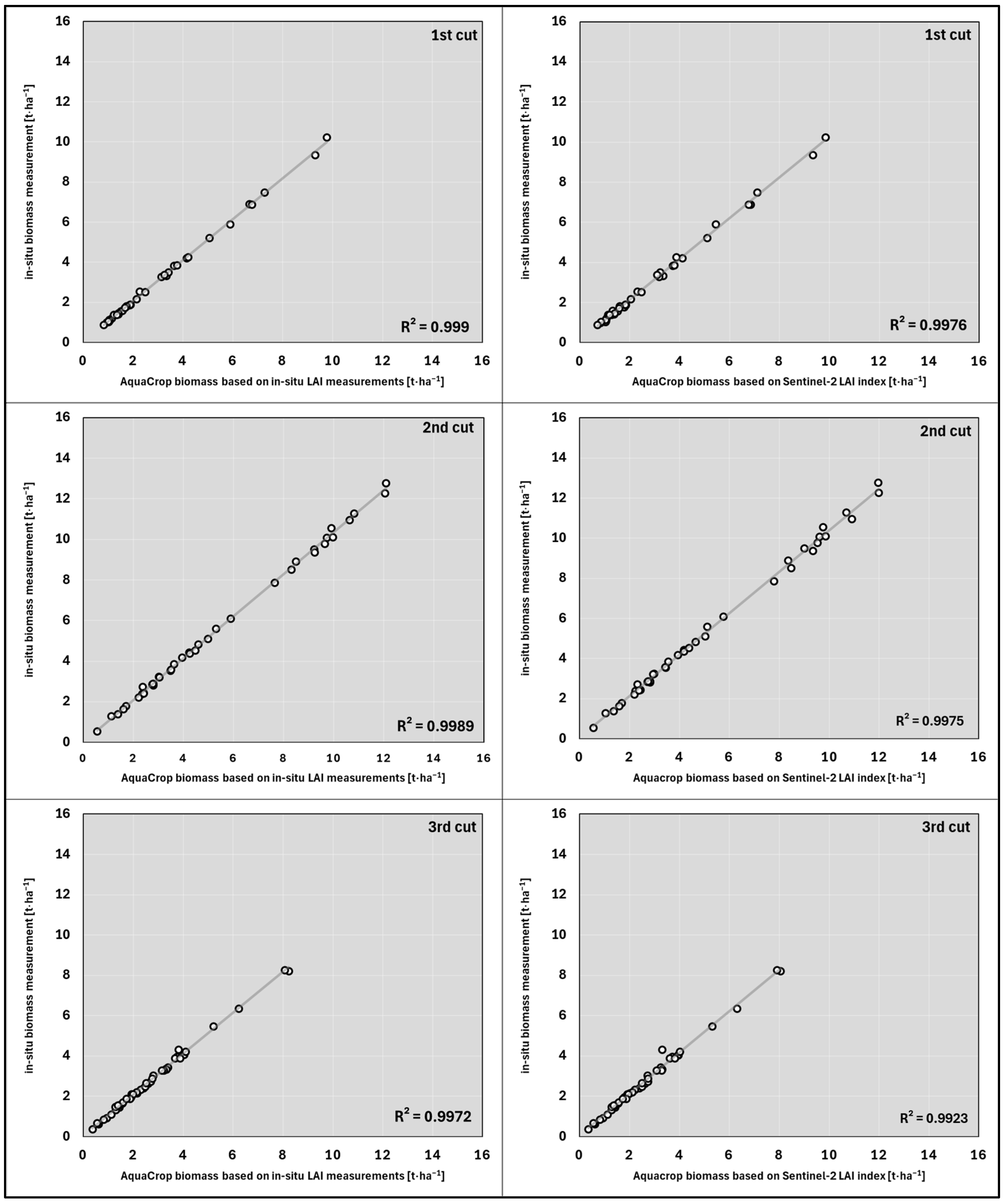
Figure 2 presents the results of biomass prediction using the AquaCrop model, where canopy cover is utilized as LAI in situ and LAI derived from Sentinel-2 data. The results are subdivided into three cuts, aggregated across three vegetation seasons. In the first column, comparisons depict the biomass prediction results based on LAI in situ against the actual biomass measured at the data collection points. Similarly, the second column provides comparisons between the same values, but with a canopy cover used as LAI from Sentinel-2. All AquaCrop model predictions demonstrate a coefficient of determination of approximately 0.99 when compared to actual biomass, indicating a very high level of model accuracy across various vegetation conditions and for different cuts.

Figure 2.
Prediction of biomass using AquaCrop model based on canopy cover as LAI in situ and LAI from Sentinel-2 data, aggregated across three vegetation seasons and three cuts in Podlasie region.
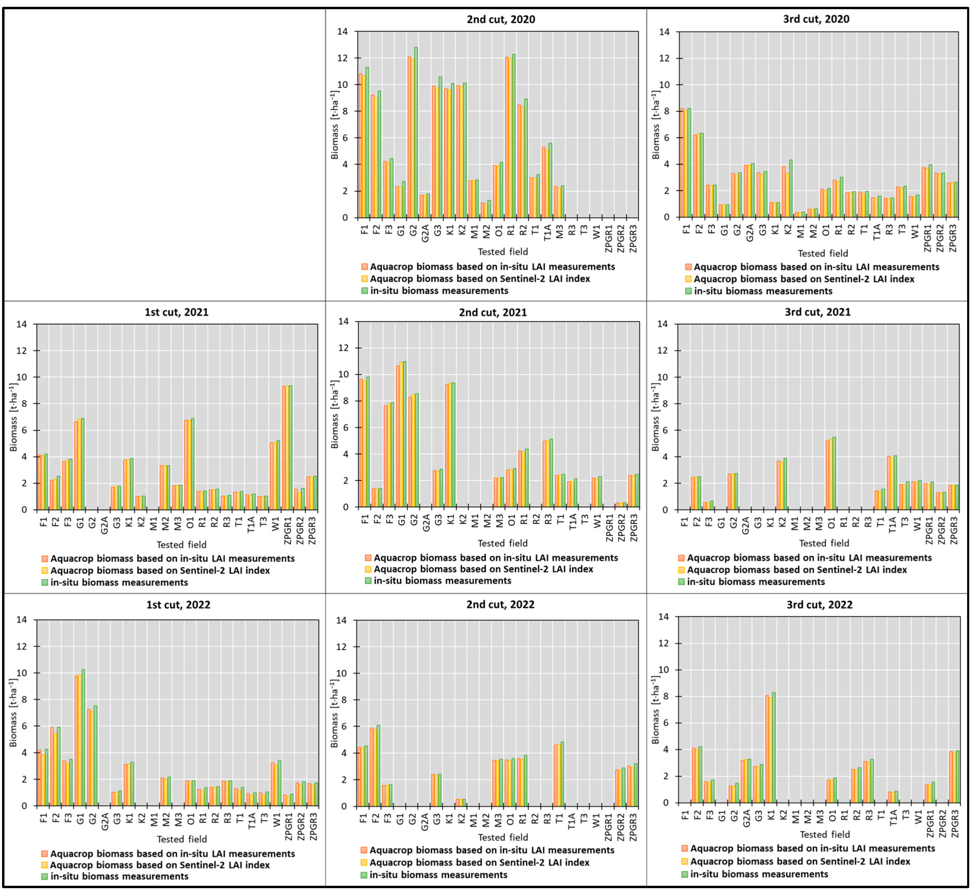
Figure 3 presents a comparative analysis of three datasets regarding biomass prediction across three vegetation seasons from 2020 to 2022. The rows of the figure correspond to individual years, while the columns represent different cuts. Each column chart comprises three bars: the first bar represents biomass prediction based on in situ LAI, the second bar represents biomass prediction based on LAI from Sentinel-2 data, and the third bar represents the actual biomass values measured in situ. The Y-axis of the chart denotes biomass values in tons per hectare. Upon examination of the charts for the years 2020 and 2021, it is evident that the second cut exhibited the highest biomass. However, in 2022, the first cut demonstrated the highest biomass among the same fields. Additionally, the third cut consistently yielded lower yields across all three vegetation seasons. In cases where there was a lack of in situ biomass data for specific fields, the corresponding fields on the charts remained empty.
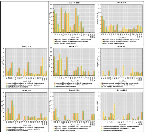
Figure 3.
Comparison of biomass prediction using in situ LAI, LAI from Sentinel-2, and actual biomass across three vegetation seasons and three cuts from 2020 to 2022 in Podlasie region.
3.3. Grassland Biomass Prediction in the Wielkopolska Region
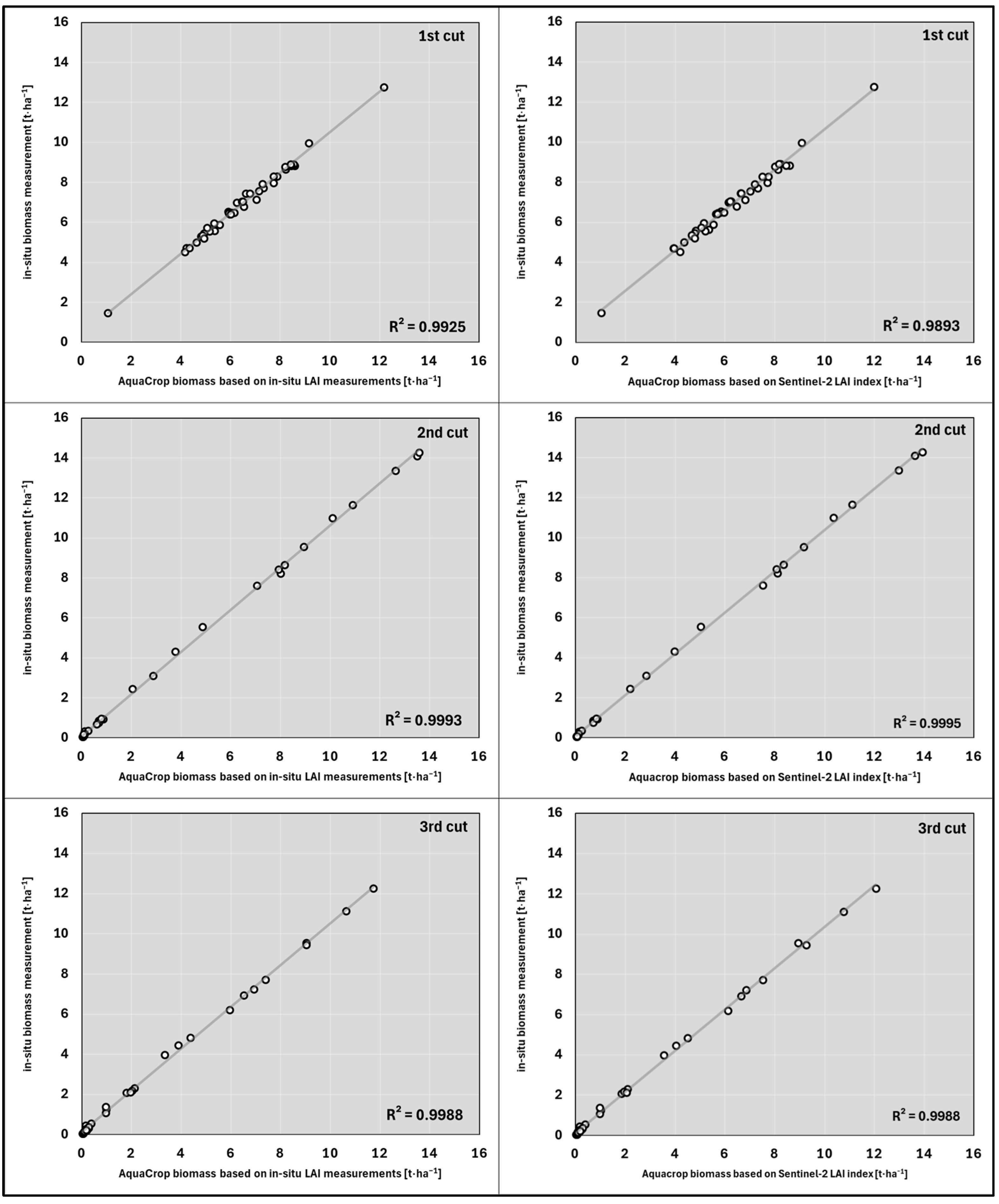
Figure 4 illustrates the prediction of biomass utilizing the AquaCrop model, where canopy cover serves as LAI in situ and LAI derived from Sentinel-2. The analysis is aggregated across three vegetation seasons and three cuts within the Wielkopolska region. Remarkably, the coefficient of determination (R2) for both LAI in situ and LAI from Sentinel-2 data ranges from 0.99 to 1.0 across all cuts and vegetation seasons. These high R2 values indicate an exceptional agreement between the predicted biomass and the actual biomass measured in situ. This suggests that the AquaCrop model, when utilizing canopy cover as LAI input, accurately predicts biomass levels across different cutting periods and vegetation seasons within the Wielkopolska region.

Figure 4.
Prediction of biomass using AquaCrop model based on Canopy Cover as LAI in situ and LAI from Sentinel-2 data, aggregated across three vegetation seasons and three cuts in Wielkopolska region.
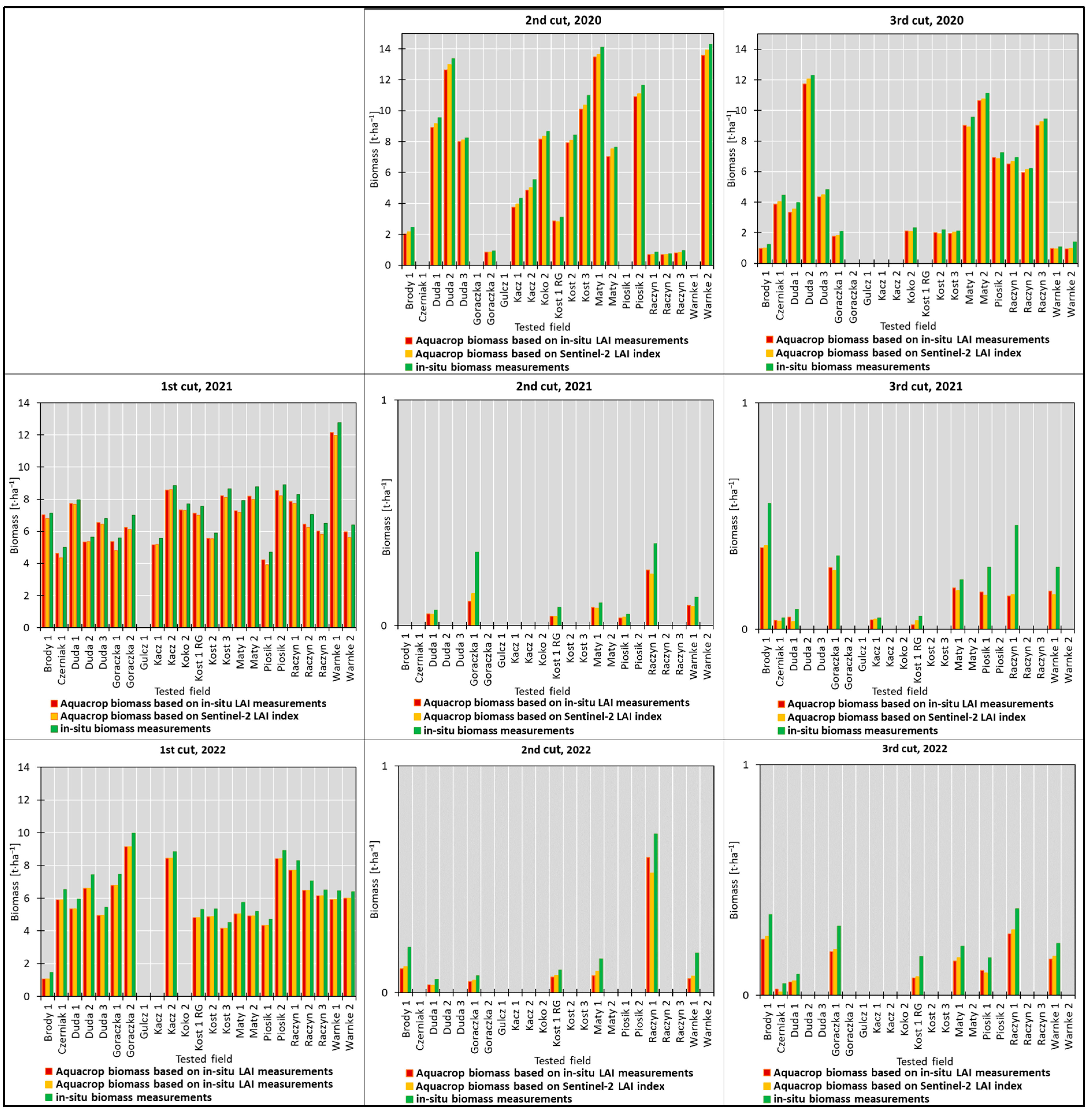
Figure 5 presents a comprehensive comparison of biomass prediction using in situ LAI, LAI from Sentinel-2, and actual biomass across three vegetation seasons and three cuts from 2020 to 2022 in the Wielkopolska region. The figure comprises eight comparative column charts, with years ranging from 2020 to 2022 arranged in rows and cuts in columns. Notably, there were no field studies conducted in 2020 for the first cut. The results exhibit significant variations compared to those observed in the Podlasie region.
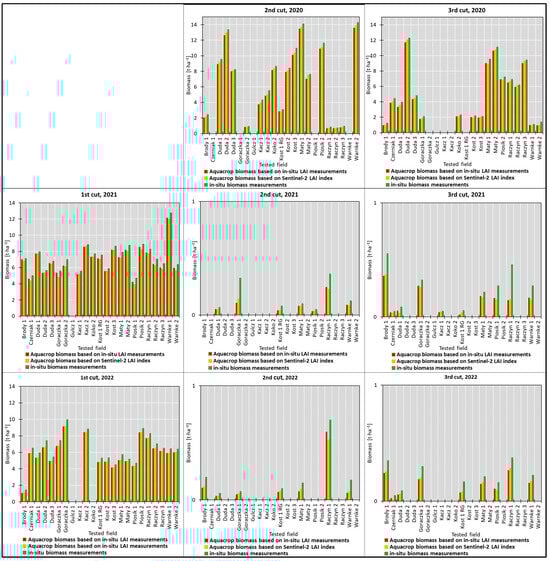
Figure 5.
Comparison of biomass prediction using in situ LAI, LAI from Sentinel-2, and actual biomass across three vegetation seasons and three cuts from 2020 to 2022 in Wielkopolska region.
In contrast to the Podlasie region, the first cut in the years 2021 and 2022 is characterized by relatively high biomass yields across all examined fields. However, the second and third cuts in the year 2020 significantly outweighed those in 2021 and 2022 in terms of biomass yield.
These findings suggest distinct patterns in biomass production across different cutting periods and vegetation seasons within the Wielkopolska region. Such variations underscore the importance of regional factors in influencing biomass dynamics and highlight the need for tailored agricultural management strategies to optimize biomass production in the region.
3.4. Comparative Evaluation of AquaCrop Model for Grass Biomass Prediction in Two Tested Regions
Figure 6 presents a comparison between LAI in situ measurements obtained from points tested in the Podlasie and Wielkopolska regions and Sentinel-2 CLMS data. The analysis covers vegetation periods characterized by three cuts. In the first cut, the determination coefficient (R2) between LAI obtained from Sentinel-2 in the Wielkopolska region and LAI measured in situ is impressively high, at 0.93. This indicates a strong alignment between the datasets. Data points in Wielkopolska are more densely clustered, whereas in Podlasie, they are more widely distributed. The regression line in Wielkopolska appears steeper than the one in Podlasie, indicating a stronger relationship between the Sentinel-2 LAI index and the in situ measured LAI in Wielkopolska.
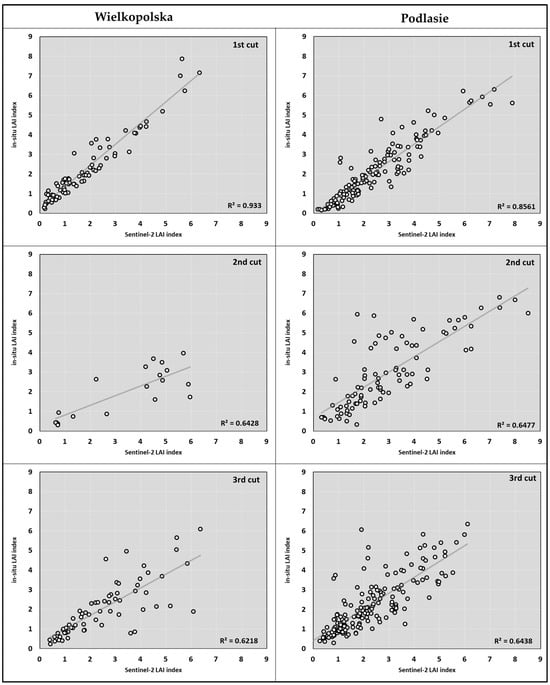
Figure 6.
Comparison of LAI index measured in situ and from Sentinel-2 CLMS for tested points in Podlasie region, aggregated across three vegetation seasons and three cuts.
In the second cut, the R2 value decreases to 0.64. When the regions are examined, the data points in the Wielkopolska region appear to be more scattered compared to those in the Podlasie region. This implies that the data points in the Wielkopolska region deviate more from the regression line. The regression model fits slightly less well in Wielkopolska compared to Podlasie.
For the third cut, a similar trend is observed with an R2 value of 0.62. While data points in Wielkopolska are more widely distributed, those in Podlasie exhibit a denser distribution. These findings reflect a consistent trend in R2 values across the second and third cuts. This suggests the presence of a consistent model in vegetation development.
These results underscore the importance of regional factors in influencing biomass dynamics and highlight the need for tailored agricultural management strategies to optimize biomass production in the region.
4. Discussion
Grasslands, while providing the foundation for ecosystem services by maintaining the balance of natural life, also significantly contribute to global food security by enhancing agricultural productivity. The areas of research in Poland are focused on harboring productive grasslands, thereby providing essential ecosystem services. However, increasingly prevalent climate change worldwide deeply affects grassland farming in these regions. Efforts are required to minimize these effects and enhance the resilience of grasslands. In our study, we conducted simulations to estimate biomass by simulating the growth of plants in grassland areas. Through these simulations, we aimed to monitor crop performance and take preventive measures against environmental impacts while enhancing efficiency in management. By utilizing both on-site measurements and remote sensing data in our research, we aimed to enable more effective and precise utilization of resources by evaluating plant growth strength and identifying changes in productivity.
In determining the use of satellite data in a study, the most critical factor is aligning the choice with the purpose and scope of the research. For instance, selecting satellite products suitable for the study’s objectives is paramount. Variables like the leaf area index (LAI) can effectively monitor plant growth, while SMAP satellite data may be preferable for measuring soil moisture levels. Additionally, prioritizing data with resolutions appropriate for the scale of the study is essential. The highest resolution might not always be necessary; different issues may demand varying resolution levels, spectral bands, and processing methods. It is crucial to verify the model’s universality concerning data availability, not only locally but also globally. If lower-resolution data fail to yield the expected results, then opting for higher-resolution data becomes necessary. In the conducted study, the results demonstrated the adequacy of incorporating data with different spatial resolutions into the model, producing satisfactory outcomes. Furthermore, temporal accessibility and financial feasibility are crucial considerations. Identifying suitable data for the required timeframe of the study and ensuring that the cost remains within acceptable levels are integral parts of the research process.
It has been observed that there is limited research on herbaceous forage crops using the AquaCrop model. While the AquaCrop model primarily focuses on annual crops, the modeling of specialized crops, such as perennial forage crops, has lagged behind [34]. This situation may be one reason why AquaCrop has less presence in the literature compared to other crop types. However, studies conducted on herbaceous forage crops using AquaCrop have yielded positive results.
One study [35] conducted between 2002 and 2006 in Stitar (Serbia) and Cukurova (Turkey), applied the AquaCrop model to evaluate the impact of different climatic conditions on Italian ryegrass crop density, biomass, and seed yields, and showed very good results. The biomass simulation was very good for Cukurova R2 = 0.97, but comparatively lower for Stitar R2 = 0.72. Under mild winter climate conditions, the AquaCrop model demonstrated greater reliability in predicting Italian ryegrass biomass.
In Raes et al.’s study (2023) [36], the objective was to simulate alfalfa yield by adapting AquaCrop’s 7th version to model perennial forage crops. Alfalfa (Medicago sativa L.) is a highly valued forage crop worldwide due to its perennial nature, nutritional richness, and deep root system, which enables it to access water and nutrients from the subsoil. Data collected from Louvain-La-Neuve (Belgium), Isparta (Turkey), and Ottawa (Canada) between 2013 and 2017 were utilized for the model’s evaluation. The assessment of cumulative aboveground biomass simulated during the growth cycle was highly satisfactory (R2 = 0.97; nRMSE = 11%; Nash–Sutcliffe model EF = 0.97).
The objective of the study conducted by Terán-Chaves et al. [37] in 2022 was to calibrate and validate the AquaCrop model for perennial ryegrass in the high tropics of Colombia (South America) over two consecutive seasons, spanning from 2008 to 2010. The experiments conducted during this period in perennial ryegrass meadows showed favorable statistical indicators, with R2 = 0.95 and RMSE = 2.63 t · ha−1.
Divergent viewpoints have been expressed regarding the necessity of irrigation for Miscanthus, particularly in areas with restricted water availability. Crop growth modeling can provide valuable insights to address such questions. Stričević et al. (2015) [38] utilized the FAO AquaCrop water-driven model to simulate Miscanthus biomass under various water supply conditions. Additionally, it is known that Miscanthus is found in the northeastern regions of Poland, where research has been conducted [39]. The research presents the findings from six years of experiments (2008–2013) conducted with Miscanthus at two locations in Serbia: Zemun and Ralja. The average RMSE was 2.89 , with deviations at the test site observed to be smaller in all years except the first. The coefficient of determination, R2, was determined to be 0.95. These results highlight a high level of agreement between the simulated and actual data.
Terán-Chaves et al. (2023), in their study [11], focused on assessing the capability of the AquaCrop-FAO model to predict the biomass (B) of Guinea grass (Megathyrsus maximus cv. Agrosavia sabanera) for the first time in the dry Caribbean region of Colombia, South America. The performance evaluation relied on field data gathered over the 2020/21 and 2021/22 growing seasons. The findings presented in this research offer an initial step towards tailoring the AquaCrop model for tropical pastures and other perennial herbaceous forage crops (PHFC). The cumulative biomass simulations yielded notably high accuracy, with R2 = 1.0 and RMSE = 5.13 .
Podlasie is located in a cold climatic zone with pronounced continental influences, whereas Wielkopolska enjoys a milder and more humid climate. These climatic differences have significant effects on plant growth and biomass production. Additionally, variations in soil properties can also influence biomass outcomes in both regions. Podlasie and Wielkopolska exhibit differences in soil types, nutrient content, and water retention capacities. These factors can impact the performance of the AquaCrop model, as the model takes into account climate and soil characteristics when calculating biomass production. Therefore, the variability in biomass predictions between Podlasie and Wielkopolska can be attributed to these climatic and soil properties.
The comparisons conducted within the literature indicate that our study demonstrates consistency with the results obtained by other researchers. The high consistency observed between the LAI values obtained from field measurements and those from Sentinel-2 satellite data is considered the primary reason for the high quality of results produced by the model and the strength of the statistical values. Understanding the key environmental components of grassland ecosystems enables accurate estimation of biomass not only in the eastern and western regions of Poland but also, as indicated by the literature, the AquaCrop model proves to be an effective tool for biomass prediction in various countries worldwide, beyond Europe.
5. Conclusions
The study underscores AquaCrop’s effectiveness in simulating biomass production for perennial herbaceous forage crops, offering a robust tool for bolstering agricultural sustainability and efficiency. By integrating both field measurements and satellite data, the model emerges as a valuable asset in decision-making processes, enabling a comprehensive understanding of the myriad factors influencing agricultural production. Furthermore, it illuminates the pivotal role of satellite data in refining agricultural models and enhancing their predictive capabilities.
However, it is essential to acknowledge certain limitations inherent in this study. While AquaCrop demonstrates proficiency in biomass prediction, its reliance on a singular simulation model may introduce biases and uncertainties. Moreover, the study’s focus on specific regions in Poland may constrain the generalizability of findings to broader geographic contexts, necessitating caution in extrapolating results to other regions.
Additionally, factors such as variability in soil conditions, land management practices, and local climate variations may impact the accuracy of biomass predictions, highlighting the need for further research to address these complexities.
Despite these limitations, the study underscores the importance of utilizing models like AquaCrop in broader agricultural studies, particularly in the face of significant challenges such as climate change.
Supplementary Materials
The following supporting information can be downloaded at: https://www.mdpi.com/article/10.3390/agriculture14060837/s1, AquaCrop soil characteristics corresponding to the measured soil classes are available in the supporting document. Table S1: AquaCrop soil class characteristics.
Author Contributions
Conceptualization, E.P.-C. and K.D.-Z.; methodology, E.P.-C., C.N.O. and K.D.-Z.; software, E.P.-C., C.N.O.; validation, E.P.-C., C.N.O.; formal analysis, E.P.-C., C.N.O.; investigation, E.P.-C. and K.D.-Z.; resources, E.P.-C. and K.W.; data curation, E.P.-C. and K.W.; writing—original draft preparation, E.P.-C., C.N.O.; writing—review and editing, E.P.-C.; visualization, E.P.-C.; supervision, E.P.-C. and K.D.-Z.; project administration, K.D.-Z.; funding acquisition, K.D.-Z. All authors have read and agreed to the published version of the manuscript.
Funding
This research was funded by The National Centre for Research and Development within the program “POLNOR 2019 call” under project number NOR/POLNOR/GrasSAT/0031/2019: “Tools for information to farmers on grasslands yields under stressed conditions to support management practices”(2020–2023).
Institutional Review Board Statement
Not applicable.
Data Availability Statement
The data supporting the reported results of this study are available upon request.
Acknowledgments
We extend our sincere gratitude to Professor Piotr Goliński and his dedicated team at Poznań University of Life Sciences, Department of Grassland and Natural Landscape Sciences, for their invaluable collaboration and guidance throughout the research process. We would also like to acknowledge the team at the Remote Sensing Center of the Institute of Geodesy and Cartography for conducting the field measurement campaigns in the years 2020–2022 and for providing the necessary database preparation.
Conflicts of Interest
The authors declare no conflicts of interest. The funders had no role in the design of the study, in the collection, analyses, or interpretation of data, in the writing of the manuscript; or in the decision to publish the results.
References
- Naicker, R.; Mutanga, O.; Peerbhay, K.; Odebiri, O. Estimating High-Density Aboveground Biomass within a Complex Tropical Grassland Using Worldview-3 Imagery. Environ. Monit. Assess. 2024, 196, 370. [Google Scholar] [CrossRef] [PubMed]
- Bazzo, C.O.G.; Kamali, B.; Hütt, C.; Bareth, G.; Gaiser, T. A Review of Estimation Methods for Aboveground Biomass in Grasslands Using UAV. Remote Sens. 2023, 15, 639. [Google Scholar] [CrossRef]
- Chen, P.; Wang, S.; Liu, Y.; Wang, Y.; Song, J.; Tang, Q.; Yao, Y.; Wang, Y.; Wu, X.; Wei, F. Spatio-temporal Dynamics of Aboveground Biomass in China’s Oasis Grasslands between 1989 and 2021. Earths Future 2024, 12, e2023EF003944. [Google Scholar] [CrossRef]
- GUS Agriculture in 2022. Available online: https://stat.gov.pl/en/topics/agriculture-forestry/agriculture/agriculture-in-2022,4,19.html (accessed on 16 April 2024).
- Gabryszuk, M.; Barszczewski, J.; Wróbel, B. Characteristics of Grasslands and Their Use in Poland. J. Water Land Dev. 2021, 243–249. [Google Scholar] [CrossRef]
- Adeboye, O.B.; Schultz, B.; Adeboye, A.P.; Adekalu, K.O.; Osunbitan, J.A. Application of the AquaCrop Model in Decision Support for Optimization of Nitrogen Fertilizer and Water Productivity of Soybeans. Inf. Process. Agric. 2021, 8, 419–436. [Google Scholar] [CrossRef]
- Panek, E.; Gozdowski, D.; Stępień, M.; Samborski, S.; Ruciński, D.; Buszke, B. Within-Field Relationships between Satellite-Derived Vegetation Indices, Grain Yield and Spike Number of Winter Wheat and Triticale. Agronomy 2020, 10, 1842. [Google Scholar] [CrossRef]
- Dabrowska-Zielinska, K.; Goliński, P.; Jørgensen, M.; Mølmann, J.; Taff, G.; Twardy, S.; Budzynska, M.; Czerwiński, M.; Kopacz, M.; Kurnicki, R.; et al. Importance of Grassland Monitoring in European Perspective of Climate Change—FINEGRASS Project. Geoinf. Issues 2016, 8, 55–71. [Google Scholar] [CrossRef]
- Panek, E.; Gozdowski, D. Relationship between MODIS Derived NDVI and Yield of Cereals for Selected European Countries. Agronomy 2021, 11, 340. [Google Scholar] [CrossRef]
- Gozdowski, D.; Stępień, M.; Panek, E.; Varghese, J.; Bodecka, E.; Rozbicki, J.; Samborski, S. Comparison of Winter Wheat NDVI Data Derived from Landsat 8 and Active Optical Sensor at Field Scale. Remote Sens. Appl. Soc. Environ. 2020, 20, 100409. [Google Scholar] [CrossRef]
- Terán-Chaves, C.A.; Mojica-Rodríguez, J.E.; Vega-Amante, A.; Polo-Murcia, S.M. Simulation of Crop Productivity for Guinea Grass (Megathyrsus Maximus) Using AquaCrop under Different Water Regimes. Water 2023, 15, 863. [Google Scholar] [CrossRef]
- Raes, D.; Steduto, P.; Hsiao, T.C.; Fereres, E. AquaCrop—The FAO Crop Model to Simulate Yield Response to Water: II. Main Algorithms and Software Description. Agron. J. 2009, 101, 438–447. [Google Scholar] [CrossRef]
- Vanuytrecht, E.; Raes, D.; Steduto, P.; Hsiao, T.C.; Fereres, E.; Heng, L.K.; Garcia Vila, M.; Mejias Moreno, P. AquaCrop: FAO’s Crop Water Productivity and Yield Response Model. Environ. Model. Softw. 2014, 62, 351–360. [Google Scholar] [CrossRef]
- Lombardo, S.; Mauromicale, G. Herbaceous Field Crops’ Cultivation. Agronomy 2021, 11, 742. [Google Scholar] [CrossRef]
- GUS Ochrona Środowiska i Leśnictwo w Województwie podlaskim w 2022 r. Available online: https://bialystok.stat.gov.pl/publikacje-i-foldery/ochrona-srodowiska/ochrona-srodowiska-i-lesnictwo-w-wojewodztwie-podlaskim-w-2022-r-,3,14.html (accessed on 16 April 2024).
- Castel, J.M.; Madry, W.; Gozdowski, D.; Roszkowska-Madra, B.; Dabrowski, M.; Lupa, W.; Mena, Y. Family Dairy Farms in the Podlasie Province, Poland: Farm Typology According to Farming System. Span. J. Agric. Res. 2010, 8, 946. [Google Scholar] [CrossRef]
- Goliński, P.; Czerwiński, M.; Jørgensen, M.; Mølmann, J.A.B.; Golińska, B.; Taff, G. Relationship between Climate Trends and Grassland Yield across Contrasting European Locations. Open Life Sci. 2018, 13, 589–598. [Google Scholar] [CrossRef] [PubMed]
- Bieńkowski, J.F.; Dąbrowicz, R.; Holka, M.; Jankowiak, J. Carbon Footprint of Rapeseed in Conventional Farming: Case Study of Large-Sized Farms in Wielkopolska Region (Poland). Asian J. Appl. Sci. Eng. 2014, 4, 191–200. [Google Scholar]
- Wang, Y.; Fang, H. Estimation of LAI with the LiDAR Technology: A Review. Remote Sens. 2020, 12, 3457. [Google Scholar] [CrossRef]
- Fang, H.; Baret, F.; Plummer, S.; Schaepman-Strub, G. An Overview of Global Leaf Area Index (LAI): Methods, Products, Validation, and Applications. Rev. Geophys. 2019, 57, 739–799. [Google Scholar] [CrossRef]
- AquaCrop|Land & Water|Food and Agriculture Organization of the United Nations|Land & Water|Food and Agriculture Organization of the United Nations. Available online: https://www.fao.org/land-water/databases-and-software/aquacrop/en/ (accessed on 10 April 2024).
- Er-Raki, S.; Bouras, E.; Rodriguez, J.C.; Watts, C.J.; Lizarraga-Celaya, C.; Chehbouni, A. Parameterization of the AquaCrop Model for Simulating Table Grapes Growth and Water Productivity in an Arid Region of Mexico. Agric. Water Manag. 2021, 245, 106585. [Google Scholar] [CrossRef]
- Mohamed Sallah, A.-H.; Tychon, B.; Piccard, I.; Gobin, A.; Van Hoolst, R.; Djaby, B.; Wellens, J. Batch-Processing of AquaCrop Plug-in for Rainfed Maize Using Satellite Derived Fractional Vegetation Cover Data. Agric. Water Manag. 2019, 217, 346–355. [Google Scholar] [CrossRef]
- Maniruzzaman, M.; Talukder, M.S.U.; Khan, M.H.; Biswas, J.C.; Nemes, A. Validation of the AquaCrop Model for Irrigated Rice Production under Varied Water Regimes in Bangladesh. Agric. Water Manag. 2015, 159, 331–340. [Google Scholar] [CrossRef]
- Umesh, B.; Reddy, K.S.; Polisgowdar, B.S.; Maruthi, V.; Satishkumar, U.; Ayyanagoudar, M.S.; Rao, S.; Veeresh, H. Assessment of Climate Change Impact on Maize (Zea Mays L.) through Aquacrop Model in Semi-Arid Alfisol of Southern Telangana. Agric. Water Manag. 2022, 274, 107950. [Google Scholar] [CrossRef]
- Kubiak-Wójcicka, K.; Machula, S. Influence of Climate Changes on the State of Water Resources in Poland and Their Usage. Geosciences 2020, 10, 312. [Google Scholar] [CrossRef]
- Mbangiwa, N.C.; Savage, M.J.; Mabhaudhi, T. Modelling and Measurement of Water Productivity and Total Evaporation in a Dryland Soybean Crop. Agric. For. Meteorol. 2019, 266–267, 65–72. [Google Scholar] [CrossRef]
- Zhang, T.; Zuo, Q.; Ma, N.; Shi, J.; Fan, Y.; Wu, X.; Wang, L.; Xue, X.; Ben-Gal, A. Optimizing Relative Root-Zone Water Depletion Thresholds to Maximize Yield and Water Productivity of Winter Wheat Using AquaCrop. Agric. Water Manag. 2023, 286, 108391. [Google Scholar] [CrossRef]
- Cheng, M.; Wang, H.; Fan, J.; Xiang, Y.; Liu, X.; Liao, Z.; Abdelghany, A.E.; Zhang, F.; Li, Z. Evaluation of AquaCrop Model for Greenhouse Cherry Tomato with Plastic Film Mulch under Various Water and Nitrogen Supplies. Agric. Water Manag. 2022, 274, 107949. [Google Scholar] [CrossRef]
- Raes, D. AquaCrop Training Handbook I. Understanding AquaCrop August 2023; Food and Agriculture Organization of the United Nations: Rome, Italy, 2023. [Google Scholar]
- Raes, D.; Steduto, P.; Hsiao, T.C.; Fereres, E. Reference Manual for AquaCrop Version 7.1—Chapter 2; Food and Agriculture Organization of the United Nations: Rome, Italy, 2023. [Google Scholar]
- Coudron, W.; Gobin, A.; Boeckaert, C.; De Cuypere, T.; Lootens, P.; Pollet, S.; Verheyen, K.; De Frenne, P.; De Swaef, T. Data Collection Design for Calibration of Crop Models Using Practical Identifiability Analysis. Comput. Electron. Agric. 2021, 190, 106457. [Google Scholar] [CrossRef]
- Leaf Area Index, CLMS. Available online: https://land.copernicus.eu/en/products/vegetation/high-resolution-leaf-area-index (accessed on 15 April 2024).
- Alavipanah, S.K.; Matinfar, H.R.; Emam, A.R.; Khodaei, K.; Bagheri, R.H.; Panah, Y. Criteria of Selecting Satellite Data for Studying Land Resources. Desert 2010, 15, 83–102. [Google Scholar]
- Stricevic, R.; Simic, A.; Kusvuran, A.; Cosic, M. Assessment of AquaCrop Model in the Simulation of Seed Yield and Biomass of Italian Ryegrass. Arch. Agron. Soil Sci. 2017, 63, 1301–1313. [Google Scholar] [CrossRef]
- Raes, D.; Fereres, E.; García Vila, M.; Curnel, Y.; Knoden, D.; Çelik, S.K.; Ucar, Y.; Türk, M.; Wellens, J. Simulation of Alfalfa Yield with AquaCrop. Agric. Water Manag. 2023, 284, 108341. [Google Scholar] [CrossRef]
- Terán-Chaves, C.A.; García-Prats, A.; Polo-Murcia, S.M. Calibration and Validation of the FAO AquaCrop Water Productivity Model for Perennial Ryegrass (Lolium Perenne L.). Water 2022, 14, 3933. [Google Scholar] [CrossRef]
- Stričević, R.; Dželetović, Z.; Djurović, N.; Cosić, M. Application of the AquaCrop Model to Simulate the Biomass of Miscanthus x Giganteus under Different Nutrient Supply Conditions. GCB Bioenergy 2015, 7, 1203–1210. [Google Scholar] [CrossRef]
- Dubis, B.; Jankowski, K.J.; Załuski, D.; Bórawski, P.; Szempliński, W. Biomass Production and Energy Balance of Miscanthus over a Period of 11 Years: A Case Study in a Large-scale Farm in Poland. GCB Bioenergy 2019, 11, 1187–1201. [Google Scholar] [CrossRef]

Disclaimer/Publisher’s Note: The statements, opinions and data contained in all publications are solely those of the individual author(s) and contributor(s) and not of MDPI and/or the editor(s). MDPI and/or the editor(s) disclaim responsibility for any injury to people or property resulting from any ideas, methods, instructions or products referred to in the content. |
© 2024 by the authors. Licensee MDPI, Basel, Switzerland. This article is an open access article distributed under the terms and conditions of the Creative Commons Attribution (CC BY) license (https://creativecommons.org/licenses/by/4.0/).