Research on the Temporal and Spatial Changes and Driving Forces of Rice Fields Based on the NDVI Difference Method

Abstract

Rice is a globally important food crop, and it is crucial to accurately and conveniently obtain information on rice fields, understand their spatial patterns, and grasp their dynamic changes to address food security challenges. In this study, Chongqing’s Yongchuan District was selected as the research area. By utilizing UAVs (Unmanned Aerial Vehicles) to collect multi-spectral remote sensing data during three seasons, the phenological characteristics of rice fields were analyzed using the NDVI (Normalized Difference Vegetation Index). Based on Sentinel data with a resolution of 10 m, the NDVI difference method was used to extract rice fields between 2019 and 2023. Furthermore, the reasons for changes in rice fields over the five years were also analyzed. First, a simulation model of the rice harvesting period was constructed using data from 32 sampling points through multiple regression analysis. Based on the model, the study area was classified into six categories, and the necessary data for each region were identified. Next, the NDVI values for the pre-harvest and post-harvest periods of rice fields, as well as the differences between them, were calculated for various regions. Additionally, every year, 35 samples of rice fields were chosen from high-resolution images provided by Google. The thresholds for extracting rice fields were determined by statistically analyzing the difference in NDVI values within the sample area. By utilizing these thresholds, rice fields corresponding to six harvesting regions were extracted separately. The rice fields extracted from different regions were merged to obtain the rice fields for the study area from 2019 to 2023, and the accuracy of the extraction results was verified. Then, based on five years of rice fields in the study area, we analyzed them from both temporal and spatial perspectives. In the temporal analysis, a transition matrix of rice field changes and the calculation of the rice fields’ dynamic degree were utilized to examine the temporal changes. The spatial changes were analyzed by incorporating DEM (Digital Elevation Model) data. Finally, a logistic regression model was employed to investigate the causes of both temporal and spatial changes in the rice fields. The study results indicated the following: (1) The simulation model of the rice harvesting period can quickly and accurately determine the best period of remote sensing images needed to extract rice fields. (2) The confusion matrix shows the effectiveness of the NDVI difference method in extracting rice fields. (3) The total area of rice fields in the study area did not change much each year, but there were still significant spatial adjustments. Over the five years, the spatial distribution of gained rice fields was relatively uniform, while the lost rice fields showed obvious regional differences. In combination with the analysis of altitude, it tended to grow in lower areas. (4) The logistic regression analysis revealed that gained rice fields tended to be found in regions with convenient irrigation, flat terrain, lower altitude, and proximity to residential areas. Conversely, lost rice fields were typically located in areas with inconvenient irrigation, long distance from residential areas, low population, and negative topography.

1. Introduction

Rice, as a globally significant food crop, holds a critical position in food production. Being the primary source of sustenance for nearly half of the world’s population, it exerts a substantial influence on global politics and economics [1]. According to United Nations projections, the global population is expected to reach nearly 10 billion by 2050 [2]. In the face of immense population pressures, the global food security situation is becoming increasingly critical and complex [3]. Therefore, the acquisition of rice field information, and understanding of the spatial pattern and dynamic changes of rice fields, are of great significance for estimating rice production, formulating relevant strategies, adjusting and optimizing spatial layout, and rationally allocating resources to address food security challenges [4].

Both domestic and international scholars have conducted extensive research on the dynamic changes in spatiotemporal patterns of rice fields, focusing on two main areas: the extraction of rice field information and the analysis of the drivers behind the dynamics of rice fields’ spatiotemporal changes [5,6]. The existing methods for extracting rice fields can be classified into two main categories: integrated extraction and individual extraction. Integrated extraction refers to directly extracting rice fields using land use data, but it becomes challenging due to variations in classification criteria. Even though it is possible to extract data through manual visual interpretation, the time and monetary costs are relatively high. Therefore, most data products rely on machine learning as the core approach for classification. However, these products primarily focus on cultivated land. Consequently, the latter method, which is individual extraction, needs to take into account the characteristics specific to rice fields. Rice is one of the world’s important crops, and as a special seasonal vegetation, a crop that has distinct phenological characteristics [7,8]. Therefore, some scholars have extracted rice field information by combining machine learning with rice fields’ phenological characteristics. Commonly used data sources include MODIS (Moderate Resolution Imaging Spectroradiometer), Landsat, and Sentinel-2, among which MODIS data have a high temporal resolution but moderate spatial resolution and are often used to obtain global- or national-scale rice information. Landsat and Sentinel-2, on the other hand, have a relatively high spatial resolution and medium temporal resolution. To obtain high temporal and spatial resolution data, MODIS data have been fused with Sentinel-2 data using the RASTFM (Robust Adaptive Spatial Temporal Fusion Model). To eliminate the noise in the fused time series Sentinel-2 NDVI data caused by cloud contamination and errors during prediction, the NDVI data have been smoothed using an S-G (Savitzky–Golay) filter, and the phenological parameters have been extracted from the filtered NDVI time series using a thresholding method. Finally, the Random Forest algorithm has been utilized to extract rice fields. However, the accuracy of the Sentinel-2 time series is compromised in this method, and there is also a reduction in accuracy due to the issue of mixed pixels [9]. In a separate study, by utilizing Landsat 8 data, the NDVI time series and the temporal profiles of LST (Land Surface Temperature) have been studied to distinguish rice fields. However, the use of Landsat 8 with a resolution of 30 m in this research leads to variations between the extracted rice fields results and the ground truth [10]. Rice NDVI time series curves have been established based on field surveys and Google Earth sample data. The DTW (Dynamic Time Warping) distance for each pixel’s rice NDVI time series was then calculated to extract the rice area using a threshold. This study employed the DTW method to assess the similarity or difference between the curves. However, the DTW distances were found to be smaller for standard NDVI curve shapes, which are less dynamic in rice field phenology, leading to some limitations in identification [11]. Differing from the aforementioned study, based on the unique characteristics of rice fields that have large differences in vegetation between the pre-harvest and post-harvest periods, the NDVI difference method has been used to extract rice fields using Sentinel-2 data. The extraction of rice fields only utilizes specific phenological periods and a few indicators. This approach accurately and quickly obtains information about rice fields with good results. However, due to the similar rice harvesting periods and limited variety of land cover types in the study area, it is not sufficient to demonstrate the generality of this method [12]. For the spatial-temporal changes and driving forces of rice fields, the evolution of crop spatial patterns is a complex process influenced by multiple factors rather than a single factor. These factors include natural factors, socio-economic factors, input factors, technological progress factors, as well as agricultural policy factors, among others [13,14,15]. In terms of research methods, various approaches are employed, such as principal component analysis, grey relational analysis, and canonical correlation analysis. However, the methods above primarily focus on quantitative research, making it difficult to analyze spatial heterogeneity. The influencing factors on the spatiotemporal pattern of soybean production in Sichuan Province from 2000 to 2020 have been explored using the parametric optimal geographic detector. However, this method has uncertainty in determining the positive and negative effects of the influencing factors, and further exploration is needed [16]. In contrast, there has been a study that has analyzed the driving factors of cultivated land conversion in the Yellow River Delta over the past 30 years using the logistic regression model [17]. This model can be used for regression analysis with a categorical dependent variable, where the independent variables can be either continuous or discrete. On the other hand, there are few studies currently that directly investigate changes in patches based on two or multiple time-period data. Moreover, most of these studies also employ the logistic regression model, which can effectively explore the causes and underlying mechanisms of the changes [18,19].

This article aims to use the NDVI difference method to analyze the spatiotemporal changes of rice fields in Yongchuan District, Chongqing. The logistic regression model examines the driving forces behind these changes and uncovers the factors contributing to the transformation of rice fields. The findings of this study serve as valuable references for decision-making in future agricultural production and land spatial planning.

2. Materials and Methodology

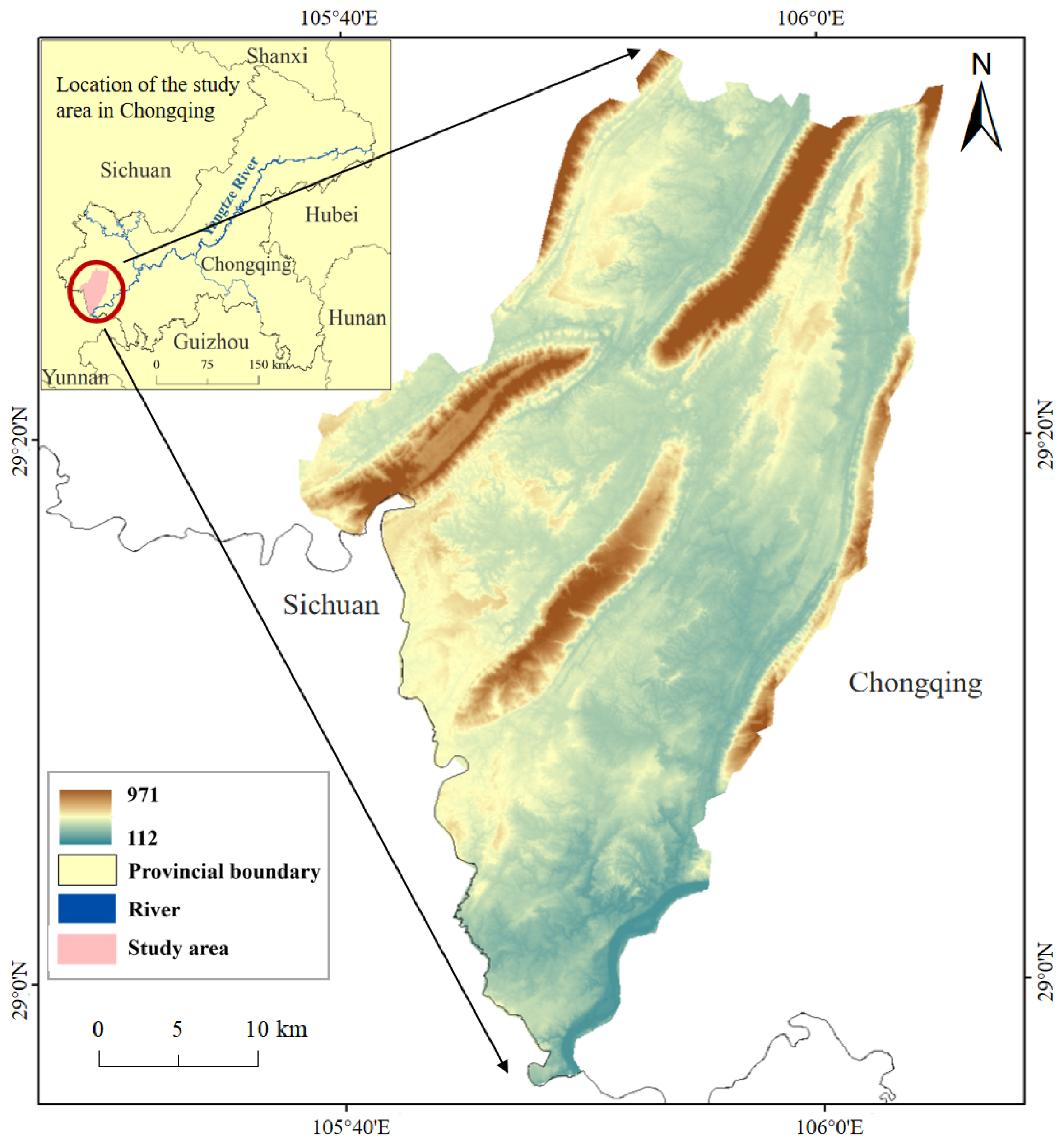
2.1. Study Area

The study area is located in Yongchuan District, Chongqing City. It is situated on the northern bank of the upper Yangtze River, in the western part of Chongqing (between 105°38′ to 106°5′ E and 29°45′ to 29°52′ N) (Figure 1). The total area is approximately 1.6 × 10⁵ hm². The terrain consists mainly of shallow hills with a flat topography. Four low mountain ranges run from northeast to southwest, with elevations ranging from 112 m to 971 m. The climate is classified as subtropical monsoon humid climate, with warm winters and hot summers, experiencing minimal frost and snow, with an average annual temperature of about 17.7 °C; short sunshine durations, with an average annual sunshine length of about 1298.5 h; and abundant precipitation, with an average annual rainfall of 1015 mm, but the spatial and temporal distribution is not uniform, and it is concentrated in summer, belonging to the area of cloudy and rainy [20,21]. According to the meteorological data, the main weather in Yongchuan District in the past year 2023 was rainy, cloudy, partly cloudy, and sunny, accounting for about 126 days, 91 days, 60 days, and 55 days, respectively. On the other hand, the study area is abundant in natural resources, with six rivers running across it from north to south. Moreover, it is one of the primary grain-producing areas in Chongqing and the region where rice matures relatively early. According to the statistical yearbook, in recent years, the rice cultivation area is around 4.0 × 10⁴ hm², with a production of approximately 3.4 × 10⁵ t. As a vital hub in the Chengdu–Chongqing dual-city economic circle and a strategic support point of the main urban area of Chongqing, it enjoys fast and convenient communication and transportation. Furthermore, the Chengdu–Chongqing Expressway and Chengdu–Chongqing Railway span from the east to the west [22].

2.2. Data Source and Pre-Processing

The data used in this study include Sentinel-2 data, multi-spectral remote sensing data, rice harvesting period data, and other data related to nature, social, and economic factors. First of all, Sentinel-2, which originates from the European Space Agency, consists of Sentinel-2A and Sentinel-2B. These satellites are equipped with the MSI (Multispectral Imager) sensor, which enables repetitive monitoring of the Earth’s land surface [23]. The sensor offers 13 spectral wavebands: B2, B3, B4, and B8, which have a resolution of 10 m; B5, B6, B7, B8A, B11, and B12 have a resolution of 20 m; and B1, B9, and B10 have a resolution of 60 m (

Table 1. Sentinel-2 band information table.

Sentinel-2 Bands	Central Wavelength (nm)		Spatial Resolution (m)
	Sentinel-2A	Sentinel-2B
B1- Coastal Aerosol	443.9	442.3	60
B2- Blue	496.6	492.1	10
B3- Green	560.0	559	10
B4- Red	664.5	665	10
B5- Vegetation Red Edge	703.9	703.8	20
B6- Vegetation Red Edge	740.2	739.1	20
B7- Vegetation Red Edge	782.5	779.7	20
B8- NIR	835.1	833	10
B8A- Narrow NIR	864.8	864	20
B9- Water Vapor	945.0	943.2	60
B10- SWIR-Cirrus	1373.5	1376.9	60
B11- SWIR	1613.7	1610.4	20
B12- SWIR	2202.4	2185.7	20

). As this study focused primarily on extracting rice fields using NDVI difference values from the pre-harvest and post-harvest periods, it predominantly utilized bands 4 and 8 [24]. Therefore, the NDVI data obtained had a resolution of 10 m. These data were used to extract rice field information from 2019 to 2023 in the study area for further analysis. The data pre-processing included radiometric calibration, atmospheric correction, resampling, and band fusion of the products. Secondly, the multi-spectral remote sensing data were acquired using DJI multi-spectral UAV for analyzing the phenological characteristics of rice fields in the study area. Furthermore, data on the rice harvesting period were used to construct the rice harvesting model, which was mainly obtained through data collection and on-site surveys. Finally, additional data related to natural, social, and economic factors were utilized to analyze the driving forces behind the spatiotemporal changes in rice fields. These data include digital elevation data, water systems, rural roads, settlements, population density, and relevant statistical yearbook data. The DEM data are sourced from the official NASA (National Aeronautics and Space Administration) website (https://search.asf.alaska.edu/ (accessed on 15 September 2023)), with a spatial resolution of 12.5 m. The water system data are obtained from OpenStreetMap. The rural road data are sourced from the third national land survey. The settlement data are obtained from the National Basic Geographic Information Center. The population density data are derived from LandScan and WorldPop datasets. The LandScan data have a resolution of 1 km and were developed by the ORNL (Oak Ridge National Laboratory) of the U.S. Department of Energy. The WorldPop data have a resolution of 100 m and were developed by the Department of Geography at the University of Florida and the Institute for New Pathogens Research. They can be downloaded from the website (www.worldpop.org). A major focus of WorldPop is improving the spatial demographic evidence base for low and middle-income countries, as well as collaborating with many national statistical offices and ministries of health around the world, providing training and support [25]. The relevant statistical yearbooks are sourced from official government websites.

2.3. Methodology

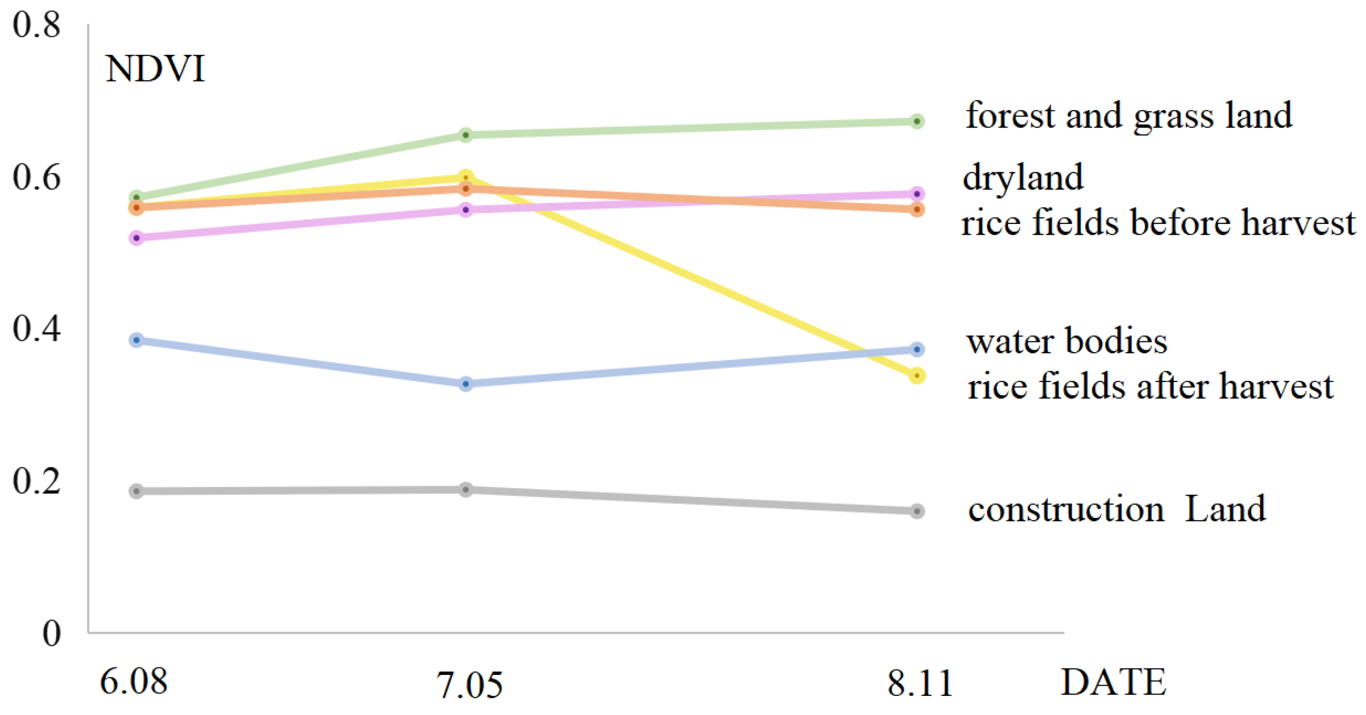
2.3.1. Analysis of Phenological Characteristics Based on NDVI Values in Rice Fields

NDVI serves as an effective indicator for monitoring vegetation dynamics, allowing for quantitative assessment of regional vegetation coverage and growth conditions [26,27]. To acquire the phenological characteristics of rice in the research area, sample areas were selected, and multi-spectral remote sensing data were collected using UAV on 8 June, 5 July, and 11 August 2023. The NDVI values were calculated based on Equation (1), where NIR represents the near-infrared band and R represents the red band.

$$\mathrm{NDVI}={\displaystyle \frac{\mathrm{NIR}-\mathrm{R}}{\mathrm{NIR}+\mathrm{R}}}$$

(1)

To compare various ground feature samples at different periods (Figure 2), Figure 2a illustrates the unmanned aerial vehicle remote sensing image, while Figure 2b represents the computed NDVI image. The colors, ranging from dark to light, indicate low to high NDVI values. According to Figure 2, it can be observed that there is relatively little overall change in the ground features and their corresponding NDVI values in the sample areas between 8 June and 5 July 2023. However, between 5 July and 11 August 2023, there is noticeable harvesting occurring in certain rice fields, accompanied by significant changes in their NDVI values. Therefore, for ease of analysis, the rice fields are highlighted through marking, with red marking indicating unharvested rice and yellow marking indicating harvested rice. Specifically, the rice fields that experienced harvesting show a significant decrease in NDVI values, while the NDVI values in the rice fields that are not harvested remain relatively stable. Additionally, there are no significant changes observed in other land classes.

To further analyze the trend of changes, the time-series NDVI curves (Figure 3) were constructed by randomly selecting samples of various ground features based on unmanned aerial remote sensing images and computed NDVI values. Based on Google imagery and field investigations, the main ground features observed in the study area included rice fields, dry land, water bodies, construction land, and forest and grassland. From the analysis of the trend and degree of change, it is found that the harvested rice fields experience a significant decrease in NDVI values during the period from 5 July to 11 August, with a difference of 0.26. However, the NDVI values of rice fields that are not harvested remain relatively stable. The reason for the higher NDVI values in rice fields before the harvest is their vigorous growth. However, after the harvest, the NDVI values significantly decrease. Moreover, there is relatively little change in the NDVI values of other ground features between the pre-harvest and post-harvest periods of rice fields. Consequently, this characteristic can be used to distinguish and identify rice fields.

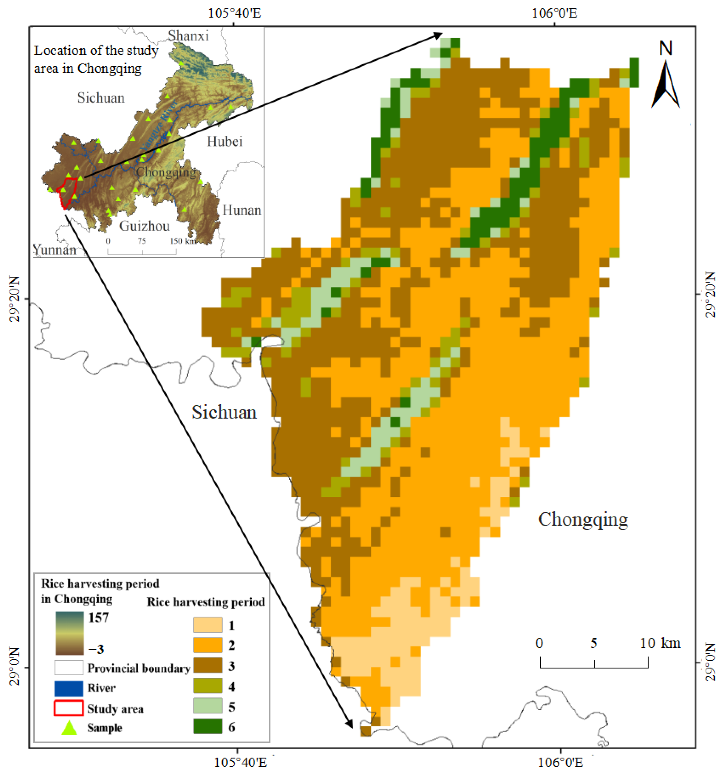
2.3.2. Spatial and Temporal Simulation of the Rice Harvesting Period

To extract rice fields using the difference in NDVI values between the pre-harvest and post-harvest periods of rice fields, it was crucial to determine the harvest period. Through data inquiry and field visits, it was discovered that the harvest period of rice fields in different regions was influenced by altitude and latitude [28]. Therefore, a rice harvest period model was constructed using these two indicators. The software used for data analysis was IBM SPSS Statistics 25, known for its in-depth analysis capabilities, ease of use, and comprehensive functions, making it widely applicable across various fields [29]. The rice harvesting period was a time range, but for the convenience of subsequent model construction, a single value representing the period between the pre-harvest and post-harvest stages of rice fields was temporarily used to represent the harvesting period. This study randomly selected 32 sample points and collected relevant information (

Table 2. Rice harvesting sample points information.

Sample point numbers	Elevation X1 (m)	Latitude X2 (°)	Rice Harvesting Period Y
1	275	29.33	7 (7 August 2023)
2	324	29.33	10 (10 August 2023)
3	260	29.61	10 (10 August 2023)
4	346	30.26	20 (20 August 2023)
5	274	29.19	8 (8 August 2023)
6	268	29.77	11 (11 August 2023)
7	400	29.55	17 (17 August 2023)
8	267	30.28	15 (15 August 2023)
9	457	29.89	15 (15 August 2023)
10	363	28.90	6 (6 August 2023)
11	546	28.82	16 (16 August 2023)
12	615	29.35	23 (23 August 2023)
13	705	29.13	31 (31 August 2023)
14	383	29.87	18 (18 August 2023)
15	414	30.32	24 (24 August 2023)
16	852	29.31	42 (11 September 2023)
17	317	29.90	15 (15 August 2023)
18	369	30.00	20 (20 August 2023)
19	422	30.70	25 (25 August 2023)
20	491	30.08	28 (28 August 2023)
21	165	31.14	10 (10 August 2023)
22	223	30.40	16 (16 August 2023)
23	812	28.89	30 (30 August 2023)
24	751	31.79	53 (22 September 2023)
25	1150	29.43	60 (29 September 2023)
26	370	30.89	27 (27 August 2023)
27	742	30.88	47 (16 September 2023)
28	284	29.36	10 (10 August 2023)
29	371	30.89	25 (25 August 2023)
30	690	31.33	46 (15 September 2023)
31	359	31.06	23 (23 August 2023)
32	317	30.67	26 (26 August 2023)

), with altitude and latitude as independent variables and harvesting period as the dependent variable. Partial correlation analysis was conducted using SPSS Statistics. Under the relevant assumptions, the rice harvest model was constructed using the multiple linear regression analysis tool in SPSS. Based on the analysis results, the overall explanatory power of the independent variables on the dependent variable reached 96%, indicating a good fit. Additionally, the fitted equation was statistically significant, with constants, latitude, and elevation all having significance levels of less than 0.001. Therefore, the regression model demonstrated significant effectiveness.

Due to the vast expanse of Chongqing City, accurately representing its continuity is challenging, despite the latitude being distributed continuously [30]. Consequently, Chongqing was divided into a grid of 1 km by 1 km cells, and the latitude value of each grid center was obtained. Then, based on the 12.5 m resolution DEM data, the average elevation values for each grid cell were calculated, and these values, along with the central latitude, were input into the model of the rice harvesting period. Using the raster calculator, the rice harvesting period values for each grid cell were calculated, thereby obtaining the simulated rice harvesting period values for the entire Chongqing area. Thus, the rice harvesting time in the study area was determined. The data were then reclassified into nine categories at equal time intervals of 5 days.

Finally, the Sentinel-2 data during the pre-harvest and post-harvest periods of rice fields in the study area were determined based on the simulated harvest period. The selected differential data needed to include the actual harvesting period in the region, ensuring the complete extraction of all rice fields in the area, while avoiding large time intervals that could result in interference from other factors. Apart from the time requirement, the data quality also needed to be ensured. Due to the cloudy and rainy conditions in the study area [31], it proved challenging to extract information about the entire rice fields using just two sets of data. Therefore, considering all factors, three sets of data were used as sources for each year.

Table 3. Data sources correspond to different regions during the harvesting periods in the study area.

Year	Data sources corresponding to different regions during the harvesting periods
2019	1, 2, 3	4, 5, 6
	(26 July 2019, 15 August 2019)	(15 August 2019, 29 September 2019)
2020	1	2, 3, 4, 5, 6
	(25 June 2020, 4 August 2020)	(4 August 2020, 29 August 2020)
2021	1, 2, 3, 4	5, 6
	(25 July 2021, 19 August 2021)	(19 August 2021, 23 September 2021)
2022	1, 2, 3	4, 5, 6
	(25 July 2022, 14 August 2022)	(14 August 2022, 13 September 2022)
2023	1, 2	3, 4, 5, 6
	(5 July 2023, 9 August 2023)	(9 August 2023, 03 September 2023)

illustrates the specific data sets for the pre-harvest and post-harvest periods of rice fields, which are adopted for different regions (1–6).

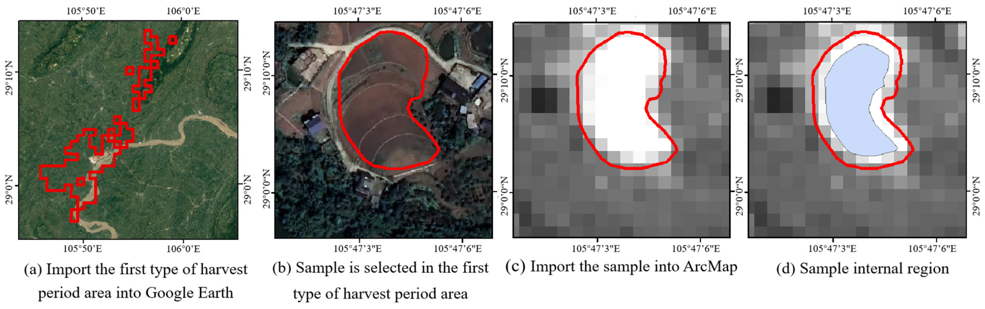
2.3.3. Rice Fields Extraction Model Construction and Application

Based on the unique features of large differences in vegetation between the pre-harvest and post-harvest periods of rice fields, the extraction model of rice fields was constructed using the following formula:

$${\mathrm{Diff}}_{\mathrm{NDVI}}={\mathrm{NDVI}}_{{\mathrm{t}}_1}- {\mathrm{NDVI}}_{{\mathrm{t}}_2}$$

(2)

where NDVI_t1 is the NDVI value of the preharvest period of rice fields, and NDVI_t2 is the NDVI value of the postharvest period of rice fields. To extract rice fields and determine the extraction threshold, if the NDVI values are greater than the threshold, they are classified as rice fields; otherwise, they are classified as other land types. To calculate the values of Diff_NDVI for different harvesting areas, according to the data sources shown in Table 1, Formula (2) was used. Due to the different harvesting periods in various regions, there were variations in the NDVI values of rice fields. To accurately and comprehensively extract rice fields, it was necessary to determine the threshold values of Diff_NDVI for different harvesting periods in respective regions. The threshold determination method primarily relied on historical Google imagery to statistically analyze the sample regions of Diff_NDVI for rice fields. Firstly, we imported the boundaries of different harvesting period regions into Google Earth Pro. Taking the first type of harvesting period region as an example (Figure 4a), we randomly selected 35 rice fields within the boundaries as samples (Figure 4b), and imported the samples back to ArcMap (Figure 4c). Because the sample regions’ boundaries were mixed pixels, to avoid their influence on threshold determination, buffer zones of 10 m (the pixel size of the Diff_NDVI) inside the boundaries were made. The buffer zones were removed from the rice fields in order to gain access to the interior of the sample regions (Figure 4d). Then, the mean and standard deviation of the Diff_NDVI within the interior of the sample regions in the rice fields were calculated. The samples were vector data, and the Diff_NDVI data were raster data. The means were subtracted from three times the standard deviations to calculate the thresholds. These thresholds were then utilized to extract the rice fields in their corresponding harvesting areas [32]. The rice fields extracted from different regions were finally merged to obtain a comprehensive dataset of rice fields for the study area spanning from 2019 to 2023. During the extraction process, slight variations in the thresholds may have resulted in the presence of small misclassified or isolated mixed pixels. Since subsequent studies relied on this data for analyzing drivers of rice field changes, it was imperative to minimize the impact of misclassification, mixing, and individual isolated pixels to demonstrate the overall trend in rice field changes. Thus, the data were processed using the raster fusion tool [33,34].

2.3.4. Temporal and Spatial Changes of Rice Fields

To explore the characteristics of rice field changes from 2019 to 2023, this study conducted an analysis from both temporal and spatial perspectives. The analysis involved using rice field transition matrices and rice field dynamic index calculations to assess temporal changes. Furthermore, spatial changes were analyzed by integrating DEM data. This comprehensive analysis allowed for the identification of pertinent characteristics and patterns in rice field changes.

Firstly, the land use transfer matrix can depict the transition of land types over different periods. It not only enables quantitative analysis of the specific quantity of conversions between land types, but also facilitates the analysis of their flow direction and composition [35]:

$${\mathrm{S}}_{\mathrm{ij}}=\left[\begin{array}{ccc}{\mathrm{S}}_{11}& \cdots & {\mathrm{S}}_{1\mathrm{n}}\\ ⋮& \ddots & ⋮\\ {\mathrm{S}}_{\mathrm{n}1}& \cdots & {\mathrm{S}}_{\mathrm{nn}}\end{array}\right]$$

(3)

where S represents the area, n represents the number of land types, and i and j represent the land types before and after the transfer, respectively.

Land use dynamics refers to the changes in the number of land use types over a specific period. It serves as an indicator of the intensity and speed at which land use changes occur, while also highlighting regional disparities [36]. It is divided into single land use dynamics and comprehensive land use dynamics. Due to the main focus of this study being on rice field changes, the land type was homogeneous, and a single land use dynamics approach was employed for analysis:

$$\mathrm{k}={\displaystyle \frac{{\mathrm{U}}_{\mathrm{b} }-{ \mathrm{U}}_{\mathrm{a}}}{{\mathrm{U}}_{\mathrm{b}}}}{\displaystyle \frac{1}{\mathrm{T}}} 100\%$$

(4)

k represents the dynamic degree of a certain land use type, U_b represents the area of a specific land use type at the end of a period, U_a represents the area of the same land use type at the beginning of the period, and T represents the time interval of change.

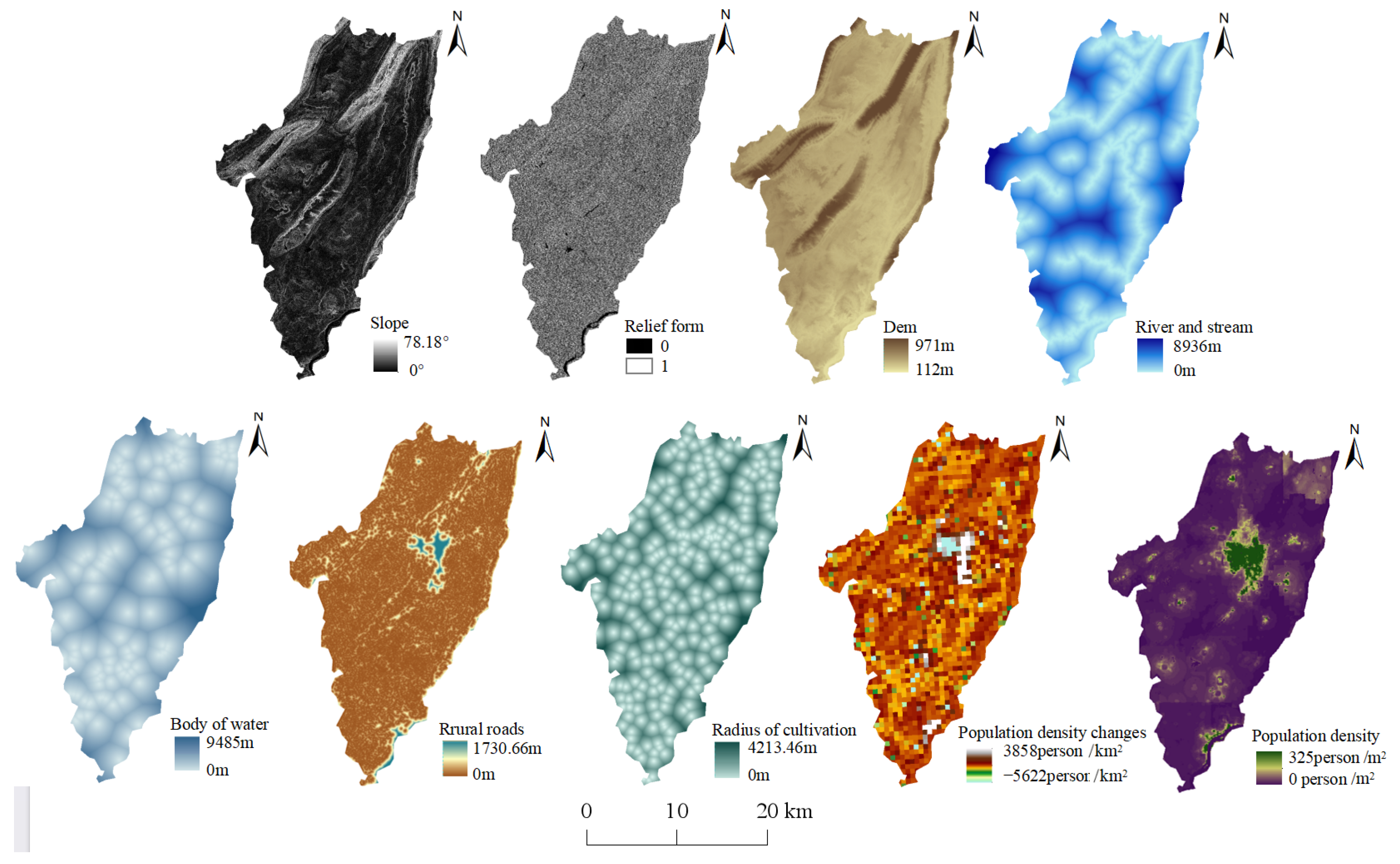
2.3.5. Analysis of Driving Forces of Rice Fields

Based on the analysis of spatiotemporal changes in rice fields over a five-year period, the logistic regression model was utilized to investigate the causes of these changes. The construction and analysis of the model are presented as follows:

(1) Model

The logistic regression model is used to analyze the relationship between the dependent variable and multiple explanatory variables. Depending on the number of dependent variables, it can be classified into binary and multinomial models [37,38]. Since the article explored the reasons behind the temporal and spatial changes in rice fields, the dependent variable in this study was whether the rice fields had changed from 2019 to 2023. When a change occurred, the dependent variable was assigned a value of 1, otherwise 0. Therefore, a binary logistic regression model was chosen, as shown in Equations (5) and (6):

$$\log ({\displaystyle \frac{{\mathrm{P}}_{\mathrm{i}}}{1 - {\mathrm{p}}_{\mathrm{i}}}})={\mathsf{\beta }}_0+{\mathsf{\beta }}_1{\mathrm{X}}_{1,\mathrm{i}}+{\mathsf{\beta }}_2{\mathrm{X}}_{2,\mathrm{i}}+...+{\mathsf{\beta }}_{\mathrm{n}}{\mathrm{X}}_{\mathrm{n},\mathrm{i}}$$

(5)

Formulas (4) and (5) were deduced to obtain P_i:

$${\mathrm{P}}_{\mathrm{i}}={\displaystyle \frac{\exp ({\mathsf{\beta }}_{0 }+{\mathsf{\beta }}_{\mathrm{i}}{\mathrm{X}}_{1,\mathrm{i}}+{\mathsf{\beta }}_2{\mathrm{X}}_{2,\mathrm{i} }+...+{\mathsf{\beta }}_{\mathrm{n}}{\mathrm{X}}_{\mathrm{n},\mathrm{i}})}{1+\exp ({\mathsf{\beta }}_0+{\mathsf{\beta }}_{\mathrm{i}}{\mathrm{X}}_{1,\mathrm{i}}+{\mathsf{\beta }}_2{\mathrm{X}}_{2,\mathrm{i}}+...+{ \mathsf{\beta }}_{\mathrm{n}}{\mathrm{X}}_{\mathrm{n},\mathrm{i}})}}$$

(6)

In the equation, P_i represents the probability of a certain land use type “i” occurring in each grid cell; β₀ is a constant, and “β” is a regression coefficient that measures the strength of the correlation between the driving factor and the land use type. The larger the value of “β”, the stronger the correlation; X_n,i represents the nth driving factor related to land use type “i”, and expβ represents the occurrence rate of the event.

(2) The Selection of Driving Factors

The spatial-temporal variations of rice fields are influenced by multiple factors, primarily classified into two main categories: natural factors and socio-economic factors. In terms of natural factors, considering the influences of geological landforms, water resources, and meteorological conditions, rice fields require suitable areas with appropriate slopes and terrain morphology for rice cultivation. Additionally, convenient irrigation is necessary to meet the water requirements for rice growth [39]. In terms of socioeconomic factors, compared to the influence mechanism of natural factors, the driving mechanisms brought about by social activities are more complex. These include regional economy, urbanization, the level of agricultural development, farmers’ willingness, population changes, and policy influences, among others [40]. However, due to factors such as the availability of data, the ability to quantify, consistency, variability, importance, and comprehensiveness [41], the driving factors used in this study were carefully considered from both natural and social perspectives, as depicted in

Table 4. Table of driving factors.

Variables		Types	Unit
Dependent variable	Gained Rice Fields	Binary classification	0, 1
	Lost Rice Fields	Binary classification	0, 1
Independent variable	Slope	Continuous classification	degree
	Terrain Morphology	Binary classification	0, 1
	Elevation	Continuous classification	m
	Distance From the River	Continuous classification	m
	Distance From the Water Body	Continuous classification	m
	Distance From the Road	Continuous classification	m
	Cultivation Radius	Continuous classification	m
	Population Density	Continuous classification	person/m2 (person/km2)

.

(3) Extraction of Dependent and Independent Variables.

Based on identifying the driving factors of the spatiotemporal changes in rice fields, relevant methods in ArcMap 10.6 were used to process the dependent and independent variable data for subsequent analysis using the logistic regression model. Before processing these variables, it is essential to standardize the spatial extent, coordinate systems, and spatial resolution of all data sources. This ensures the elimination of errors due to data inconsistencies, making the subsequent analysis more reliable and accurate, and also preventing errors during software operation.

For processing the dependent variables, based on rice field data from 2019 and 2023, the rice fields were defined as 1 using the reclassification tool, while other grids were defined as 0. Then, using the raster calculator, the reclassified rice field data for 2019 was subtracted from the rice field data for 2023, resulting in a raster map showing the changes in rice fields. Grids with a value of 1 represented gained rice fields, grids with a value of 0 represented unchanged land classes, and grids with a value of −1 represented lost rice fields. Finally, the rice field change chart was extracted as two separate raster charts, which were used as the dependent variables.

Then, the independent variables were extracted, including slope, terrain morphology, and elevation, which were all based on DEM data extraction. The slope was obtained using surface analysis tools. Terrain morphology is classified into positive and negative forms. Positive forms refer to terrain that rises relative to neighboring areas or newly uplifted regions, while negative forms refer to terrain that sinks relative to neighboring areas or newly subsiding regions [42]. The specific method involved analyzing the neighborhood to obtain the average elevation of the neighboring areas in the DEM. Then, using the raster calculator, the difference between the value of the area itself and its neighboring areas was calculated. If the difference was positive, it indicated positive terrain, while if it was negative, it indicated negative terrain. The rivers and rural roads were regarded as linear features and were analyzed using Euclidean distance; The water bodies were considered as polygon features and were converted into point features. Then, Euclidean distance analysis was conducted separately. Among these, the distance between residential settlements and rice fields represented the cultivation radius. As for the population density in the driving factors, LandScan and WorldPop are commonly used global population datasets. The LandScan dataset has a resolution of 1000 m × 1000 m and was updated until 2022, while the WorldPop dataset has a resolution of 100 m × 100 m and was updated until 2020. There are differences in both time and resolution between the two datasets, and in subsequent studies, all data need to be standardized to the same spatial resolution. Choosing different population datasets will result in different spatial scales involved in the subsequent analysis, leading to different suitability. Therefore, it was necessary to investigate separately and select the population dataset that had the best fit. For the LandScan dataset, population density change was used as the driving variable by subtracting the population density data of 2022 from that of 2019; As for the WorldPop dataset, population density was used as the driving variable based on the data from 2020.

After data processing, including the standardization of spatial extent, coordinate systems, and spatial resolution, the drive factor maps and rice field change maps were converted into ASCII format files. These files were then copied to the installation directory of the CLUE-S model. The rice field change files and driving factors files were transformed into unified record files using a conversion tool. During the conversion process, the no-data rasters were removed, and random sampling was performed. For data with a resolution of 100 m, random sampling was performed on 20% of the rasters to generate the samples. However, for data with a resolution of 1 km, all cells were selected due to the smaller number of cells. Finally, these samples were imported into SPSS Statistics for logistic binary regression analysis.

(4) Collinearity Diagnostics

There might be collinearity issues among the independent variables in the logistic regression model [43]. Therefore, before conducting binary logistic regression analysis, it is necessary to check for collinearity problems and remove them if found, as they can interfere with the accuracy of the regression results. Thus, the collinearity diagnostics were performed by selecting the “Analyze-Regression-Linear” option in SPSS Statistics, and multiple variance inflation factors (VIF) were obtained. When 0 < VIF < 10, it indicates the absence of multicollinearity. When 10 ≤ VIF < 100, it suggests the presence of moderate multicollinearity. When VIF ≥ 100, it indicates the existence of severe multicollinearity [44]. After conducting multicollinearity diagnosis on the 8 independent variables in this study, it was found that the VIF values range from 0 to 10, indicating the absence of multicollinearity. Hence, logistic binary regression analysis could be performed.

(5) Scale Effect Analysis

Based on various population datasets, this study established two spatial scales, namely 100 m and 1 km, for conducting logistic regression analysis. Then, based on the suitability value, the optimal spatial scale was selected for subsequent analysis. The driver maps and land use change maps at the two spatial scales were generated by resampling using the Resample tool. At the same time, ROC was selected as the criterion for selecting the optimal spatial scale. The ROC curve tool in SPSS Statistics was used to obtain the results. The test variable was set as the predicted probability, and the state variable was set as the dependent variable value, with values ranging from 0.5 to 1. The closer the value was to 1, the better the regression fit.

3. Results

3.1. Results of Spatial and Temporal Simulation of the Rice Harvesting Period

Through the analysis of time-series NDVI curves for various ground features in the sample area, it was found that the NDVI values of forests and grasslands are generally higher than those of other land categories. Rice fields and dry land have intermediate values, while construction land and water bodies have the lowest NDVI values. From 8 June to 5 July, the NDVI values of rice fields, forests and grasslands, and dry land all show upward trends, while the NDVI values of water bodies exhibit a downward trend. The NDVI values of construction land remain relatively unchanged. From 5 July to 11 August, the NDVI values of forests and grasslands, as well as dry land, continue to rise slightly. In contrast to earlier changes, the NDVI values of water bodies start to increase, while the NDVI values of construction land remain relatively stable. Unlike other ground features, the harvested rice fields experience a significant decrease in NDVI values from 5 July to 11 August, with a difference of 0.26. However, the NDVI values of non-harvested rice fields remain relatively stable. This indicates that the variation in NDVI values for rice fields during this period differs from other land types. For the rest of the period, the trends and degrees of change in NDVI values for all ground features are similar.

Therefore, rice fields were extracted based on the changes in NDVI between the pre-harvest and post-harvest periods. The harvest period was determined using a model constructed with altitude and latitude as indicators:

$$\mathrm{y}=8.077{ \mathrm{x}}_1+0.056 {\mathrm{x}}_2- 245.040$$

(7)

where x₁ is the latitude, x₂ is the altitude, and y is a value between the pre-harvest and post-harvest period of the rice fields. Substituting the altitude and latitude of a specific location into Equation (7) yields Y = 1, determining the rice harvest period for that location. Subsequently, the harvesting period range was simulated across the entire study area (see Figure 5). Figure 5 shows that the top left corner illustrates the range of the simulated rice harvest period in Chongqing. The range from −3 to 157 represents the harvest time, where Y = 1 indicates that the rice is harvested around August 1st, and so on. Since the distribution of rice was not known during the simulation of the harvest period, the simulation covers the entire area. Practical considerations revealed that regions classified as 7, 8, and 9—characterized by high elevations and forest cover—were unsuitable for rice cultivation. Therefore, these areas’ indicated harvesting periods were deemed impractical. However, this did not affect the subsequent extraction of rice fields because the core basis for rice extraction in this study was the change in NDVI values before and after the rice harvest. Therefore, even if certain areas that did not cultivate rice were simulated with a harvest period, they were not misclassified during extraction since the NDVI values in those areas did not exhibit the same changes as those in rice fields. For consistency in subsequent research, they were grouped into the 6th category, establishing the rice harvesting period in the study area from 31 July to 29 August. Figure 5 illustrates earlier rice harvesting in the southern region (first harvest zone category), contrasting with delayed harvesting in the northwestern region (categories 3 to 6). Additionally, the southeastern region predominantly falls into the second category, representing the largest harvested area during this period.

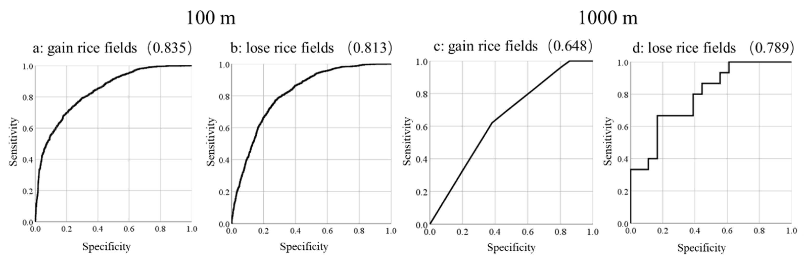
3.2. Precision Evaluation

The harvesting periods for each region were determined using the simulation model. Rice field distribution data from 2019 to 2023 were extracted based on the characteristic NDVI value decrease between pre-harvest and post-harvest periods. This study imported rice field data from 2019 to 2023 into ENVI 5.3. Stratified sampling was conducted using the “Select the Ground Truth Classification Image” function. A total of 1500 validation points were randomly generated each year, with 500 points generated for rice field layers and 1000 points for non-rice field layers. Validation points were visually interpreted based on historical Google imagery. The classification accuracy and Kappa coefficient were obtained by calculating the confusion matrix (

Table 5. Accuracy evaluation of rice fields classification results from 2019 to 2023.

Year	2019	2020	2021	2022	2023
Accuracy	0.95	0.92	0.93	0.94	0.92
Kappa	0.88	0.81	0.83	0.87	0.82

). From Table 5, it can be seen that the classification accuracy of rice fields over five years is 95%, 92%, 93%, 94%, and 92%, respectively, while the Kappa coefficients are 0.88, 0.81, 0.83, 0.87, and 0.82, respectively. On the other hand, when consulting the statistical yearbooks of the research area, it is observed that the rice cultivation area has been around 4 × 10⁴ hm² in recent years, slightly higher than the rice fields extracted in this study. This discrepancy can be attributed to various reasons. Firstly, rice field statistics data are primarily based on the area of the fields. However, in some instances, rice does not fully occupy the entire plot area, especially along the edges and in gaps, resulting in extracted data that are slightly lower than the recorded rice field statistics area. Secondly, the 10 m resolution of the data source in this study result in the inability to extract small and narrow rice fields within the research area. Finally, the statistical yearbook reports rely on farmers’ surveys for area estimations instead of actual measurements, thereby introducing errors.

3.3. Results of Rice Fields Extraction

(1) Overall Area Remains Stable with Pronounced Spatial Adjustments

Based on the NDVI difference method, the data of rice fields in the study area from 2019 to 2023 were obtained (Figure 6). From

Table 6. Changes in rice fields in different years of the study area.

Year	2019	2020	2021	2022	2023
Area (104 hm2)	3.74	3.78	3.78	3.79	3.81
Changes	gain (103 hm2)	1.74	1.75	1.49	1.58
	lose (103 hm2)	1.39	1.73	1.38	1.42
	net (hm2)	350	20	110	160
Dynamic degree (%)		0.93%	0.05%	0.29%	0.42%

and Figure 6, it can be observed that the total area of rice fields did not vary significantly each year. In terms of dynamics, the largest change in the area of rice fields occurred from 2019 to 2020, with a dynamic change rate of 0.93%. Conversely, the smallest change in the area of rice fields occurred from 2020 to 2021, with a dynamic change rate of 0.05%. This indicates that although the trend of changes in rice fields shows a characteristic of growth every year, the growth rate is relatively slow, overall presenting a state of basic stability. On the other hand, from Figure 6, it can be seen that the majority of the rice cultivation areas in the study area are distributed in flat terrain, showing a generally contiguous pattern. However, there are still some scattered rice fields.

Specifically, in 2019–2020, the influx of rice fields was 1.74 × 10³ $\mathrm{h}{\mathrm{m}}^2$, with an outflow of 1.39 × 10³ $\mathrm{h}{\mathrm{m}}^2$, resulting in a net increase of 350$\mathrm{h}{\mathrm{m}}^2$, marking the year with the largest net increase in rice field area over the past five years. In 2020–2021, the influx and outflow were 1.75 × 10³ $\mathrm{h}{\mathrm{m}}^2$ and 1.73 × 10³ $\mathrm{h}{\mathrm{m}}^2$, respectively, with a minor net increase of 20$\mathrm{h}{\mathrm{m}}^2$, indicating a year of minimal change in rice field area. However, the high inflow and outflow rates suggest significant spatial adjustments. In 2021–2022, the influx and outflow were 1.49 × 10³ $\mathrm{h}{\mathrm{m}}^2$ and 1.38 × 10³ $\mathrm{h}{\mathrm{m}}^2$, respectively, resulting in a net increase of 110$\mathrm{h}{\mathrm{m}}^2$, slightly higher than the previous year. Despite this, the spatial changes were less pronounced overall. Finally, in 2022–2023, the influx and outflow were 1.58 × 10³ $\mathrm{h}{\mathrm{m}}^2$ and 1.42 × 10³ $\mathrm{h}{\mathrm{m}}^2$, respectively, showing a net increase of 160 $\mathrm{h}{\mathrm{m}}^2$, signifying a notable spatial change compared to the previous year. In summary, while the total rice field area remains stable annually, significant spatial adjustments continue, affecting approximately 3.0 × 10³ $\mathrm{h}{\mathrm{m}}^2$ of land types.

(2) Clear Differences in the Changing Regions

Overall, analyzing the changes in rice fields from 2019 to 2023 in the study area,

Table 7. Rice field change transition matrix for the study area from 2019 to 2023. $\mathrm{h}{\mathrm{m}}^2$.

2019	2023		Total for the year 2019
	Rice fields	Other land categories
Rice fields	3.46 × 104	2.84 × 103	3.74 × 104
Other land categories	3.54 × 103	1.17 × 105	1.21 × 105
Total for the year 2023	3.81 × 104	1.20 × 105	1.58 × 105

indicates a loss of 2.84 × 10³ $\mathrm{h}{\mathrm{m}}^2$ of rice fields and an inflow of 3.54 × 10³ $\mathrm{h}{\mathrm{m}}^2$. This indicates significant spatial changes in rice fields from 2019 to 2023. Analyzing the specific spatial distribution of inflow and outflow of rice fields, Figure 7 shows that the gained of rice fields are evenly distributed over the five years, while the majority of the lost rice fields are located in the western and eastern parts of the study area, particularly in the western direction, demonstrating clear regional differences. To further investigate the regional disparities, the DEM data were classified. However, since most of the rice fields were located in areas with lower altitudes, it was necessary to divide them into five categories using equal geometric intervals to better showcase the changing characteristics of rice fields at different altitudes (Figure 7). From Figure 7, it can be observed that the gained rice fields are located in the altitude ranges of 225 m to 289 m, and 289 m to 402 m. On the other hand, the lost rice fields are mostly located in the altitude range of 289 m to 402 m. Furthermore, the remaining areas are predominantly rivers and slopes. This indicates that the cultivation of rice is significantly influenced by altitude, with rice fields being generally located at lower altitudes both in the past and present. However, considering the inflow and outflow of rice fields, it can be observed that some rice fields are being shifted from higher altitude areas to lower altitude areas, suggesting a tendency for rice to prefer growing in lower-altitude regions.

3.4. Analysis of Driving Forces

The driving factors are shown in Figure 8. Logistic regression analysis was conducted at two scales, 100 m and 1 km, and ROC curves were obtained for each scale (Figure 9). From Figure 9, it can be observed that the ROC values for both the inflow and outflow of rice fields at the 100 m scale are higher than those at the 1 km scale. Therefore, in this study, the 100 m spatial scale was chosen as the optimal simulation scale, and regression analysis results were obtained.

Table 8. Logistic regression analysis results of the research area.

Driving Factors	Gained Rice Fields			Lost Rice Fields
	β	Wald	Exp(β)	β	Wald	Exp(β)
Slope	−0.080	157.180	0.923	0.001	9.541	1.001
Terrain Morphology	−	−	−	−0.355	19.356	0.701
Elevation	−0.007	131.579	0.993	−	−	−
Distance From the River	−0.0002	28.373	1.000	0.0004	301.636	1.000
Distance From the Water Body	−0.001	738.384	0.999	−	−	−
Distance From the Road	−0.003	80.544	0.997	−0.005	18.212	0.998
Cultivation Radius	−0.001	104.839	0.999	0.001	153.309	1.001
Population Density	−0.078	77.138	0.925	−0.099	30.584	0.906
Constant	5.596	650.826	269.239	0.192	1.308	1.212

presents the results of logistic regression analysis in the study area. The Wald value is often used to test the logistic regression coefficients, which can be used to screen out the factors driving land use change. The Wald value test assumes that the regression coefficient β = 0. If the Wald value is close to 1, the hypothesis is accepted, indicating that the independent variable is considered unrelated to the dependent variable. Conversely, upon a larger Wald value, the hypothesis is rejected, indicating a strong correlation between the independent variable and the dependent variable. The results reveal a strong correlation between the distance to water bodies, slope, elevation, and cultivation radius with the area of gained rice fields in this analysis. The regression coefficients for these variables are all negative, indicating that rice fields are more likely to occur in areas with convenient irrigation facilities, flat terrain, lower elevations, and proximity to residential areas. On the other hand, the distance to rivers, cultivation radius, population density, and topography are strongly correlated with the area of lost rice fields. The regression coefficients for the distance to rivers and cultivation radius are positive, while the coefficients for population density and topography are negative. This suggests that rice fields are more prone to disappear in areas with inconvenient irrigation facilities, far from residential areas, lower populations, and negative topography.

4. Discussion

(1) The Influence of External Factors

In the context of rice field extraction, researchers have assessed the efficacy of different features in rice field classification for extraction. The findings indicated that feature selection plays a critical role in achieving higher classification accuracy and that combining temporal and spectral features can result in precise rice classification [45]. Therefore, compared to traditional machine learning methods combined with phenological feature data for crop area extraction, specific phenological periods can be selected to reduce the number of indicators, and crop information can be extracted based on temporal and spectral features to achieve an accurate, fast, and convenient method for obtaining rice field information. This paper utilizes the NDVI difference method to extract rice fields. However, certain external factors can interfere with the variation in NDVI values, including extreme weather conditions and human activities, such as prolonged high temperatures, rainfall, irrigation, pumping, and other causes of changes [46,47]. These factors have a significant impact on NDVI values. However, the specific forms, timing, and magnitude of this impact are difficult to quantify. Scholars have leveraged the distinctive characteristics of various growth stages of rice fields, such as the water content in early growth stages and the changes in luxuriance from the tillering phase to the heading stage, to employ the) and the Normalized Difference Vegetation Index (NDVI) for swift and accurate rice field information extraction in Lai’an County, Anhui Province [48]. This model relies on specific phenological periods and a limited number of indicators for crop information extraction, thereby enhancing its versatility; although, NDVI and NDWI are susceptible to external interference. This paper did not employ effective methods to address this issue, which should be improved in future research.

(2) Limitations of Data Sources

The limitations of data sources primarily pertain to two aspects: spatial resolution and cloud cover. Firstly, the study area contains fragmented land parcels. The spatial resolution of remote sensing imagery imposes limitations, resulting in the presence of grid cells that include a mixture of different land use types, rather than solely contiguous cells of the same land use type. These grid cells are referred to as mixed pixels. Different land types exhibit varying NDVI values, leading to substantial fluctuations in the NDVI values of these mixed pixels. As a result, the accuracy of rice field extraction results is impacted. Meanwhile, a portion of the rice fields in the study area are located in sloped areas, which are narrow and elongated, making it difficult to extract these rice fields completely. On the other hand, the study area frequently encounters cloud cover in the image data, making it necessary to select cloud-free or minimally cloud-covered imagery to minimize the impact on the NDVI values. However, as this study requires the selection of remote sensing images during the pre-harvest and post-harvest periods of rice fields, some images are inevitably affected by clouds, thereby affecting the accuracy of rice field extraction. Dong et al. have developed an automated rice mapping system based on Landsat that utilizes the unique spectral characteristics of rice during flooding and transplanting stages, by utilizing a time series of Landsat images [49]. Son et al. have constructed NDVI data for rice from the panicle initiation stage to the ripening stages using MODIS images and have applied machine learning techniques to extract rice information [50]. However, the methods above and the models equally encounter challenges related to the presence of mixed pixels and cloud cover, which can negatively impact the accuracy of the results. Future research initiatives should aim to address these issues effectively and enhance the precision of rice field extraction. Finally, due to the launch of the Sentinel-2 satellite in 2015, combined with the aforementioned cloud and other issues, this study has only investigated data from 2018 to 2023. This four-year period is relatively short; therefore, it is necessary to expand the period in future research to make the results more reliable.

(3) Limitations of Driving Factors

Numerous factors influence the spatiotemporal changes in rice fields, encompassing macro-level elements such as urban planning, relevant policies, and socio-economic development [51,52]. However, this study focuses on factors such as roads and population density, which can partially reflect regional development, planning, and socio-economic conditions, but they are not comprehensive enough because these macro-elements are influenced by multiple factors and cannot be measured solely by a few indicators. But some factors in the research process are difficult to quantify or obtain accurate data. Siagian et al. [52] employed a sampling method to select interviewed households and conducted a household-level investigation on the primary factors affecting rice field changes. The findings indicated that factors such as conformity psychology and income fluctuations have a significant impact on farmers’ choices. At the same time, factors such as water quantity, temperature, and sunlight affect crop growth. Open-source software, such as Quantum Geographic Information System (QGIS) and System for Automated Geoscience Analysis (SAGA), has been used by some scholars, allowing for spatial and terrain analysis. Specialized open-source software like DIVA-GIS has also been used, which is well-suited for crop analysis and allows for the analysis of parameters critical to crop growth and survival [53]. Therefore, future research should also strengthen the analysis of these factors and further explore the factors influencing the spatiotemporal changes in rice fields.

(4) Shortcomings in Precision Evaluation

The accuracy assessment in this study was primarily conducted through stratified sampling, followed by random generation of validation points. Finally, a manual visual interpretation of historical Google images was performed to calculate the confusion matrix. Nevertheless, the presence of cloud cover, distortion, and image stitching issues in certain areas of the historical Google images can interfere with manual interpretation. Hence, it is essential to prioritize on-site inspections and validations to reinforce the on-site comparisons. Furthermore, employing a combination of multiple accuracy assessment methods can significantly improve the accuracy of the evaluation results.

5. Conclusions

This study extracted rice fields in Yongchuan District, Chongqing from 2019 to 2023 using the NDVI difference method based on Sentinel data. The changes in the rice fields were analyzed, and a logistic regression model was employed to conduct a driving force analysis. The following conclusions have been derived:

• A simulation model for the rice harvesting period can be established through multiple regression analysis using two indicators, altitude and latitude. This model allows for the rapid and effective acquisition of the rice harvesting periods in different areas, thereby determining the data sources necessary for extracting rice fields.
• The confusion matrix reveals that the overall accuracy of rice fields extraction for the period 2019 to 2023 is 95%, 92%, 93%, 94%, and 92%, respectively, while the corresponding Kappa coefficients are 0.88, 0.81, 0.83, 0.87, and 0.82. These findings demonstrate the effectiveness of the NDVI difference method in the extraction of rice fields.
• The total area of rice fields in the study area does not change significantly annually and remains relatively stable. However, there are still notable spatial adjustments, with an approximate change area of 3.0 × 10³ hm². Overall, the spatial distribution of gained rice fields is relatively uniform over the five years, while the lost rice fields are predominantly located in the western and eastern parts of the study area, particularly in the western direction, indicating significant regional variations. Combined with the analysis of elevation, it is found that rice cultivation is significantly influenced by elevation and rice tends to grow at lower altitudes.
• The results of the logistic regression analysis indicate that rice fields have a higher probability of occurring in areas characterized by convenient agricultural irrigation, flat terrain, lower elevation, and proximity to residential areas. In contrast, they are more likely to vanish in areas with inconvenient agricultural irrigation, long distance from residential areas, lower populations, and negative topography.

References

1. Ali, F.; Jighly, A.; Joukhadar, R.; Niazi, N.K.; Al-Misned, F. Current Status and Future Prospects of Head Rice Yield. Agriculture 2023, 13, 705. [Google Scholar] [CrossRef]
2. Jamwal, P.; Brown, R.; Kookana, R.; Drechsel, P.; McDonald, R.; Vorosmarty, C.J.; van Vliet, M.T.H.; Bhaduri, A. The Future of Urban Clean Water and Sanitation. One Earth 2019, 1, 10–12. [Google Scholar]
3. Yao, W.; Tong, Y.; Liu, Q.; Zang, H.; Yang, Y.; Qi, Z.; Zeng, S. Spatiotemporal change characteristics and trade trend of global rice production. J. South. Agric. 2022, 53, 1776–1784. [Google Scholar] [CrossRef]
4. Ming, S.; Tan, X.; Tan, J.; Jiang, L.; Wang, Z. Analysis of influencing factors of rice planting area evolution in Dongting Lake Area during 1987–2017. J. Nat. Resour. 2020, 35, 2499–2510. [Google Scholar] [CrossRef]
5. Li, Z.; Long, Y.; Tang, P.; Tan, J.; Li, Z.; Wu, W.; Hu, Y.; Yang, P. Spatio-temporal changes in rice area at the northern limits of the rice cropping system in China from 1984 to 2013. J. Integr. Agr. 2017, 16, 360–367. [Google Scholar] [CrossRef]
6. Liu, L.; Huang, J.; Xiong, Q.; Zhang, H.; Song, P.; Huang, Y.; Dou, Y.; Wang, X. Optimal MODIS data processing for accurate multi-year paddy rice area mapping in China. Gisci. Remote Sens. 2020, 57, 687–703. [Google Scholar] [CrossRef]
7. Gu, Y. Study on the Characteristics of Crop Planting in Karakax County of Xinjiang. Master’s Thesis, Xinjiang University, Ürümqi, China, 2022. [Google Scholar] [CrossRef]
8. Singh, P.K.; Nag, A.; Arya, P.; Kapoor, R.; Singh, A.; Jaswal, R.; Sharma, T.R. Prospects of Understanding the Molecular Biology of Disease Resistance in Rice. Int. J. Mol. Sci. 2018, 19, 1141. [Google Scholar] [CrossRef] [PubMed]
9. Cai, Y.; Lin, H.; Zhang, M. Mapping paddy rice by the object-based random forest method using time series Sentinel-1/Sentinel-2 data. Adv. Space Res. 2019, 64, 2233–2244. [Google Scholar] [CrossRef]
10. Tolba, R.A.; El-Shirbeny, M.A.; Abou-Shleel, S.M.; El-Mohandes, M.A. Rice Acreage Delineation in the Nile Delta Based on Thermal Signature. Earth Syst. Environ. 2020, 4, 287–296. [Google Scholar] [CrossRef]
11. Guan, X.; Huang, C.; Liu, G.; Meng, X.; Liu, Q. Mapping Rice Cropping Systems in Vietnam Using an NDVI-Based Time-Series Similarity Measurement Based on DTW Distance. Remote Sens. 2016, 8, 19. [Google Scholar] [CrossRef]
12. Tian, J.; Tian, Y.; Cao, Y.; Wan, W.; Liu, K. Research on Rice Fields Extraction by NDVI Difference Method Based on Sentinel Data. Sensors 2023, 23, 5876. [Google Scholar] [CrossRef]
13. Li, T.; Li, W. Research Progress on the Evolution of Maize Spatial Pattern and Its Influencing Factors in China. Chin. J. Agric. Resour. Reg. Plan. 2021, 42, 87–95. [Google Scholar] [CrossRef]
14. Nurfadila, J.S.; Baja, S.; Neswati, R.; Rukmana, D. Analysis of trends and driving factors for plantation crop production. Bulg. J. Agric. Sci. 2022, 28, 828–836. [Google Scholar]
15. Zhao, J.; Yang, X. Spatial patterns of yield-based cropping suitability and its driving factors in the three main maize-growing regions in China. Int. J. Biometeorol. 2019, 63, 1659–1668. [Google Scholar] [CrossRef]
16. Chang, J.; Lin, Z.; Gao, W.; Du, X. Spatiotemporal evolution and driving factors of soybean production in Sichuan Province. Chin. J. Eco-Agric. 2024, 32, 476–489. [Google Scholar] [CrossRef]
17. Li, Y.; Han, M.; Kong, X.; Wang, M.; Pan, B.; Wei, F.; Huang, S. Study on transformation trajectory and driving factors of cultivated land in the Yellow River Delta in recent 30 years. China Popul. Resour. Environ. 2019, 29, 136–143. [Google Scholar] [CrossRef]
18. Jiang, N.; Jia, B.; Song, Y. Driving Forces of Arable Land Change in Beijing Based on Logistic Regression Model. Arid Zone Res. 2017, 34, 1402–1409. [Google Scholar] [CrossRef]
19. Xu, Y.; McNamara, P.; Wu, Y.; Dong, Y. An econometric analysis of changes in arable land utilization using multinomial logit model in Pinggu district, Beijing, China. J. Environ. Manag. 2013, 128, 324–334. [Google Scholar] [CrossRef] [PubMed]
20. Xu, Y.; Zhang, P.; Zhou, B. Study on Landscape Zoning of Land Use Based on Shannon Diversity T-Test Method—A Case Study of Yongchuan Distinct of Chongqing. Chin. J. Agric. Resour. Reg. Plan. 2019, 40, 134–141. [Google Scholar] [CrossRef]
21. Su, Y. Study on Land Use Change and Landscape Ecological Risk Assessment in Yongchuan District of Chongqing Province. Master’s Thesis, Southwest University, Chongqing, China, 2021. [Google Scholar] [CrossRef]
22. Wu, X.; Zhang, H. Evaluation of ecological environmental quality and factor explanatory power analysis in western Chongqing, China. Ecol. Indic. 2021, 132, 108311. [Google Scholar] [CrossRef]
23. Baetens, L.; Desjardins, C.; Hagolle, O. Validation of Copernicus Sentinel-2 Cloud Masks Obtained from MAJA, Sen2Cor, and FMask Processors Using Reference Cloud Masks Generated with a Supervised Active Learning Procedure. Remote Sens. 2019, 11, 433. [Google Scholar] [CrossRef]
24. Yang, J. Agricultural Land Use and Crop Phenological Information Extraction Based on Sentinel-2 Single Interannual Time-Series Data. Master’s Thesis, Huazhong Agricultural University, Wuhan, China, 2023. [Google Scholar] [CrossRef]
25. Tatem, A.J. Comment: WorldPop, open data for spatial demography. Sci. Data 2017, 4, sdata20174. [Google Scholar] [CrossRef]
26. Mao, D.; Wang, Z.; Luo, L.; Ren, C. Integrating AVHRR and MODIS data to monitor NDVI changes and their relationships with climatic parameters in Northeast China. Int. J. Appl. Earth Obs. 2012, 18, 528–536. [Google Scholar] [CrossRef]
27. Gerardo, R.; de Lima, I.P. Applying RGB-Based Vegetation Indices Obtained from UAS Imagery for Monitoring the Rice Crop at the Field Scale: A Case Study in Portugal. Agriculture 2023, 13, 1916. [Google Scholar] [CrossRef]
28. Gao, Y.; Yang, S.; Chen, Z. Refined Agro-Climatic Zoning Atlas of Chongqing; Meteorological Press: Beijing, China, 2016. [Google Scholar]
29. Epule, E.T.; Peng, C.; Lepage, L.; Nguh, B.S.; Mafany, N.M. Can the African food supply model learn from the Asian food supply model? Quantification with statistical methods. Environ. Dev. Sustain. 2012, 14, 593–610. [Google Scholar] [CrossRef]
30. Yu, Q. Refinement of Agro-Climatic Resources Simulation Method in Chongqing. Master’s Thesis, Chongqing Normal University, Chongqing, China, 2009. [Google Scholar]
31. Zhao, R.; Li, Y.; Chen, J.; Ma, M.; Fan, L.; Lu, W. Mapping a Paddy Rice Area in a Cloudy and Rainy Region Using Spatiotemporal Data Fusion and a Phenology-Based Algorithm. Remote Sens. 2021, 13, 4400. [Google Scholar] [CrossRef]
32. Liu, J.; Hu, J.; Ye, Y. Mathematical Expectations and Their Applications of Standard Deviations of Normal Population Samples. Coll. Math. 2019, 35, 83–88. [Google Scholar]
33. Wang, S.; Li, Q.; Wang, H.; Zhang, Y.; Du, X.; Gao, L. A Winter Wheat Drought Index based on TROPOMI Solar-Induced Chlorophyll Fluorescence. Arid Zone Res. 2021, 36, 1057–1071. [Google Scholar] [CrossRef]
34. Dong, W.; Yang, J.; Li, C.; Kong, F. Research on Effects of Multi-scale Map Generalization Based on Cellular Automaton. Bull. Surv. Mapp. 2014, 63–65. [Google Scholar] [CrossRef]
35. Yuan, Z.; Zhou, L.; Sun, D.; Hu, F. Impacts of Urban Expansion on the Loss and Fragmentation of Cropland in the Major Grain Production Areas of China. Land 2022, 11, 130. [Google Scholar] [CrossRef]
36. Wang, Z.; Shi, P.; Shi, J.; Zhang, X.; Yao, L. Research on Land Use Pattern and Ecological Risk of Lanzhou-Xining Urban Agglomeration from the Perspective of Terrain Gradient. Land 2023, 12, 996. [Google Scholar] [CrossRef]
37. Shamsi, R.; Ghasami, S. Relationship between decision changes under the study of random response (RR) using the logistic regression model. Eur. Phys. J. Plus. 2022, 137, 956. [Google Scholar] [CrossRef]
38. Zhang, C.; Zhou, Z.; Zhu, C.; Chen, Q.; Feng, Q.; Zhu, M.; Tang, F.; Wu, X.; Zou, Y.; Zhang, F.; et al. Analysis of the Evolvement of Livelihood Patterns of Farm Households Relocated for Poverty Alleviation Programs in Ethnic Minority Areas of China. Agriculture 2024, 14, 94. [Google Scholar] [CrossRef]
39. Wang, C.; Zhang, Z.; Zhang, J.; Tao, F.; Chen, Y.; Ding, H. The effect of terrain factors on rice production: A case study in Hunan Province. J. Geogr. Sci. 2019, 29, 287–305. [Google Scholar] [CrossRef]
40. Chandio, A.A.; Jiang, Y.; Ahmad, F.; Adhikari, S.; Ul Ain, Q. Assessing the impacts of climatic and technological factors on rice production: Empirical evidence from Nepal. Technol. Soc. 2021, 66, 101607. [Google Scholar] [CrossRef]
41. Jiao, D. Regional Land Use Evolvement and Simulation Research Driven by Sino-Russian Border Trade. Ph.D. Thesis, China University of Geosciences, Beijing, China, 2017. [Google Scholar]
42. Li, J.; Zhang, H.; Xu, E. A two-level nested model for extracting positive and negative terrains combining morphology and visualization indicators. Ecol. Indic. 2020, 109, 105842. [Google Scholar] [CrossRef]
43. Assaf, A.G.; Tsionas, M. Testing for Collinearity using Bayesian Analysis. J. Hosp. Tour. Res. 2021, 45, 1131–1141. [Google Scholar] [CrossRef]
44. Chennamaneni, P.R.; Echambadi, R.; Hess, J.D.; Syam, N. Diagnosing harmful collinearity in moderated regressions: A roadmap. Int. J. Res. Mark. 2016, 33, 172–182. [Google Scholar] [CrossRef]
45. Singha, M.; Wu, B.; Zhang, M. Object-Based Paddy Rice Mapping Using HJ-1A/B Data and Temporal Features Extracted from Time Series MODIS NDVI Data. Sensors 2017, 17, 10. [Google Scholar] [CrossRef]
46. Xie, X.; He, B.; Guo, L.; Miao, C.; Zhang, Y. Detecting hotspots of interactions between vegetation greenness and terrestrial water storage using satellite observations. Remote Sens. Environ. 2019, 231, 111259. [Google Scholar] [CrossRef]
47. Zhao, A.; Zhang, A.; Liu, J.; Feng, L.; Zhao, Y. Assessing the effects of drought and “Grain for Green” Program on vegetation dynamics in China’s Loess Plateau from 2000 to 2014. Catena 2019, 175, 446–455. [Google Scholar] [CrossRef]
48. Yang, Y.; Huang, Y.; Tian, Q.; Wang, L.; Geng, J.; Yang, R. The Extraction Model of Paddy Rice Information Based on GF-1 Satellite WFV Images. Spectrosc. Spect. Anal. 2015, 35, 3255–3261. [Google Scholar] [CrossRef]
49. Dong, J.; Xiao, X.; Kou, W.; Qin, Y.; Zhang, G.; Li, L.; Jin, C.; Zhou, Y.; Wang, J.; Biradar, C.; et al. Tracking the dynamics of paddy rice planting area in 1986-2010 through time series Landsat images and phenology-based algorithms. Remote Sens. Environ. 2015, 160, 99–113. [Google Scholar] [CrossRef]
50. Son, N.; Chen, C.; Chen, C.; Guo, H.; Cheng, Y.; Chen, S.; Lin, H.; Chen, S. Machine learning approaches for rice crop yield predictions using time-series satellite data in Taiwan. Int. J. Remote Sens. 2020, 41, 7868–7888. [Google Scholar] [CrossRef]
51. Garcia De Jalon, S.; Iglesias, A.; Quiroga, S.; Bardaji, I. Exploring public support for climate change adaptation policies in the Mediterranean region: A case study in Southern Spain. Environ. Sci. Policy 2013, 29, 1–11. [Google Scholar] [CrossRef]
52. Siagian, D.R.; Shrestha, R.P.; Shrestha, S.; Kuwornu, J.K.M. Factors Driving Rice Land Change 1989-2018 in the Deli Serdang Regency, Indonesia. Agriculture 2019, 9, 186. [Google Scholar] [CrossRef]
53. Valjarevic, A.; Popovici, C.; Stilic, A.; Radojkovic, M. Cloudiness and water from cloud seeding in connection with plants distribution in the Republic of Moldova. Appl. Water Sci. 2022, 12, 262. [Google Scholar] [CrossRef]
Figure 1. The location and topography of the study area.
Agriculture 14 01165 g001
Figure 2. (a) Unmanned aerial remote sensing images of various ground feature samples at different time periods within the study area. (b) NDVI images of various ground feature samples at different time periods within the study area.
Agriculture 14 01165 g002
Figure 3. The time-series NDVI curves for major types of ground feature samples in the study area.
Agriculture 14 01165 g003
Figure 4. Rice field threshold determination—sample example.
Agriculture 14 01165 g004
Figure 5. Numerical simulation of rice harvesting periods in the study area.
Agriculture 14 01165 g005
Figure 6. Rice fields extraction results from 2019 to 2023.
Agriculture 14 01165 g006
Figure 7. Changes in rice fields from 2019 to 2023.
Agriculture 14 01165 g007
Figure 8. Various driving factors.
Agriculture 14 01165 g008
Figure 9. ROC curves for changes in rice fields.
Agriculture 14 01165 g009