A Comparative Study of Different Dimensionality Reduction Algorithms for Hyperspectral Prediction of Salt Information in Saline–Alkali Soils of Songnen Plain, China

Abstract

Hyperspectral technology is widely recognized as an effective method for monitoring soil salinity. However, the traditional sieved samples often cannot reflect the true condition of the soil surface. In particular, there is a lack of research on the spectral response of cracked salt-affected soils despite the common occurrence of cohesive saline soil shrinkage and cracking during water evaporation. To address this research, a laboratory was designed to simulate the desiccation cracking progress of 57 soda saline–alkali soil samples with different salinity levels in the Songnen Plain of China. After completion of the drying process, spectroscopic analysis was conducted on the surface of all the cracked soil samples. Moreover, this study aimed to evaluate the predictive ability of multiple linear regression models (MLR) for four main salt parameters. The hyperspectral reflectance data was analyzed using three different band screening methods, namely random forest (RF), principal component analysis (PCA), and Pearson correlation analysis (R). The findings revealed a significant correlation between desiccation cracking and soil salinity, suggesting that salinity is the primary factor influencing surface cracking of saline–alkali soil in the Songnen Plain. The results of the modeling analysis also indicated that, regardless of the spectral dimensionality reduction method employed, salinity exhibited the highest prediction accuracy for soil salinity, followed by electrical conductivity (EC) and sodium (Na⁺), while the pH model exhibited the weakest predictive performance. In addition, the usage of RF for band selection has the best effect compared with PCA and Pearson methods, which allows salt information of soda saline–alkali soils in Songnen Plain to be predicted precisely.

1. Introduction

Soil salinization is a significant form of soil degradation that results in alterations to the physical, chemical, biological and hydrological properties of soil [1,2,3]. This detrimental process not only hinders normal plant growth and weakens crop yield and quality [4], but it also has adverse implications for the construction of engineering facilities and land development [5], thereby posing a major obstacle to the national economy. Presently, saline soil of China is predominantly found in arid and semiarid regions, accounting for nearly one-tenth of the world’s saline soil area. This equates to approximately 4.88% of the available land in China [6]. The Songnen Plain, characterized by its unique climate and terrain, is one of the largest salt–alkaline soil areas in China [7]. The high concentration of soluble salts in this region further degrades its physicochemical properties, thus impeding plant growth and development and ultimately jeopardizing food security and the ecological system. Consequently, it is imperative to engage in precise, rapid, and non-destructive measurement techniques for assessing soil salinity in the Songnen Plain. Such initiatives are crucial for effectively ameliorating salt-affected soils, which also hold great significance for both local economic and environmental development.

The conventional techniques for determining salt parameters of salinized soil involve field measurements and laboratory analysis. One commonly used method is electromagnetic induction, which measures soil conductivity by analyzing primary and secondary magnetic fields [8]. However, electromagnetic induction instruments like the EM-38 are expensive and sensitive to environmental factors, affecting the reliability of results [9,10]. Although laboratory analysis provides accurate salt parameter measurements [11], the process can damage the soil surface and has a noticeable delay in obtaining results. Remote sensing has emerged as a valuable tool for monitoring the spatial distribution and temporal changes of salinized soil due to its wide coverage and frequent observations [12,13,14]. Nevertheless, this technique faces challenges, including the mixed pixel problem and low spectral resolution, which hinder the establishment of a precise quantitative relationship between spectral features and soil salinity. In conclusion, while field positioning and laboratory analysis have been traditionally employed for soil salinity assessment, the use of remote sensing has become prevalent due to its broad coverage and frequent monitoring. Nonetheless, improving the accuracy and reliability of remote sensing-based salinity assessment remains a challenge.

Hyperspectral remote sensing has emerged as a crucial method for quantitatively extracting soil salinity due to its wide band range and high spectral resolution, which has garnered significant attention from scholars. Li et al. [15] conducted an analysis of the spectral characteristics of saline soil samples in different states, including powdered, agglomerated, and cracked. They confidently identified the spectral sensitive bands of soda sodic soil as 990 nm, 1470 nm, 1990 nm, and 2170 nm. Moreover, they also observed a significant decrease in spectral reflectance with increasing soil salinity. Hu et al. [16] employed random forest regression to evaluate the importance of variables in 62 hyperspectral bands. They identified the most significant bands for predictive modeling of soil salinity in bare ground, dense vegetation, and sparsely vegetated areas as 610 nm, 650 nm, and 870 nm, respectively. Mandal et al. [17] effectively characterized the spectral features of soil salinity and discovered distinctive reflectance in the bands 427 nm, 487 nm, 950 nm, 1414 nm, 1917 nm, 2206 nm, 2380 nm, and 2460 nm. In another study, Das et al. [18] utilized an airborne imaging spectrometer to measure the spectral properties of agricultural areas in India with varying salinity levels. They identified four significant absorption spectral intervals, including 937–1017 nm, 1198–1253 nm, 1438–1533 nm, and 2139–2230 nm, which could be effectively utilized for accurate prediction of soil total salinity. Overall, these studies highlight the importance of hyperspectral remote sensing in extracting and predicting soil salinity, providing valuable insights into the spectral characteristics and sensitive bands associated with different salinity levels.

Although it is possible to achieve high accuracy in the inversion of hyperspectral data, several challenges arise, including the issues of large data volume, noticeable redundancy in the data, and slow processing speed. Additionally, variations in soil composition, physical and chemical properties, measuring conditions, and surface conditions can significantly impact the diagnostic spectral characteristics utilized in the hyperspectral inversion of soil parameters. Consequently, it becomes imperative to carefully select suitable spectral features to enhance the predictive ability of the model, while also reducing computational complexity. In the research on spectral dimensionality reduction and spectral feature selection, many scholars focused on principal component analysis (PCA), Pearson correlation analysis (R), and random forest (RF). Specifically, Wang et al. [19] used first derivative analysis and PCA to downscale raw hyperspectral data, afterward they developed an estimation model for soil salt ions and mapped the spatial distribution of salt content. Pan et al. [20] applied PCA to reduce the dimensionality of the entire spectrum and established a prediction model for soil texture, their results also showed that PCA dimensionality reduction can effectively achieve nonlinear interactions between multiple spectral components, which also can be well applied to modeling and predicting soil particle size. Cui et al. [21] used Pearson correlation analysis to assess the significance of 20 commonly used spectral indices on the UAV platform, and then developed three machine-learning regression models for efficient agricultural soil salinity monitoring. Bangelesa et al. [22] used variable importance projection and recursive feature selection methods for feature selection in partial least squares regression and RF and found that the spectral reflectance from 400 to 700 nm can be used to predict the content of soil organic matter. Ge et al. [23] estimated soil salinity in Da’an City using Landsat 8 imagery, their results indicated that the model developed with RF for variable selection achieved better prediction accuracy than the that developed using the full wavelength range.

Although spectral features have the potential to capture disparities in soil salinity to a certain extent, previous studies mainly relied on ground and sieved soil samples for spectral measurements. Additionally, spectral data extracted from large-scale hyperspectral remote sensing images often faced the challenge of mixed pixels, rendering them inadequate representations of true surface conditions of saline soil. Although desiccation cracking of cohesive saline–alkali soil during water evaporation has been well studied as a natural occurrence, there has been limited research on measuring hyperspectral data of cracked soil surfaces. Furthermore, prediction models for regional soil salinity based on hyperspectral remote sensing inversion, considering desiccation cracks, are also severely lacking. In pursuit of this objective, spectral characteristics based on cracked soil surfaces were measured and analyzed, an in-depth investigation will be subsequently undertaken into methods for screening spectral features and developing inversion models for the main salt parameters. Such findings will thus provide fundamental theoretical support for the application of hyperspectral remote sensing in soil salinity monitoring and enhance the understanding of spectroscopy in China.

2. Material and Method

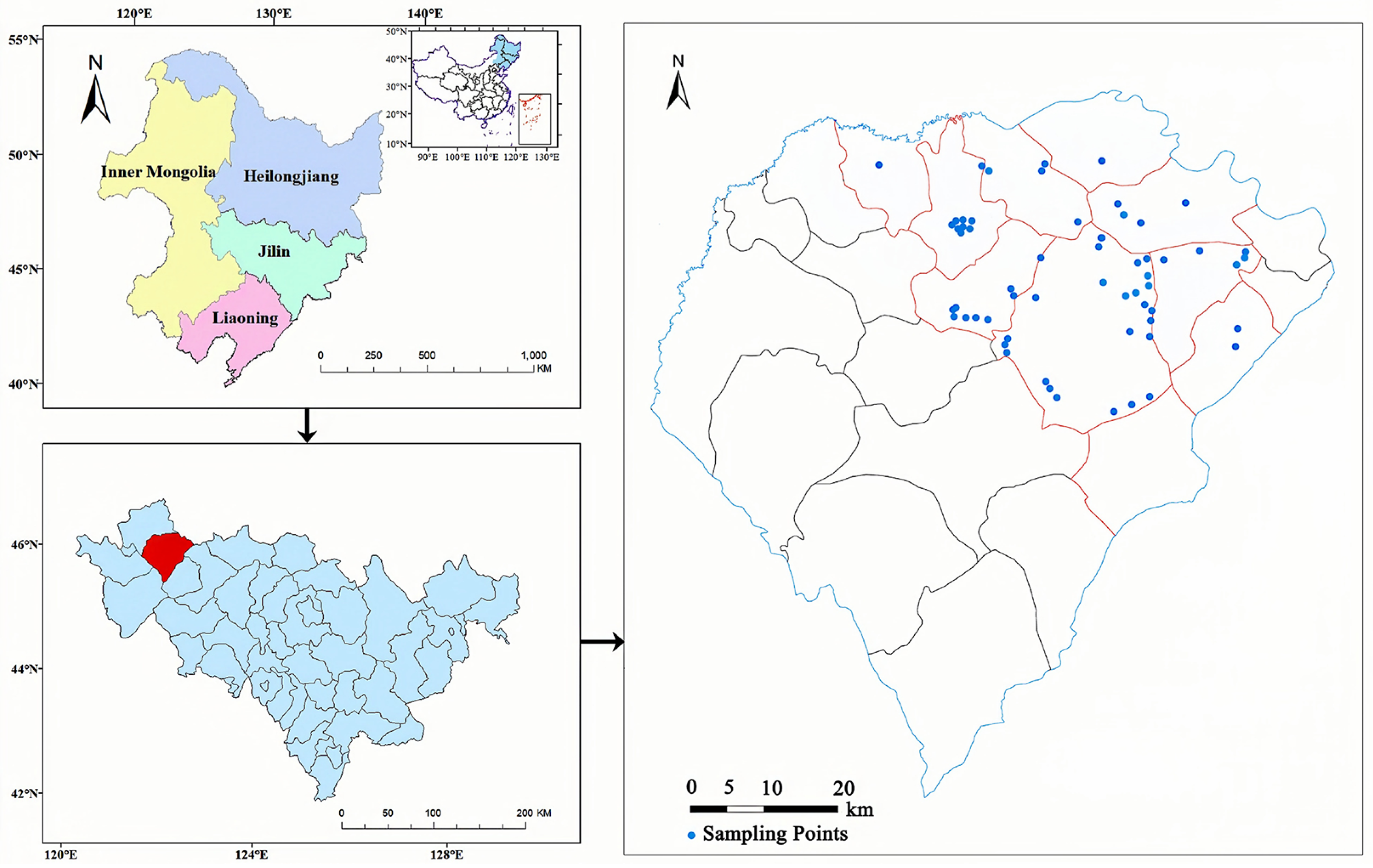
2.1. Study Area

The saline–alkali soil in the western part of Songnen Plain covers a vast area of approximately 3.73 × 106 km² with the dominant salt minerals of carbonates (Na₂CO₃) and bicarbonates (NaHCO₃) [24,25], is considered to be one of the three typical soda saline distribution areas globally. Da’an City, situated within this region, experiences a typical temperate continental climate. The city witnesses extreme annual temperatures, with the minimum recorded as −35 °C and the maximum as 36.9 °C. On average, the temperature remains around 4.5 °C. Precipitation in the area heavily concentrates during the months of July and August, contributing to an average annual rainfall of around 400 mm. In contrast, the average annual evaporation reaches up to 1900 mm. This significant disparity between evaporation and precipitation, combined with the unique geographical features, hydrogeological conditions, and unsustainable human activities like overgrazing, logging, and unreasonable cultivations (such as poor drainage [26], excessive irrigation water [27], excessive soil compaction [28], etc.), contributes to severe soil salinization in the region [29]. To account for the variation in soil salinity levels and surface cracking conditions in the field, a total of 57 sampling points were carefully chosen. These sampling points fell within the geographical coordinates longitude 123°42′33″ E to 124°6′1″ E and latitude 42°23′57″ N to 45°39′57″ N (as displayed in Figure 1). For all sampling points, soil samples (20 kg for each) were collected from the top 20 cm of the soil and then subjected to drying, grounding, and sieving through a 2 mm sieve in the laboratory. The processed soil samples were divided into two parts to measure soil physicochemical parameters and conduct the controlled desiccation cracking experiment.

2.2. Soil Property Measurements

The soil characteristics measured in this study primarily consisted of soil pH, electrical conductivity (EC), the concentrations of major ions in saline soils, and the distribution of particle sizes. Note that the measurement of SO₄²⁻ was excluded from the study due to its low concentration in the Songnen plain [30,31]. To measure the soil pH and EC, a soil suspension with a soil–water mass ratio of 1:5 was prepared and analyzed using potentiometric and conductometric methods, respectively [32,33]. The ion concentrations in the soil samples were determined by using soil extract with the same water-soil mass ratio of 5:1. Specifically, the Cl⁻ concentration was determined through titration with an AgNO₃ solution, while the HCO₃⁻ and CO₃²⁻ concentrations were measured using the double indicator neutralization method. The Na⁺ and K⁺ contents were measured using a flame photometer, and the Mg²⁺ and Ca²⁺ were determined using the EDTA titration method. It should be noted that the total salinity refers to the sum of all ion concentrations. In addition, the particle size distribution of the soil samples was also analyzed in this study using the Mllvern MS-200 laser particle size analyzer.

2.3. Soil Surface Cracking Experiments

To simulate the process of water loss and subsequent desiccation cracking on the surface of soda saline–alkali soil, a laboratory controlled test were carried out equally to all soil samples after considering the cracking experiment proposed by Zeng et al. [34] and Al-Jeznawi et al. [35]. Specifically, the soil samples were first prepared as a saturated slurry with a water content of 50%. These samples were then poured into wooden sample boxes with size of 50 cm × 50 cm × 3 cm. To ensure consistency, each sample was flattened using a spatula and weighed. Subsequently, the samples were placed in a laboratory setting to undergo a desiccation cracking test under controlled experimental conditions including a temperature of 25 °C, humidity of 35%, and pressure of 101 kPa. Once the mass of all soil samples no longer decreased, measurements of soil surface cracking were taken under completely dry conditions. To accomplish this, a digital camera was installed on a fixed platform, with the camera lens positioned vertically downwards from a height of 1 m above the ground. A rectangular area, measuring 50 cm on each side, was marked on the ground. It was ensured that the intersection point of the rectangular diagonal coincided with the center of the camera projection. To maintain consistency among the images, the camera settings including white balance, shutter speed, and aperture were set identically for each photograph. Finally, each soil sample was placed within the marked rectangular area and photographed. Additionally, a chessboard calibration plate, with a side length of 50 cm, was also photographed, which served the purpose of providing geometric correction to the crack images for accurate measurements of crack features.

2.4. Crack Feature Extraction

After the completion of the desiccation cracking process, a standardized preprocessing approach (Figure 2) was employed to process the crack images. First, a polynomial-model-based geometric distortion correction was applied to each crack image. Subsequently, the images were cropped to a size of 50 cm × 50 cm and converted to grayscale. Since the cracks exhibited distinct differences in gray values from the surrounding background, a histogram thresholding method was utilized to determine the optimal separation threshold for the cracks. In order to focus solely on the cracks, the grayscale image was then subjected to binarization and inverse operations. Subsequently, skeletonization was performed until the cracks reduced to a width of one pixel. The preprocessed images were then utilized to extract the crack length (CL) and crack area (CA) of each image. For the calculation of CL, the skeletonized image of each crack sample was employed to quantify the number of skeletal pixels. By knowing the actual size of one pixel, the crack length could be accurately calculated. Regarding CA, the crack ratio of each sample was determined using the equation R = n/N, where n represents the total number of crack regions in the binary image and N denotes the total number of image elements. Consequently, the actual area of each crack sample was obtained using the formula CA = 2500 × R cm².

2.5. Spectra Measurement

Spectroscopy analysis was performed on stabilized cracked soil samples in order to examine their spectral response. After the desiccation cracking test was fully completed, spectroscopy was conducted by using a field portable hyperspectral spectrometer known as ASD Field Spec 3, which consists of two detectors such as the visible near-infrared detector (VNIR: 350–1000 nm, sampling interval of 1.4 nm and spectral resolution of 3 nm) and short-wave infrared detector (SWIR: 1000–2500 nm, sampling interval of 2 nm and spectral resolution of 10 nm). For further analysis purposes, the spectrometer was resampled to a higher resolution of 1 nm. The spectral measurements of the soil samples were all carried out under weather conditions that were clear and cloudless. To extract the reflectance values from the cracked surface of soda saline–alkali soils, a light probe with a 25° field of view was fixed in a vertically downward position on a 1 m high platform (Figure 3).

In this particular investigation, the ASD spectrometer was utilized to measure a circular area with a diameter of 45 cm at the center of each cracked sample (as depicted in Figure 4). Prior to obtaining the spectra for each sample, a dark current removal process was implemented [36], followed by calibration using a whiteboard [37]. The actual soil reflectance was then calculated by spectrometer automatically using the following equation [38].

$$\mathrm{R}(\mathsf{\lambda })={\displaystyle \frac{\mathrm{S}(\mathsf{\lambda })-\mathrm{D}(\mathsf{\lambda })}{\mathrm{W}(\mathsf{\lambda })-\mathrm{D}(\mathsf{\lambda })}}$$

(1)

where R(λ) is the real reflectance of the soil sample at wavelength λ, S(λ) is the detector response at wavelength λ, D(λ) is the detector response of the dark current at wavelength λ, and W(λ) is the detector response value of the white calibration at wavelength λ. Subsequently, the average of 10 reflectance measurements was determined for each soil sample, serving as the final spectral data. It is important to highlight that, in this study, a Gaussian model was adopted for spectral resampling at intervals of 10 nm. This procedure aimed to mitigate reflectance noise and achieve data compression, all while maintaining the morphological characteristics of the reflection curve to a substantial extent. Moreover, specific spectral bands within the ranges of 1350–1420 nm, 1800–1920 nm, and 2360–2500 nm were deliberately excluded in order to minimize any confounding effects stemming from atmospheric moisture [39,40].

2.6. Dimensionality Reduction

2.6.1. Random Forest Algorithm

Random forest (RF) is a machine learning algorithm introduced by Breiman in 2001 [41]. It is based on the Bagging method and involves extracting multiple samples from the input data with replacement. These subsamples are then used as training sets to construct individual decision trees. At each leaf node of a decision tree, a random selection of features is made for training purposes, and the best split point based on this feature set is chosen to divide the subtree into its left and right branches. Furthermore, the importance of each feature is estimated using out-of-bag data (OOB), resulting in a reduction of the dimensionality of the independent variables [42]. To mitigate the risk of overfitting, decision trees are built in parallel, introducing randomness into the algorithm and ultimately yielding a robust model capable of accurately predicting outcomes [43]. In this study, the implementation of this process predominantly relied on the random forest package in R software (version 4.3.2).

2.6.2. Principal Component Analysis

Principal component analysis (PCA) is a widely utilized linear dimensionality reduction technique that transforms high-dimensional data into low-dimensional representations while preserving the essential information of the original data. The essence of PCA lies in mapping the original data onto a new coordinate system via a linear transformation, aiming to maximize the data’s variance under the new coordinates. In this research, we employed MATLAB software (2023a) to implement PCA. Initially, the original data is standardized to eliminate scaling discrepancies among different features. Subsequently, the covariance matrix of the standardized data is calculated to ascertain the interrelationships between individual features. Next, the principal components of the data are determined by computing the eigenvalues and eigenvectors of the covariance matrix. Furthermore, the first k principal components are selected based on the criterion that the cumulative contribution rate surpasses 95%. The score coefficients of each principal component are computed using Equation (2).

$${\mathrm{e}}_{\mathrm{i}}={\displaystyle \frac{{\mathrm{\alpha }}_{\mathrm{i}}}{\sqrt{{\mathrm{\lambda }}_{\mathrm{i}}}}}$$

(2)

where e_i describes the score of each principal component, α_i represents the variable loadings corresponding to each principal component, and λ_i refers to the eigenvalues corresponding to each principal component.

2.6.3. Correlation Analysis

In order to quantitatively analyze the relationship between each soil salinity parameter and the reflectance of different wavelength bands, the Pearson correlation coefficient was calculated using the following equation.

$$\mathrm{R}={\displaystyle \frac{{\displaystyle \sum _{\mathrm{i}=1}^{\mathrm{n}}({\mathrm{x}}_{\mathrm{i}}-\overline{\mathrm{x}}})\times ({\mathrm{y}}_{\mathrm{i}}-\overline{\mathrm{y}})}{\sqrt{{\displaystyle \sum _{\mathrm{i}=1}^{\mathrm{n}}({\mathrm{x}}_{\mathrm{i}}-\overline{\mathrm{x}})}\times {\displaystyle \sum _{\mathrm{i}=1}^{\mathrm{n}}({\mathrm{y}}_{\mathrm{i}}-\overline{\mathrm{y}})}}}}$$

(3)

where x_i refers to the salt parameter and y_i represents the reflectance at a certain band. In order to better illustrate the relationship between salt parameters and spectral characteristics, correlation coefficient curves in the whole band range were plotted in this study.

2.7. Multivariate Linear Model

As a fast and simple prediction method, multiple linear regression (MLR) has the advantage of removing multicollinearity and autocorrelation among variables. This study aims to assess the accuracy of different feature band screening algorithms for predicting the main parameters in cracked soils. MLR models were thus developed using feature variables screened by three algorithms (RF, PCA, and R). The MLR model takes the following basic form:

$$\mathrm{y}={\mathsf{\beta }}_0+{\mathsf{\beta }}_1{\mathrm{x}}_1+{\mathsf{\beta }}_2{\mathrm{x}}_2+\cdots +{\mathsf{\beta }}_{\mathrm{k}}{\mathrm{x}}_{\mathrm{k}}+\mathsf{\epsilon }$$

(4)

where y is a certain salt parameter, x_k refers to the spectral index, β_k represents the regression coefficient, and ε describes the random error.

2.8. Accuracy Evaluation

To evaluate fitting and generalization ability of all the developed models, evaluation indexes such as R², RMSE, and MAE were used in this study. The formulas for these indexes are listed as follows:

$${\mathrm{R}}^2={\displaystyle \frac{{\displaystyle \sum _{\mathrm{i}=1}^{\mathrm{n}}({\widehat{\mathrm{y}}}_{\mathrm{i}}-\overline{\mathrm{y}}}{)}^2}{{\displaystyle \sum _{\mathrm{i}=1}^{\mathrm{n}}({\mathrm{y}}_{\mathrm{i}}-\overline{\mathrm{y}}}{)}^2}}$$

(5)

$$\mathrm{R}\mathrm{M}\mathrm{S}\mathrm{E}=\sqrt{{\displaystyle \frac{{\displaystyle \sum _{\mathrm{i}=1}^{\mathrm{n}}{({\widehat{\mathrm{y}}}_{\mathrm{i}}-{\mathrm{y}}_{\mathrm{i}})}^2}}{\mathrm{n}}}}$$

(6)

$$\mathrm{M}\mathrm{A}\mathrm{E}={\displaystyle \frac{1}{\mathrm{n}}}{\displaystyle \sum _{\mathrm{i}=1}^{\mathrm{n}}\left|{\widehat{\mathrm{y}}}_{\mathrm{i}}-{\mathrm{y}}_{\mathrm{i}}\right|}$$

(7)

where ${\widehat{\mathrm{y}}}_{\mathrm{i}}$ describes the predicted value, y_i is the measured value, and n is the number of soil samples.

In order to enhance the credibility of the accuracy of the validation set of different salinity parameter prediction models. Leave-one-out cross-validation (LOOCV) was introduced in this study for the accuracy validation of different prediction models. LOOCV represents a limiting case of k-fold cross-validation (KCV), which is a general approach used to evaluate the predictive performance of a statistical model in the absence of new data [44]. Specifically, for a dataset of N samples, it is divided into n equal-sized parts (n = N). For each iteration, only one sample is used for testing and the remaining samples are used for training, the iterations are continuously computed until all the samples are used as one test set [45]. After all the iterations are completed, the overall accuracy of the dataset is finally calculated.

3. Result

3.1. Soil Parameters

Table 1. Statistical description of physical and chemical parameters of soil samples.

Soil Parameters	Min	Max	Mean	SD	CV (%)	Skewness	Kurtosis
pH	8.01	10.77	9.83	0.73	7.41	−1.14	0.18
EC (ds/m)	0.06	3.39	0.97	0.84	86.64	1.02	0.56
Na+ (mg/g)	0.12	14.12	3.32	3.28	98.95	1.51	2.13
K+ (mg/g)	0.01	0.06	0.02	0.01	67.41	2.14	5.49
Ca2+ and Mg2+ (mg/g)	0.10	1.60	0.53	0.32	59.75	1.19	1.67
HCO3− (mg/g)	0.12	5.00	1.57	0.99	63.4	1.11	1.38
CO32− (mg/g)	0	5.50	1.75	1.56	89.33	1.02	0.14
Cl− (mg/g)	0.08	5.25	1.32	1.46	110.44	1.34	0.86
Salinity (mg/g)	1.06	29.73	8.50	6.46	75.98	1.22	1.43
ESP (%)	0.26	47.30	10.58	9.91	93.67	1.67	3.43
Clay (%)	25.39	32.04	27.98	1.54	5.49	0.43	−0.27
Silt (%)	28.72	40.40	35.19	3.18	9.03	−0.12	−0.82
Sand (%)	28.26	43.94	36.85	3.64	9.87	−0.21	−0.85

N = 57; SD: standard deviation; CV: coefficient of variation.

presents the physicochemical parameters obtained from the soil samples collected in this study. The pH values in the study area ranged from 8.01 to 10.77, and the ESP values ranged from 0.26% to 47.3% with an average of 10.58%, indicating alkaline soil according to the classification criteria proposed by USSLS in 1954. Furthermore, the dominant cation in the study area was Na⁺, which exhibited considerably higher levels compared to K⁺, Ca²⁺, and Mg²⁺. Although the difference in the content of the three anions was not as pronounced as that of the cations, the anions were mainly concentrated in CO₃²⁻ and HCO₃⁻. Moreover, the coefficients of variation (CV) of all soil salt parameters (excluding pH) exceeded 59.75%, indicating that the selected soil samples were well-representative and could accurately depict the distribution of soil salinity in the study area. In addition to the chemical properties, the particle size distribution measurements demonstrated limited variation in soil texture across all samples. Clay, silt, and sand exhibited narrow ranges with low CV values of 5.49%, 9.03%, and 9.87%, respectively.

Figure 5 displays the cross-correlations among various salt parameters for the 57 soil samples. The figure reveals that salinity exhibited the strongest correlation coefficient with EC and Na⁺ concentrations, suggesting a close relationship between these variables. Additionally, salinity demonstrated moderate correlations with Cl⁻, CO₃²⁻, and HCO₃⁻, indicating some degree of association. In contrast, the correlations between salinity and K⁺, Ca²⁺, and Mg²⁺ were weak, suggesting a limited connection. Moreover, Figure 5 also highlights the absence of significant correlations between Ca²⁺ and Mg²⁺ with K⁺, as well as their poor associations with other salt parameters. Among the anions, Cl⁻, CO₃²⁻, and HCO₃⁻ exhibited low correlations with all other salt parameters, except for their strong relationships with EC, salinity, and Na⁺. This study specifically focuses on salinity, EC, and Na⁺, as they display the highest correlations with salt parameters. Despite a correlation coefficient of only 0.64 between pH and total salinity, the inclusion of pH in the analysis is crucial due to its significance in characterizing soil alkalinity.

3.2. Crack Parameters

Table 2. Statistical description of crack parameters in soil samples.

Crack Parameters	Min	Max	Mean	SD	CV (%)	Skewness	Kurtosis
CL (cm)	200.00	797.18	444.26	120.65	27.16	0.54	0.58
CA (cm2)	36.78	547.54	311.80	130.80	41.95	−0.08	−0.78

N = 57; CL: crack length; CA: crack area; SD: standard deviation; CV: coefficient of variation.

displays the crack parameters extracted from the soil samples following the drying process. The results revealed a wide range of crack parameters for CL, ranging from 200.00 cm to 797.18 cm, and for CA, ranging from 36.78 cm² to 547.54 cm². The coefficient of variation (CV) values for CL and CA were 27.16% and 41.95%, respectively. Additionally, the standard deviation (SD) values for CL and CA were 120.65 and 130.80, respectively. These findings indicated significant differences in the crack characteristics among the soil samples, suggesting that these characteristics effectively differentiated the level of cracking in the soil samples.

Table 3. Correlation coefficients between crack parameters and main soil parameters.

	pH	EC	Na+	K+	Ca2+ & Mg2+	HCO3−	CO32−	Cl−	Salinity	Clay	Silt	Sand
CL	0.66	0.92	0.91	−0.25	0.25	0.62	0.76	0.83	0.94	0.14	0.23	−0.26
CA	0.45	0.55	0.50	−0.28	0.08	0.47	0.31	0.50	0.52	0.26	0.04	−0.15

N = 57; CL: crack length; CA: crack area.

provides the results of the correlation analysis between the crack parameters and soil parameters. It was evident from the table that the crack parameters exhibited positive correlations with all soil parameters, except for K⁺ and sand content in the soil. The correlation between CL and each soil parameter is notably higher than that of CA. Furthermore, the crack length demonstrated a strong correlation with salinity, EC, and the concentration of Na⁺, with correlation coefficients exceeding 0.9. However, there was no apparent relationship between the crack length and the concentrations of K⁺, Ca²⁺, and Mg²⁺. Moreover, the correlations between the crack parameters and soil texture parameters are relatively weak for both CL and CA.

3.3. Spectral Characteristics

Figure 6 shows the spectral reflectance curves of 57 cracked soil samples. It can be observed that the majority of soil samples displayed similar curve shapes, but noticeable differences were still observed. Specifically, the reflectance curves exhibited a consistent increasing trend within the wavelength range of 350–1350 nm. In the range of 1420–1800 nm, the slope of the reflectance curves appeared to be lower compared to the previous range, resulting in a stabilization of the reflectance curves and a slowdown in the rate of increase. Between 1920 and 2360 nm, the changes in reflectance were more intricate: an increase was observed from 1920 to 2130 nm, followed by a prominent reflectance peak at approximately 2130 nm. Subsequently, the curves exhibited a decrease in reflectance from 2130 to 2200 nm and gradually reached a state of stabilization thereafter. Notably, Figure 6 also demonstrates that the reflectance curves of all cracked soil samples predominantly reached their highest point around 1350 nm, suggesting the presence of salt minerals such as NaHCO₃ and Na₂CO₃ with distinct spectral characteristics. This observation highlights the significant variations in the spectral reflectance curves of cracked soil samples.

3.4. Screening Results of Spectroscopy

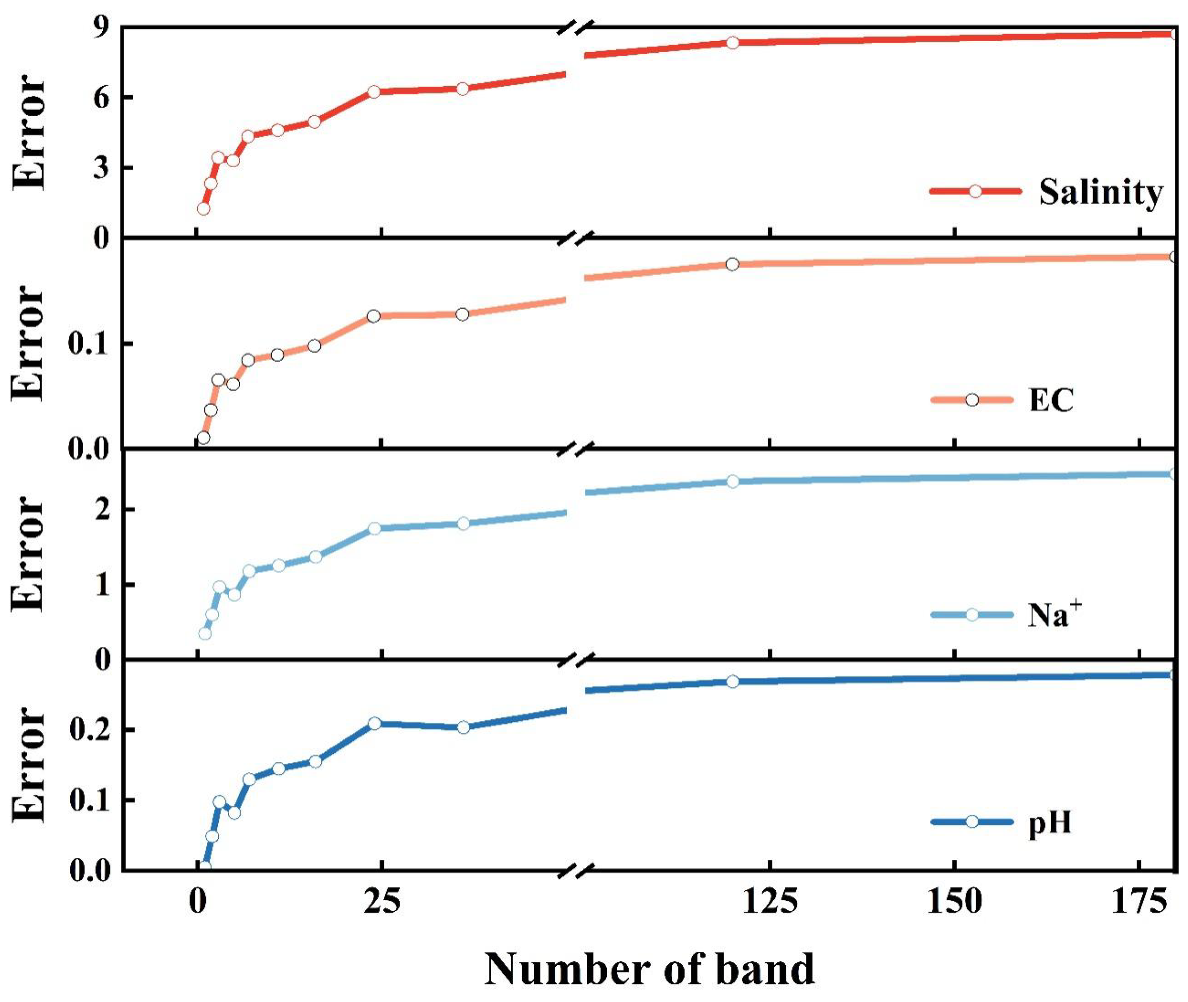
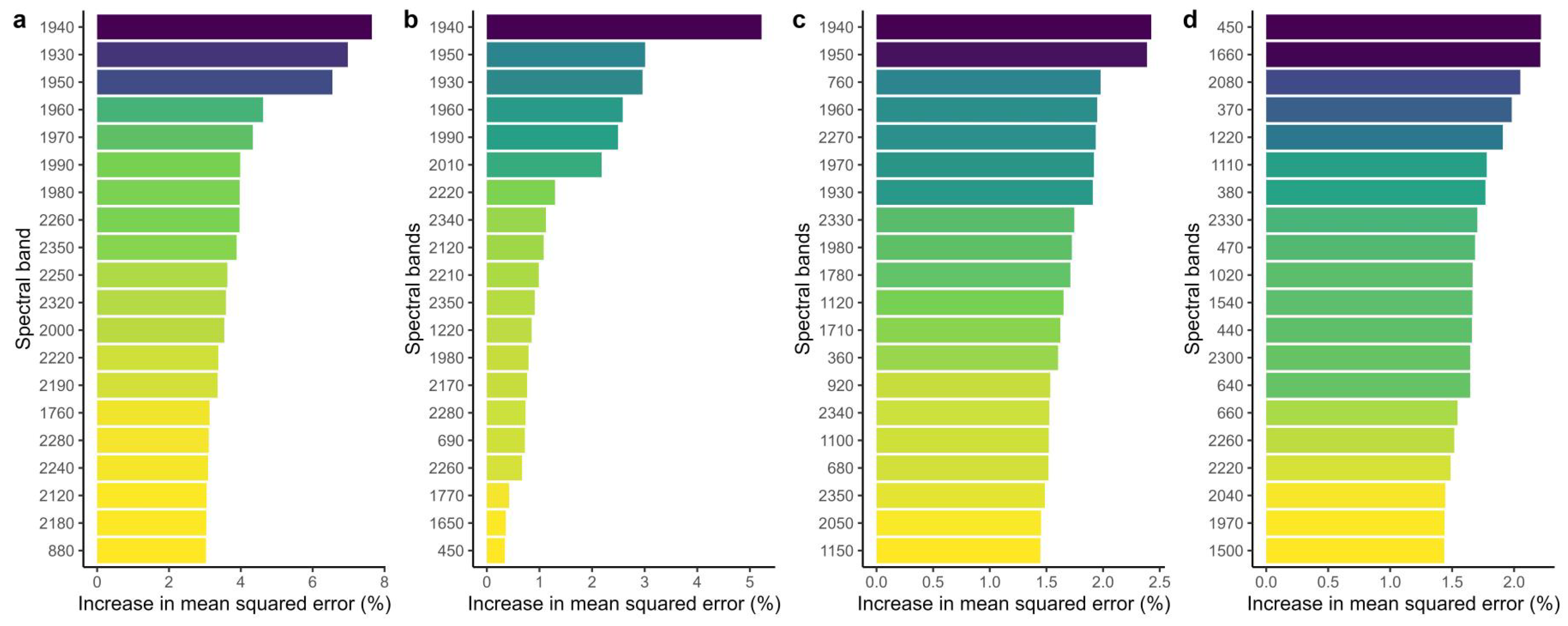
3.4.1. Random Forest Algorithm

In this study, RF modeling was conducted using spectral reflectance data and main salt parameters (salinity, EC, Na⁺, and pH). Before modeling the RF model, 10-fold cross-validation tests with 5 replications were conducted first in order to better evaluate the performance of the RF algorithm and determine the number of optimal spectral bands (Figure 7). From the figure, it can be seen that for the four main salt parameters, the RF model was optimal, with the smallest error when the number of selected characteristic bands was 5.

After the RF model established, the optimal bands were selected based on their contribution to each salt parameter, which was determined by the percentage increase in mean squared error. Figure 8 illustrates the top 20 spectral bands that made the greatest contribution to each salt parameter. The salinity model exhibited the highest accuracy with 409 decision trees, wherein the top 5 bands were identified as B₁₉₄₀, B₁₉₃₀, B₁₉₅₀, B₁₉₆₀, and B₁₉₇₀. As for EC, the RF model achieved the best accuracy with 56 decision trees, and the top 5 bands were B₁₉₄₀, B₁₉₅₀, B₁₉₃₀, B₁₉₆₀, and B₁₉₉₀. With regard to Na⁺, the RF model demonstrated the best accuracy with 40 decision trees, and the top 5 bands contributing the most were B₁₉₄₀, B₁₉₅₀, B₇₆₀, B₁₉₆₀, and B₂₂₇₀. However, the accuracy of the algorithm proved to be poor in predicting pH with 141 decision trees, and the corresponding top 5 bands were B₄₅₀, B₁₆₆₀, B₂₀₈₀, B₃₇₀, and B₁₂₂₀.

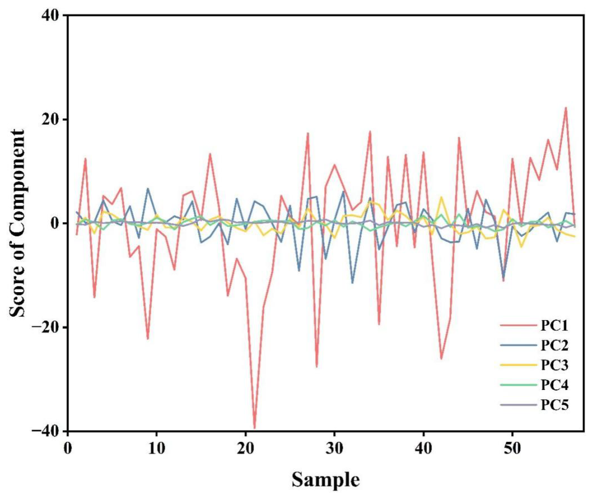
3.4.2. Principal Component Analysis

In this study, the PCA algorithm was applied to downscale 180 bands of hyperspectral data from cracked soil samples, following the processing steps outlined in Section 2.6.2. To facilitate a more robust comparison with the RF and correlation coefficient curves, five principal components were selected to screen the bands with results presented in

Table 4. Principal component contribution table.

Component	Total	Contribution Rate (%)	Cumulative Contribution Rate (%)
1	159.62	88.68	88.68
2	15.92	8.85	97.53
3	3.54	1.96	99.49
4	0.60	0.33	99.82
5	0.16	0.09	99.91

, which includes the eigenvalues and contribution rates of the initial five principal components. The presented table demonstrates that the cumulative contribution of these components reached 99.9%, indicating that they successfully captured the essential spectral characteristics of the original data.

Figure 9 presents the score values of the five principal components in all soil samples, which represented the numerical values of each principal component for the original data points and were considered as the results of dimensionality reduction from hyperspectral reflectance data.

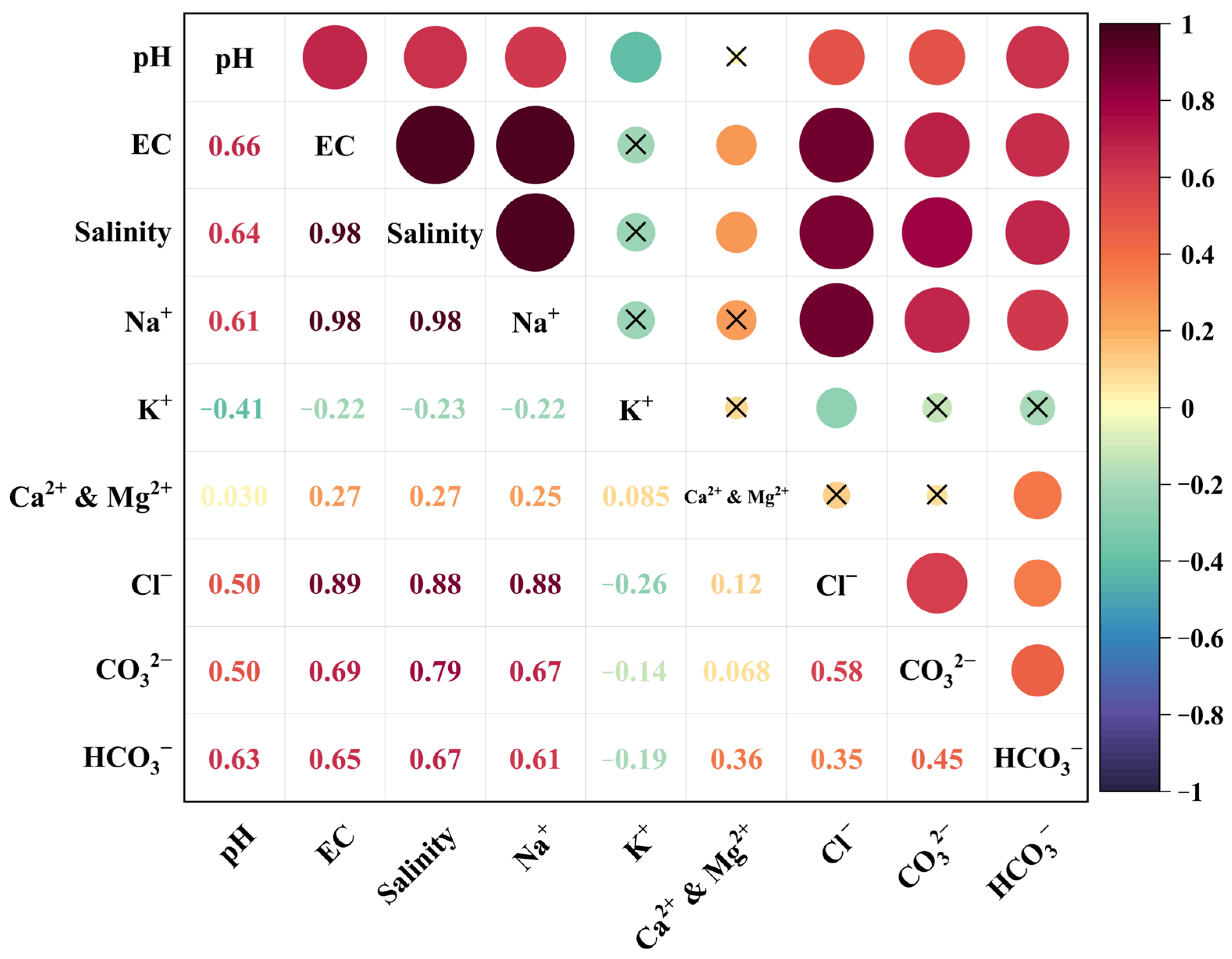
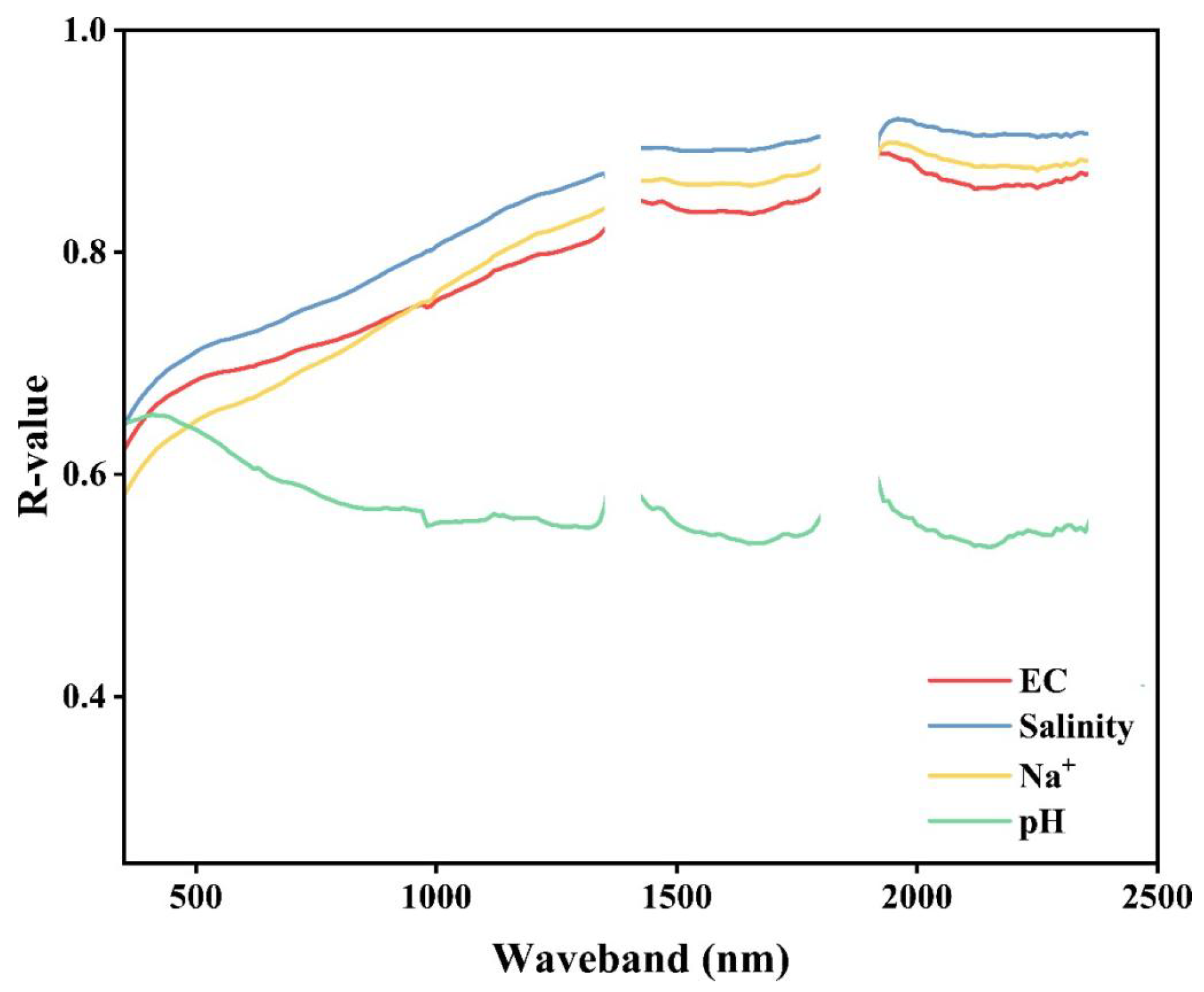
3.4.3. Pearson Correlation Coefficients

Figure 10 illustrates the correlation curves between reflectance and the main salt parameters over the entire spectral band from 350 to 2500 nm. It is evident from the graph that the correlation curves of the salt parameters exhibited a discernible pattern, with salinity, Na⁺, EC, and pH roughly arranged in the order of significance. Remarkably, EC, salinity, and Na⁺ demonstrate elevated values as the wavelengths venture towards the longer end in the visible and near-infrared spectra. Conversely, pH showcased an inverse correlation trend with diminished correlation coefficients observed at longer wavelengths. The correlation coefficients of the four salt parameters in the ranges of 1420–1800 nm and 1920–2360 nm showed a decreasing and then increasing trend. In order to further improve the selection of characteristic bands through correlation curve algorithms and establish prediction models with the four salt parameters, the correlation curves were combined with the diagnostic spectral characteristics of the two main salt minerals of NaHCO₃ and Na₂CO₃, resulting in the identification of five characteristic bands in order of importance including B₁₄₇₀, B₁₉₉₀, B₂₁₇₀, B₉₉₀, and B₁₃₄₀.

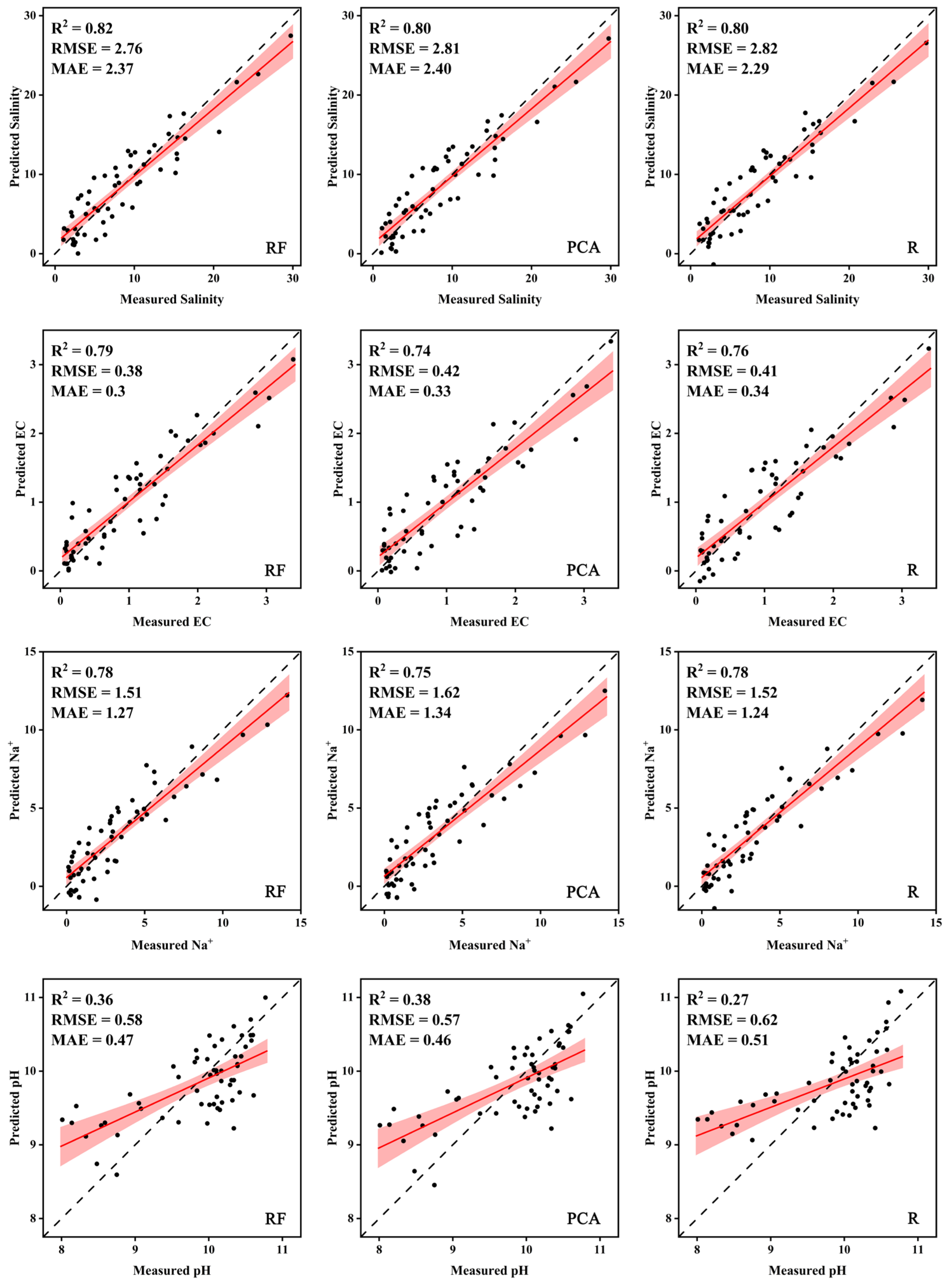
3.5. Multiple Linear Regression Models

Prediction Models

Table 5. The results of band screening.

Salt Parameters	Filtering Algorithm	Characteristic Band
——	PCA	PC1 (X1), PC2 (X2), PC3 (X3), PC4 (X4), PC5 (X5)
——	R	B1470 (X1), B1990 (X2), B2170 (X3), B990 (X4), B1340 (X5)
Salinity	RF	B1940 (X1), B1930 (X2), B1950 (X3), B1960 (X4), B1970 (X5)
EC		B1940 (X1), B1950 (X2), B1930 (X3), B1960 (X4), B1990 (X5)
Na+		B1940 (X1), B1950 (X2), B760 (X3), B1960 (X4), B2270 (X5)
pH		B450 (X1), B1660 (X2), B2080 (X3), B370 (X4), B1220 (X5)

PCA: principal component analysis, R: correlation coefficient, RF: random forest.

presents a summary of the band screening results obtained from hyperspectral data analysis for four salt parameters utilizing three algorithms. It is important to note that the PCA algorithm does not consider any salt parameter during its calculation process. Consequently, the characteristic bands identified by the correlation curves pertaining to the salt parameters remain consistent. Therefore, the characteristic bands for the four salt parameters identified by these two algorithms can be regarded as identical.

In order to improve the credibility of the salt prediction model, the LOOCV method was used to verify the accuracy of the salt prediction model. Specifically, all samples were sorted according to the order of data collection. Afterward, 56 samples were selected as training to build a multiple linear regression model, and the remaining one was used as validation to obtain the predicted values. The process was repeated 57 times until the predicted values of all samples were obtained. Finally, the overall assessment of the model accuracy was made based on the predicted and measured salt parameters.

To provide a more comprehensive understanding of the variations in models generated by different screening algorithms, scatter plots were utilized to compare the predicted values of the four salt parameters with their corresponding measured values (Figure 11). Regarding the prediction of total soil salinity, the three dimensionality reduction algorithms exhibited comparable accuracy, with R² values all above 0.8. Additionally, variations in model accuracy can be observed with respect to the electrical conductivity (EC) value. Notably, the highest accuracy, with an R² of 0.79 and an RMSE value of 0.38, was achieved through the RF method. On the other hand, the PCA algorithm yielded the lowest accuracy, which was reflected in an R² of 0.74 and an RMSE value of 0.42, resulting in an R² difference of approximately 0.05. Concerning sodium ions (Na⁺), all three reduction algorithms yielded similar R² from 0.75–0.78. However, the model developed using RF stood out due to its smaller RMSE value. In terms of pH prediction, the MLR models developed utilizing all three spectral screening methods performed poorly, resulting in low R² values ranging from only 0.46 to 0.51. From the comparison of the three downscaling algorithms, it can be seen that although the modeling accuracy between the various dimensionality reduction algorithms slightly varied, RF can be considered the most stable with highest accuracy for the total salinity, EC value, and Na⁺, while the prediction accuracy of pH was poor regardless of the dimensionality reduction methods.

4. Discussion

Desiccation cracking is a complex process influenced by various factors, including thickness, texture, salinity, temperature, and soil moisture [46,47,48]. Cracks on the surface of saline soils are commonly observed due to higher evaporation rates compared to precipitation. Previous studies have highlighted the significant role of clay content in the formation of cracks in saline soils. For instance, Cheng et al. [49] conducted cracking tests on two types of clays and found a strong correlation between clay content and soil cracking tensile strength. Similarly, Mu et al. [50] examined three loess soils with different clay contents and demonstrated that clay content significantly impacts both shrinkage and drying cracking patterns of soils. However, in this study, the effect of clay content on the complete process of saline soil cracking was relatively small due to the limited range of clay content in our soil samples. This finding is consistent with the research conducted by Zhang et al. [51], who investigated the basic properties of saline soils in the Songnen Plain. Their study revealed that the composition of clay minerals, such as illite and kaolinite, had minimal influence on the drying and cracking process of saline soil. Furthermore, numerous studies have indicated that the type and content of salt minerals greatly affect soil cracking behavior [52,53,54], which were also considered to be the primary factors influencing soil cracking in this study. Throughout the cracking process, the Songnen Plain experiences significant soil moisture evaporation due to high evaporation rates. As water evaporates, salts migrate upwards and accumulate on the soil surface, forming a water-binding film between soil particles with a high concentration of soluble cations, particularly Na⁺ ions with large hydrolysis radii. Increased soil salt concentration leads to decreased stability of soil aggregates [55]. Consequently, the distance between soil particles increases, weakening the cementation between particles and reducing the tensile strength of the soil samples [56]. When the tensile stress in the soil exceeds its tensile strength, surface cracks form and subsequently shrink and crack.

Desiccation cracks exert a substantial influence on the spectral characteristics of saline-alkali soil as they induce variations in the soil crust and roughness, thereby directly affecting its reflectance. The presence of salinity amplifies the size of fractures, resulting in increased area scattering from the soil surface and volume dispersion within the cracks. Consequently, surface cracks expand in magnitude due to soil salinity, leading to enhanced area scattering from the soil surface and volume scattering within the cracked areas. This causes a decrease in the amount of energy received by the spectrometer, ultimately resulting in a decrease in reflectance. Moreover, the presence of cracks contributes to a complex surface morphology that intensifies the spectral disparities between soil samples with varying crack characteristics [57]. The heightened spectral differences on the surface of cracked soils, in comparison to uncracked soils, facilitate more accurate predictive modeling of soil properties through the utilization of spectral bands on the cracked soil surface. These findings aligned with previous studies conducted by Ren et al. and Dong et al. [39,58]. Notably, Ren et al. [39] investigated the impact of salt content on the spectral reflectance of soils, considering the influence of drying cracks in a sample set of 17 soils. They discovered that the correlation between spectral response of cracked soil samples and soil physicochemical properties was generally stronger than that of soil samples devoid of cracks. Additionally, Dong et al. [58] introduced the concept of cracking rate and constructed a model for satellite spectral inversion of soil EC, showcasing that the presence of cracks in saline soil affects satellite spectra. Moreover, considering these cracks during the modeling of saline soil inversion remarkably enhances the accuracy of the model. Therefore, when creating a regression model for salt parameters based on spectral response, integration of the cracked state of soil samples improves the realism of estimated values and elevates the predictive accuracy of the model.

The advancement of remote sensing technology has led to an increase in the application of geochemical property inversion. However, the full wavelength band is not suitable for predicting soil salinity parameters due to the large data volume, data redundancy, and slow processing speed and also suffers from an overfitting problem. Therefore, scientific and rational dimensionality reduction processing of hyperspectral data has been the research direction of hyperspectral computing. Nevertheless, previous research on soil salinity prediction modelling has primarily focused on the selection of algorithms for the prediction model. The dimensionality reduction processing of hyperspectral data frequently employs a single algorithm, without conducting a comparative analysis between different dimensionality reduction techniques. Therefore, one originality of this study is the examination of the diagnostic spectral characteristics of cracked salinized soil obtained by different importance algorithms. On this basis, the prediction effect of multiple linear regression models was compared and analyzed on soil salinity based on different screening methods. Specifically, three-dimensionality reduction algorithms were implemented and compared for downsizing hyperspectral data. Although principal component analysis (PCA) is a commonly used linear dimensionality reduction method for inverting soil properties with hyperspectral data [59,60,61], it primarily transforms the original hyperspectral reflectance into a new feature space, rather than conducting an optimal feature band selection. As a consequence, this method somewhat reduces the understanding and interpretability of the data. The validation results obtained for the three salt parameter models (salinity, EC, and Na⁺) indicated that the model generated after applying PCA for dimensionality reduction exhibited the lowest accuracy. This could be attributed to certain non-linear relationships present within the hyperspectral data that were not effectively addressed by PCA. The random forest (RF) algorithm is a powerful nonlinear dimensionality reduction technique that effectively captures complex relationships between features. It achieves this by integrating multiple decision trees, each trained on random subsets of features and samples, which helps reduce overfitting and allows for improved generalization of the model. Notably, the RF algorithm has gained popularity in machine learning as it enables the screening of important feature variables, providing a better understanding of the data compared to other algorithms like principal component analysis (PCA) [62,63]. In this study, the RF algorithm was employed to calculate the number of splits or node purity improvement for each hyperspectral band reflectance data in the decision tree. These values were then ranked to determine the preference of feature bands, thereby enhancing data interpretation. However, it should be noted that the RF algorithm is inherently subject to randomness. Variations in factors such as random number seeds, decision tree depth, and number of training sessions can influence the final ranking results. Figure 11 illustrates the results of our model validation set, which was established using the optimal bands identified using the random forest method. It can be seen that this approach yielded the highest accuracy among the three algorithms considered for downscaling hyperspectral data. Importantly, this is consistent with the findings of a previous study by Jiang et al. [64]. Furthermore, the correlation coefficient curve is calculated by connecting the absolute values of the correlation coefficients between specific spectral parameters and salt parameters in each spectral band. Therefore, prediction modeling by selecting the band with the strongest correlation with soil parameters as the optimal band is also widely used [65,66]. In this study, the correlation coefficient curve was used to combine the band reflectance data with the spectral properties of the main salt minerals to screen the characteristic bands. In summary, among these dimensionality reduction algorithms, the predicted salt parameters based on RF optimization were the most accurate with the smallest error. This indicates that the RF regression algorithm effectively reduced the dimensionality of hyperspectral data and handled the complex nonlinear relationship between hyperspectral reflectance data. Additionally, MLR prediction models using various dimensionality reduction algorithms can accurately predict salinity, EC, and Na⁺ with R² all above 0.7. However, they do not perform well in predicting the pH of soda saline-alkali soils in the Songnen Plain. This could be because the pH of the soil is determined by the concentration of OH⁻. However, the hydrolytic process of both HCO₃⁻ and CO₃²⁻ is very reversible and strongly influenced by temperature, making the OH⁻ content of soil samples unstable.

5. Conclusions

In order to enhance the accuracy of soil salinity prediction in cracked saline soils, this study conducted controlled desiccation cracking tests on 57 soil samples with varying salinities from Songnen Plain, China. Hyperspectral data were downscaled using different methods to compare and analyze the predictive effects of multiple linear regression models for salt parameters, including salinity, EC, Na⁺, and pH. In conclusion, soil salinity is the primary factor influencing the cracking of salinized soils in the Songnen Plain. The spectral screening algorithm of random forest exhibited the highest modeling accuracy rather than PCA and correlation analysis for different salt parameters. Moreover, the multiple linear regression models demonstrated satisfactory accuracy in predicting total salinity, EC, and Na⁺, while the prediction of pH was less accurate. Although the dataset was expanded through the LOOCV method, it was limited to the technical algorithmic level, indicating a need to expand the research dataset in the future. To build more complete predictive models and improve the generalization ability of the models is also very important. In addition, the use of nonlinear algorithms (such as machine learning and deep learning methods) can be explored in order to enhance the model’s ability to capture complex relationships, and further optimize the accuracy of soil salinity prediction. Additionally, different crack characteristics and spectral response at different scales can also be further combined for rapid and synchronous inversion of salt information.

References

1. Global Soil Data Task Group. Global Gridded Surfaces of Selected Soil Characteristics (IGBP-DIS); Oak Ridge National Laboratory Distributed Active Archive Center: Oak Ridge, TN, USA, 2000.
2. Mazhar, S.; Pellegrini, E.; Contin, M.; Bravo, C.; De Nobili, M. Impacts of salinization caused by sea level rise on the biological processes of coastal soils-a review. Front. Environ. Sci. 2022, 10, 909415. [Google Scholar] [CrossRef]
3. Nachshon, U. Cropland soil salinization and associated hydrology: Trends, processes and examples. Water 2018, 10, 1030. [Google Scholar] [CrossRef]
4. Zhao, C.; Zhang, H.; Song, C.; Zhu, J.-K.; Shabala, S. Mechanisms of plant responses and adaptation to soil salinity. Innovation 2020, 1, 100017. [Google Scholar] [CrossRef] [PubMed]
5. Elsawy, M.B.; Lakhouit, A. A review on the impact of salinity on foundation soil of coastal infrastructures and its implications to north of Red Sea coastal constructions. Arab. J. Geosci. 2020, 13, 555. [Google Scholar] [CrossRef]
6. Yang, J.; Yao, R.; Wang, X.; Xie, W.; Zhang, X.; Zhu, W.; Zhang, L.; Sun, R. Research on salt-affected soils in China: History, status quo and prospect. Acta Pedol. Sin. 2022, 59, 10–27. (In Chinese) [Google Scholar]
7. Zhou, Z.; Li, Z.; Zhang, Z.; You, L.; Xu, L.; Huang, H.; Wang, X.; Gao, Y.; Cui, X. Treatment of the saline-alkali soil with acidic corn stalk biochar and its effect on the sorghum yield in western Songnen Plain. Sci. Total Environ. 2021, 797, 149190. [Google Scholar] [CrossRef]
8. Vanderlinden, K.; Martínez, G.; Ramos, M.; Laguna, A.; Vanwalleghem, T.; Peña, A.; Carbonell, R.; Ordóñez, R.; Giráldez, J.V. Soil Salinity Patterns in an Olive Grove Irrigated with Reclaimed Table Olive Processing Wastewater. Water 2022, 14, 3049. [Google Scholar] [CrossRef]
9. De Carlo, L.; Vivaldi, G.A.; Caputo, M.C. Electromagnetic induction measurements for investigating soil salinization caused by saline reclaimed water. Atmosphere 2021, 13, 73. [Google Scholar] [CrossRef]
10. Gu, S.; Jiang, S.; Li, X.; Zheng, N.; Xia, X. Soil salinity simulation based on electromagnetic induction and deep learning. Soil Till. Res. 2023, 230, 105706. [Google Scholar] [CrossRef]
11. Paz, A.M.; Castanheira, N.; Farzamian, M.; Paz, M.C.; Gonçalves, M.C.; Santos, F.A.M.; Triantafilis, J. Prediction of soil salinity and sodicity using electromagnetic conductivity imaging. Geoderma 2020, 361, 114086. [Google Scholar] [CrossRef]
12. Khadim, F.K.; Su, H.; Xu, L.; Tian, J. Soil salinity mapping in Everglades National Park using remote sensing techniques and vegetation salt tolerance. Phys. Chem. Earth Parts A/B/C 2019, 110, 31–50. [Google Scholar] [CrossRef]
13. Peng, J.; Biswas, A.; Jiang, Q.; Zhao, R.; Hu, J.; Hu, B.; Shi, Z. Estimating soil salinity from remote sensing and terrain data in southern Xinjiang Province, China. Geoderma 2019, 337, 1309–1319. [Google Scholar] [CrossRef]
14. Wang, J.; Ding, J.; Yu, D.; Ma, X.; Zhang, Z.; Ge, X.; Teng, D.; Li, X.; Liang, J.; Lizaga, I. Capability of Sentinel-2 MSI data for monitoring and mapping of soil salinity in dry and wet seasons in the Ebinur Lake region, Xinjiang, China. Geoderma 2019, 353, 172–187. [Google Scholar] [CrossRef]
15. Li, X.; Ren, J.; Zhao, K.; Liang, Z. Correlation between spectral characteristics and physicochemical parameters of soda-saline soils in different states. Remote Sens. 2019, 11, 388. [Google Scholar] [CrossRef]
16. Hu, J.; Peng, J.; Zhou, Y.; Xu, D.; Zhao, R.; Jiang, Q.; Fu, T.; Wang, F.; Shi, Z. Quantitative estimation of soil salinity using UAV-borne hyperspectral and satellite multispectral images. Remote Sens. 2019, 11, 736. [Google Scholar] [CrossRef]
17. Mandal, A.K. The need for the spectral characterization of dominant salts and recommended methods of soil sampling and analysis for the proper spectral evaluation of salt affected soils using hyper-spectral remote sensing. Remote Sens. Lett. 2022, 13, 588–598. [Google Scholar] [CrossRef]
18. Das, A.; Bhattacharya, B.K.; Setia, R.; Jayasree, G.; Das, B.S. A novel method for detecting soil salinity using AVIRIS-NG imaging spectroscopy and ensemble machine learning. ISPRS J. Photogramm. 2023, 200, 191–212. [Google Scholar] [CrossRef]
19. Wang, L.; Zhang, B.; Shen, Q.; Yao, Y.; Zhang, S.; Wei, H.; Yao, R.; Zhang, Y. Estimation of soil salt and ion contents based on hyperspectral remote sensing data: A case study of Baidunzi basin, China. Water 2021, 13, 559. [Google Scholar] [CrossRef]
20. Pan, B.; Cai, S.; Zhao, M.; Cheng, H.; Yu, H.; Du, S.; Du, J.; Xie, F. Predicting the surface soil texture of cultivated land via hyperspectral remote sensing and machine learning: A case study in Jianghuai hilly area. Appl. Sci. 2023, 13, 9321. [Google Scholar] [CrossRef]
21. Cui, J.; Chen, X.; Han, W.; Cui, X.; Ma, W.; Li, G. Estimation of soil salt content at different depths using UAV multi-spectral remote sensing combined with machine learning algorithms. Remote Sens. 2023, 15, 5254. [Google Scholar] [CrossRef]
22. Bangelesa, F.; Adam, E.; Knight, J.; Dhau, I.; Ramudzuli, M.; Mokotjomela, T.M. Predicting soil organic carbon content using hyperspectral remote sensing in a degraded mountain landscape in lesotho. Appl. Environ. Soil Sc. 2020, 2020, 2158573. [Google Scholar] [CrossRef]
23. Ge, H.; Han, Y.; Xu, Y.; Zhuang, L.; Wang, F.; Gu, Q.; Li, X. Estimating soil salinity using multiple spectral indexes and machine learning algorithm in Songnen plain, China. IEEE J. Sel. Top. Appl. Earth Obs. Remote Sens. 2023, 16, 7041–7050. [Google Scholar] [CrossRef]
24. Bian, J.; Tang, J.; Lin, N. Relationship between saline–alkali soil formation and neotectonic movement in Songnen Plain, China. Environ. Geol. 2008, 55, 1421–1429. [Google Scholar] [CrossRef]
25. Wang, L.; Seki, K.; Miyazaki, T.; Ishihama, Y. The causes of soil alkalinization in the Songnen Plain of Northeast China. Paddy Water Environ. 2009, 7, 259–270. [Google Scholar] [CrossRef]
26. Singh, A. Environmental problems of salinization and poor drainage in irrigated areas: Management through the mathematical models. J. Clean. Prod. 2019, 206, 572–579. [Google Scholar] [CrossRef]
27. Wichelns, D.; Qadir, M. Achieving sustainable irrigation requires effective management of salts, soil salinity, and shallow groundwater. Agric. Water Manag. 2015, 157, 31–38. [Google Scholar] [CrossRef]
28. Nick, S.M.; Copty, N.K.; Saygın, S.D.; Öztürk, H.S.; Demirel, B.; Emadian, S.M.; Erpul, G.; Sedighi, M.; Babaei, M. Impact of soil compaction and irrigation practices on salt dynamics in the presence of a saline shallow groundwater: An experimental and modelling study. Hydrol. Process. 2024, 38, e15135. [Google Scholar] [CrossRef]
29. Ren, J.; Li, X.; Zhao, K.; Fu, B.; Jiang, T. Study of an on-line measurement method for the salt parameters of soda-saline soils based on the texture features of cracks. Geoderma 2016, 263, 60–69. [Google Scholar] [CrossRef]
30. Yang, F.; Wang, Z.; Wang, Y.; An, F.; Yang, H. Soil water characteristic of saline-sodic soil in Songnen Plain. Sci. Geogr. Sin. 2015, 35, 340–345. (In Chinese) [Google Scholar]
31. Li, B.; Wang, Z.; Liang, Z.; Chi, C. Distribution characteristics of Ions in sodic soil and correlation analysis. Chin. J. Soil Sci. 2007, 38, 653–656. (In Chinese) [Google Scholar]
32. Bai, L.; Wang, C.; Zang, S.; Wu, C.; Luo, J.; Wu, Y. Mapping soil alkalinity and salinity in Northern Songnen Plain, China with the HJ-1 hyperspectral imager data and partial least squares regression. Sensors 2018, 18, 3855. [Google Scholar] [CrossRef]
33. Li, X.; Li, Y.; Wang, B.; Sun, Y.; Cui, G.; Liang, Z. Analysis of spatial-temporal variation of the saline-sodic soil in the west of Jilin Province from 1989 to 2019 and influencing factors. Catena 2022, 217, 106492. [Google Scholar] [CrossRef]
34. Zeng, H.; Tang, C.; Cheng, Q.; Inyang, H.I.; Rong, D.; Lin, L.; Shi, B. Coupling effects of interfacial friction and layer thickness on soil desiccation cracking behavior. Eng. Geol. 2019, 260, 105220. [Google Scholar] [CrossRef]
35. Al-Jeznawi, D.; Sanchez, M.; Al-Taie, A.J. Using image analysis technique to study the effect of boundary and environment conditions on soil cracking mechanism. Geotech. Geol. Eng. 2021, 39, 25–36. [Google Scholar] [CrossRef]
36. Zhang, H.; Li, C.; Xue, H.; Lin, C.; Zheng, Y. Dark background correction of the infrared detector for hyperspectral remote sensing application. Sens. Actuators A Phys. 2023, 349, 114088. [Google Scholar] [CrossRef]
37. Shaikh, M.S.; Jaferzadeh, K.; Thörnberg, B.; Casselgren, J. Calibration of a hyper-spectral imaging system using a low-cost reference. Sensors 2021, 21, 3738. [Google Scholar] [CrossRef] [PubMed]
38. Noviyanto, A.; Abdulla, W.H. Segmentation and calibration of hyperspectral imaging for honey analysis. Comput. Electron. Agric. 2019, 159, 129–139. [Google Scholar] [CrossRef]
39. Ren, J.; Zhao, K.; Wu, X.; Zheng, X.; Li, X. Comparative analysis of the spectral response to soil salinity of saline-sodic soils under different surface conditions. Int. J. Environ. Res. Public Health 2018, 15, 2721. [Google Scholar] [CrossRef]
40. Yaron, O.; Faigenbaum-Golovin, S.; Granot, A.; Shkolnisky, Y.; Goldshleger, N.; Eyal, B.-D. Removing moisture effect on soil reflectance properties: A case study of clay content prediction. Pedosphere 2019, 29, 421–431. [Google Scholar]
41. Breiman, L. Random forests. Mach. Learn. 2001, 45, 5–32. [Google Scholar] [CrossRef]
42. Dong, N.; Chang, J.; Wu, A. Random forest prediction method based on bayesian model combination. J. Hunan Univ. (Nat. Sci.) 2019, 46, 123–130. (In Chinese) [Google Scholar]
43. Chang, N.; Jing, X.; Zeng, W.; Zhang, Y.; Li, Z.; Chen, D.; Jiang, D.; Zhong, X.; Dong, G.; Liu, Q. Soil organic carbon prediction based on different combinations of hyperspectral feature selection and regression algorithms. Agronomy 2023, 13, 1806. [Google Scholar] [CrossRef]
44. Adin, A.; Krainski, E.T.; Lenzi, A.; Liu, Z.; Martínez-Minaya, J.; Rue, H. Automatic cross-validation in structured models: Is it time to leave out leave-one-out? Spat. Stat. 2024, 62, 100843. [Google Scholar] [CrossRef]
45. Brovelli, M.A.; Crespi, M.; Fratarcangeli, F.; Giannone, F.; Realini, E. Accuracy assessment of high resolution satellite imagery orientation by leave-one-out method. ISPRS-J. Photogramm. Remote Sens. 2008, 63, 427–440. [Google Scholar] [CrossRef]
46. Tang, C.; Zhu, C.; Cheng, Q.; Zeng, H.; Xu, J.; Tian, B.; Shi, B. Desiccation cracking of soils: A review of investigation approaches, underlying mechanisms, and influencing factors. Earth-Sci. Rev. 2021, 216, 103586. [Google Scholar] [CrossRef]
47. Zeng, H.; Tang, C.; Zhu, C.; Vahedifard, F.; Cheng, Q.; Shi, B. Desiccation cracking of soil subjected to different environmental relative humidity conditions. Eng. Geol. 2022, 297, 106536. [Google Scholar] [CrossRef]
48. Xu, S.; Nowamooz, H.; Lai, J.; Liu, H. Mechanism, influencing factors and research methods for soil desiccation cracking: A review. Eur. J. Environ. Civ. Eng. 2023, 27, 3091–3115. [Google Scholar] [CrossRef]
49. Cheng, Q.; Tang, C.; Chen, Z.; El-Maarry, M.R.; Zeng, H.; Shi, B. Tensile behavior of clayey soils during desiccation cracking process. Eng. Geol. 2020, 279, 105909. [Google Scholar] [CrossRef]
50. Mu, Q.; Meng, L.; Shen, Y.; Zhou, C.; Gu, Z. Effects of clay content on the desiccation cracking behavior of low-plasticity soils. Bull. Eng. Geol. Environ. 2023, 82, 317. [Google Scholar] [CrossRef]
51. Zhang, G.; Yu, Q.; Wei, G.; Chen, B.; Yang, L.; Hu, C.; Li, J.; Chen, H. Study on the basic properties of the soda-saline soils in Songnen plain. Hydrogeol. Eng. Geol. 2007, 2, 37–40. (In Chinese) [Google Scholar]
52. Zhang, Z.; Li, X.; Ren, J.; Zhou, S. Study on the drying process and the influencing factors of desiccation cracking of cohesive soda saline-alkali soil in the Songnen Plain, China. Agriculture 2023, 13, 1153. [Google Scholar] [CrossRef]
53. Li, D.; Yang, B.; Yang, C.; Zhang, Z.; Hu, M. Effects of salt content on desiccation cracks in the clay. Environ. Earth Sci. 2021, 80, 671. [Google Scholar] [CrossRef]
54. Ren, J.; Xie, R.; Zhu, H.; Zhao, Y.; Zhang, Z. Comparative study on the abilities of different crack parameters to estimate the salinity of soda saline-alkali soil in Songnen Plain, China. Catena 2022, 213, 106221. [Google Scholar] [CrossRef]
55. Li, X.; Cui, Z.; Wang, L.; Hu, H. Effects of salinization and organic matter on soil structural stability and atterberg limits. Acta Pedol. Sin. 2002, 39, 550–559. (In Chinese) [Google Scholar]
56. Zhang, Z.; Li, X.; Zhou, S.; Zhao, Y.; Ren, J. Quantitative Study on Salinity Estimation of Salt-Affected Soils by Combining Different Types of Crack Characteristics Using Ground-Based Remote Sensing Observation. Remote Sens. 2023, 15, 3249. [Google Scholar] [CrossRef]
57. Ren, J.; Li, X.; Li, S.; Zhu, H.; Zhao, K. Quantitative analysis of spectral response to soda saline-alkalisoil after cracking process: A laboratory procedure to improve soil property estimation. Remote Sens. 2019, 11, 1406. [Google Scholar] [CrossRef]
58. Dong, X.; Li, X.; Zheng, X.; Jiang, T.; Li, X. Effect of saline soil cracks on satellite spectral inversion electrical conductivity. Remote Sens. 2020, 12, 3392. [Google Scholar] [CrossRef]
59. Guo, L.; Luo, M.; Zhangyang, C.; Zeng, C.; Wang, S.; Zhang, H. Spatial modelling of soil organic carbon stocks with combined principal component analysis and geographically weighted regression. J. Agric. Sci. 2018, 156, 774–784. [Google Scholar] [CrossRef]
60. Li, F.; Xu, L.; You, T.; Lu, A. Measurement of potentially toxic elements in the soil through NIR, MIR, and XRF spectral data fusion. Comput. Electron. Agric. 2021, 187, 106257. [Google Scholar] [CrossRef]
61. Aguiar, M.I.D.; Ribeiro, L.P.D.; Ramos, A.P.d.; Cardoso, E.L. Soil characterization by near-infrared spectroscopy and principal component analysis. Rev. Cienc. Agron. 2021, 52, e20196825. [Google Scholar] [CrossRef]
62. Wang, L.; Zhou, Y.; Liu, J.; Liu, Y.; Zuo, Q.; Li, Q. Exploring the potential of multispectral satellite images for estimating the contents of cadmium and lead in cropland: The effect of the dimidiate pixel model and random forest. J. Clean. Prod. 2022, 367, 132922. [Google Scholar] [CrossRef]
63. Zou, Z.; Wang, Q.; Wu, Q.; Li, M.; Zhen, J.; Yuan, D.; Zhou, M.; Xu, C.; Wang, Y.; Zhao, Y. Inversion of heavy metal content in soil using hyperspectral characteristic bands-based machine learning method. J. Environ. Manag. 2024, 355, 120503. [Google Scholar] [CrossRef] [PubMed]
64. Jiang, X.; Xue, X. Comparing Gaofen-5, Ground, and Huanjing-1A spectra for the monitoring of soil salinity with the BP neural network improved by particle swarm optimization. Remote Sens. 2022, 14, 5719. [Google Scholar] [CrossRef]
65. Mao, Y.; Liu, J.; Cao, W.; Ding, R.; Fu, Y.; Zhao, Z. Research on the quantitative inversion model of heavy metals in soda saline land based on visible-near-infrared spectroscopy. Infrared Phys. Technol. 2021, 112, 103602. [Google Scholar] [CrossRef]
66. Guo, H.; Zhang, R.; Dai, W.; Zhou, X.; Zhang, D.; Yang, Y.; Cui, J. Mapping soil organic matter content based on feature band selection with ZY1-02D hyperspectral satellite data in the agricultural region. Agronomy 2022, 12, 2111. [Google Scholar] [CrossRef]
Figure 1. Distribution of research area and sampling points.
Agriculture 14 01200 g001
Figure 2. Preprocessing of a typical crack image. (a) clipped colorful crack image, (b) grayscale crack image, (c) binary crack image, (d) skeletonized image.
Agriculture 14 01200 g002
Figure 3. The schematic diagram for measuring the spectral reflectance of cracked soil surface.
Agriculture 14 01200 g003
Figure 4. Spectral measurement areas for all cracked soil samples.
Agriculture 14 01200 g004
Figure 5. Cross-correlation heat map among different salt parameters.
Agriculture 14 01200 g005
Figure 6. Reflectance curves of all soil samples.
Agriculture 14 01200 g006
Figure 7. The results of 10-fold cross-validation.
Agriculture 14 01200 g007
Figure 8. The top 20 bands were selected based on the RF method. (a) salinity, (b) EC, (c) Na+, (d) pH.
Agriculture 14 01200 g008
Figure 9. The score of principal component.
Agriculture 14 01200 g009
Figure 10. Correlation curves between spectral reflectance and four main salt parameters.
Agriculture 14 01200 g010
Figure 11. Fitting results between the measured and estimated salt parameters.
Agriculture 14 01200 g011