Header Height Detection and Terrain-Adaptive Control Strategy Using Area Array LiDAR

Abstract

During the operation of combine harvesters, the cutting platform height is typically controlled using manual valve hydraulic systems, which can result in issues such as delays in adjustment and high labor intensity, affecting both the quality and efficiency of the operation. There is an urgent need to enhance the automation level. Conventional methods frequently employ single-point measurements and lack extensive area coverage, which means their results do not fully represent the terrain’s variations in the area and are prone to local anomalies. Given the inherently undulating terrain of farmland during harvesting, a control strategy that does not adjust for minor undulations but only for significant ones proves to be more rational. To this end, a sine wave superposition model was established to simulate three-dimensional ground elevation changes, and an area array LiDAR was used to collect 8 × 8 data for the header height. The effects of mounds and stubble on the measurement results were analyzed, and a dynamic process simulation model for the solenoid valve core was developed to analyze the on/off delay characteristics of a three-position four-way electromagnetic directional valve. Moreover, a physical model of the hydraulic system was constructed based on the Simscape module in Simulink, and the Bang Bang switch predictive control system based on position threshold was introduced to achieve early switching of the electromagnetic directional valve circuit. In addition, an automatic control system for cutting platform height was designed based on an STM32 microcontroller. The control system was tested on the hydraulic automatic control test rig developed by Shanxi Agricultural University. The simulation and experimental results demonstrated that the control system and strategy were robust to output disturbances, effectively enhancing the intelligence and environmental adaptability of agricultural machinery operations.

1. Introduction

Precisely setting the header height is essential for combine harvesters to operate efficiently with minimal energy consumption. A low height of the header can cause an increase in the load and power consumption of the threshing drum of the combine harvester; if the height of the header is too high, it will increase the harvest loss and affect subsequent cultivation. Methods of detecting header height are primarily classified into contact and non-contact types. Regarding contact detection methods, since the 1970s, G.S. Pask and others have pioneered automatic header adjustment technology on windrowers, using a cable and pulley system to locate the cutter’s position [1]. Shortly thereafter, Clayton et al. (1977) installed a floating wheel at the rear of the bottom cutter to detect ground level [2]. Wright (1998) employed articulated rails in front of the cutting mechanism to detect vertical terrain changes [3]. Neves et al. (2001) developed a floating bottom cutter, adjusting its height to match field undulations by incorporating a raised “circular hub” on the cutting blade’s bottom plane [4]. Punit Tulpule (2014) utilized the IROD method to design a header height controller and determine optimal structural parameters, enhancing the system’s robustness [5]. Moreover, Aijun Geng (2020) designed a floating, compression-type contouring mechanism for automatically adjusting the header height of corn harvesters. Field tests using the PID algorithm limited the height detection error of the cutting blade to less than 20 mm [6]. Furthermore, Qingshan Liu (2022) achieved the optimal solution for header height control through dual inertial sensor fusion and applied the LQR control strategy [7]. Finally, Yuanjuan Gong (2023) designed a self-weight-swinging contouring mechanism that directly contacts and maintains adhesion with the ground. The PID control algorithm facilitated automatic header height regulation, with field trials revealing an 18.5% reduction in the average head-breaking rate compared with manual harvesting [8].

Non-contact detection methods can acquire surface parameter information without damaging the terrain and landforms. Typical methods include ultrasound, laser, imaging, infrared, pressure, and 3D point clouds [9]. Pasi and Timo (2015) employed a towed soil wheel combined with the average distance measurements from multiple ultrasonic sensors to track ground contour changes, which were used for automatic depth control of seeders with an error margin of ±10 mm [10]. An ultrasonic on-the-go plant height measurement system (UPHMS II) was developed by YK Chang (2016) and compared with a previous height measurement system (UPHMS I). The results indicate that compared with traditional floating wheels, this method is a relatively low-cost and highly accurate measurement method [11]. Cleodolphi (2017) utilized position sensors to monitor the height of the harvester chassis for the automatic control of multiple cutting blades and employed pressure sensors to monitor the blades’ ground contact status [12]. Moreover, Cong Zhang (2020) developed a header contouring system by integrating ultrasonic array sensors with mechanical profiling. The sensor data were filtered using an adaptive weighted average fusion method based on historical data and included a fuzzy control PID control strategy [13]. Furthermore, Mingsen Huang (2021) developed an adaptive control system for the wide and layered cutting of ratooning rice, leveraging multi-sensor technology. The system employs a data fusion approach from color TOF cameras, infrared TOF cameras, positional sensors, and displacement sensors, ensuring control accuracy as required [14]. Finally, Guoyang Liu (2024) rapidly acquired three-dimensional model information on farmland microtopography through the fusion of three-dimensional LiDAR and IMU inertial measurement unit data, significantly enhancing measurement accuracy and efficiency [15].

Many companies have developed header height control systems, such as the NX3000 developed by Kubota Corporation in Japan and the JD-1075H from John Deere Corporation in the United States. These systems use a magnetic header height profiling mechanism, in which the profiling plate contacts the ground and swings up and down with the rise in the ground elevation during operation, converting ground height change information into sensor axis angle changes. The 70 series harvester produced by John Deere is equipped with a flexible profiling device on the cutting table. This device can achieve automatic control of stubble height while maintaining a stabilized cutting table. Case IH 8010 from Case Company and CR9000 from New Holland Company are equipped with flexible profile cutting platforms, which can achieve automatic control of the height and direction of the harvester cutting platform. However, these advanced models are mainly suitable for vast and flat fields and are not suitable for situations such as hilly and mountainous areas in China.

In summary, contact detection primarily employs wheel sensors or sliding shoe probes with contour-following capabilities to measure surface topography through direct contact with the ground. Non-contact detection frequently utilizes various sensors including ultrasound, infrared, and pressure. However, these methods frequently employ single-point measurements and lack extensive area coverage, which means their results do not fully represent the terrain’s variations in the area and are prone to local anomalies. Given the inherently undulating terrain of farmland during harvesting, aiming for perfect parallelism with the ground would require frequent hydraulic system adjustments. Consequently, a control strategy that does not adjust for minor undulations but only for significant ones proves to be more rational. Therefore, in order to better simulate the terrain changes in farmland, we borrowed the method of the road surface spectrum to simulate the unevenness of farmland and completed 3D modeling. An area array LiDAR for header height detection can instantly obtain 8 × 8 array data through serial communication in order to more comprehensively evaluate terrain. With the help of the agricultural machinery hydraulic automatic control test bench, we tested the influence of soil piles and stubble on sensor output data. The experimental results showed that using the neighborhood averaging method effectively weakened stubble interference while detecting soil piles to the maximum extent possible. The mathematical model of the electromagnetic directional valve was theoretically analyzed and its dynamic characteristics were analyzed. The Bang Bang switch system with a position threshold was introduced to predict and control the lifting of the cutting table. The influence of different thresholds on the measurement results was analyzed. The results show that this method reduces ground interference and maintains control accuracy while the system has a certain degree of robustness, effectively improving the level of intelligent operation and environmental adaptability of agricultural machinery.

2. Materials and Methods

In order to simulate the terrain changes in farmland, we first generated a 3D simulation model. An area array LiDAR was used to collect the current header height, and the influence of soil piles and stubble on the measurement results was analyzed. A hydraulic system was used to control the header height rise and fall, and the key component was the electromagnetic directional valve. Moreover, we analyzed the dynamic characteristics of the hydraulic system. Finally, we designed the control system and conducted laboratory experiments.

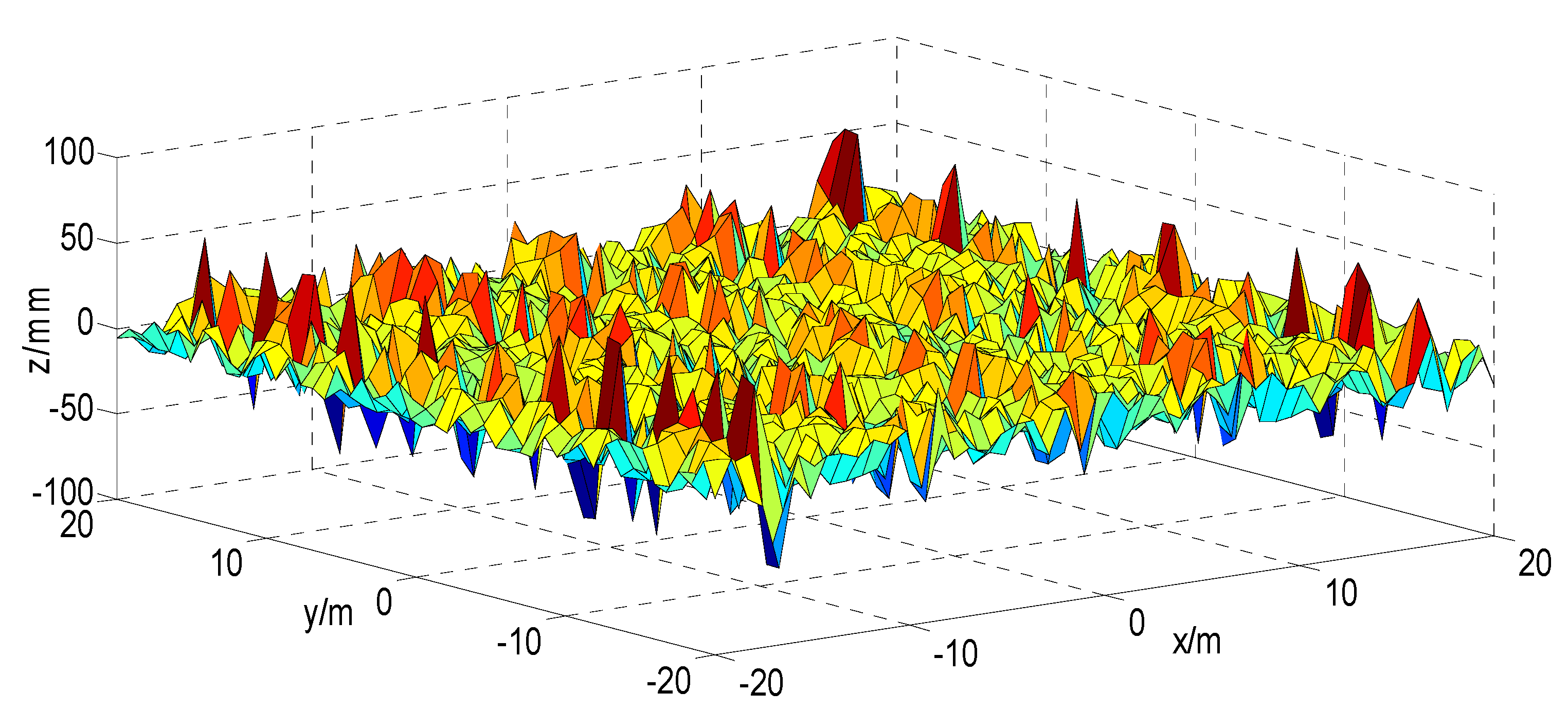
2.1. 3D Stochastic Road Surface Modeling Based on the Sine Wave Superposition Method

The unevenness of farmland ground requires real-time adjustment of the header height. In the spatial frequency domain, researchers generally study road surface roughness by studying road surface spectra. Similarly, road surface spectra can also be used to study the unevenness of farmland surfaces. System excitation arises from the irregularities in road elevation, serving as the primary excitation mechanism during vehicle operation. Numerous analytical tests demonstrate that road surface roughness exhibits characteristics of randomness, stationarity, and ergodicity. Road surface roughness can be analyzed and described through the theory of stationary stochastic processes. Some typical models include the harmonic superposition model, linear filtered white noise model, filtered Poisson model, and discrete time series model based on rational function PSD [16]. Here, a sine wave superposition model is employed to simulate variations in ground elevation. The fitting expression for the power spectral density G_q(n) of road roughness within the spatial frequency range n₁ < n < n₂ is as follows [17]:

$$G_q(n)=G_q(n_0){\left({\displaystyle \frac{n}{n_0}}\right)}^{-W}$$

(1)

In Equation (1), n₀ is the reference spatial frequency and the value is 0.1 m⁻¹; W is the frequency index of road power spectral density frequency structure, and the value is 2.

The variance of overall road surface roughness ${\sigma }_q^2$ can be expressed as follows:

$${\sigma }_q^2={\displaystyle {\int }_{n_1}^{n_2}{G}_q(n)d}n$$

(2)

For the convenience of computer processing, the spatial frequency range n₁ < n < n₂ is divided into m small intervals, the width of each small interval is $\Delta n_i$, and the value of the power spectral density of the pavement unevenness at the center frequency of each sub-interval $n_{mid,i}$ is substituted for the value in the range of sub-intervals $G_q\left(n_{mid,i}\right)$. Then, Equation (2) can be rewritten via discretization as follows:

$${\sigma }_q^2={\displaystyle \sum _{i=1}^m{G}_q(n_{mid,i})}\Delta n_i$$

(3)

By superimposing the sine wave functions between different communities, a two-dimensional random road roughness model is obtained:

$$q(x)={\displaystyle \sum _{i=1}^m{q}_i(x)}={\displaystyle \sum _{i=1}^m\sqrt{2G_q(n_{mid,i})\Delta n_i}\sin (2\pi n_{mid,i}x+{\theta }_i)}$$

(4)

Due to the random ergodicity of road surface roughness, it can be extended to another dimension, and the three-dimensional spatial road surface roughness can be expressed as follows [18]:

$$q(x,y)={\displaystyle \sum _{i=1}^m\sqrt{2G_q(n_{mid,i})\Delta n_i}\sin (2\pi n_{mid,i}x+{\theta }_i(x,y))}$$

(5)

Using MATLAB (R2013b) software to generate the spatial distribution of road surface roughness under given conditions, the results are shown in Figure 1. The generated result is a D-level road surface, with an x-axis length of 40 m and a y-axis length of 40 m, where $G_q(n_0)=1024\times {10}^{-6}$; the lower limit of spatial frequency n₁ is 0.008 m⁻¹; the upper limit of spatial frequency n₂ is 4.83 m⁻¹; and the iteration count m is set to 20.

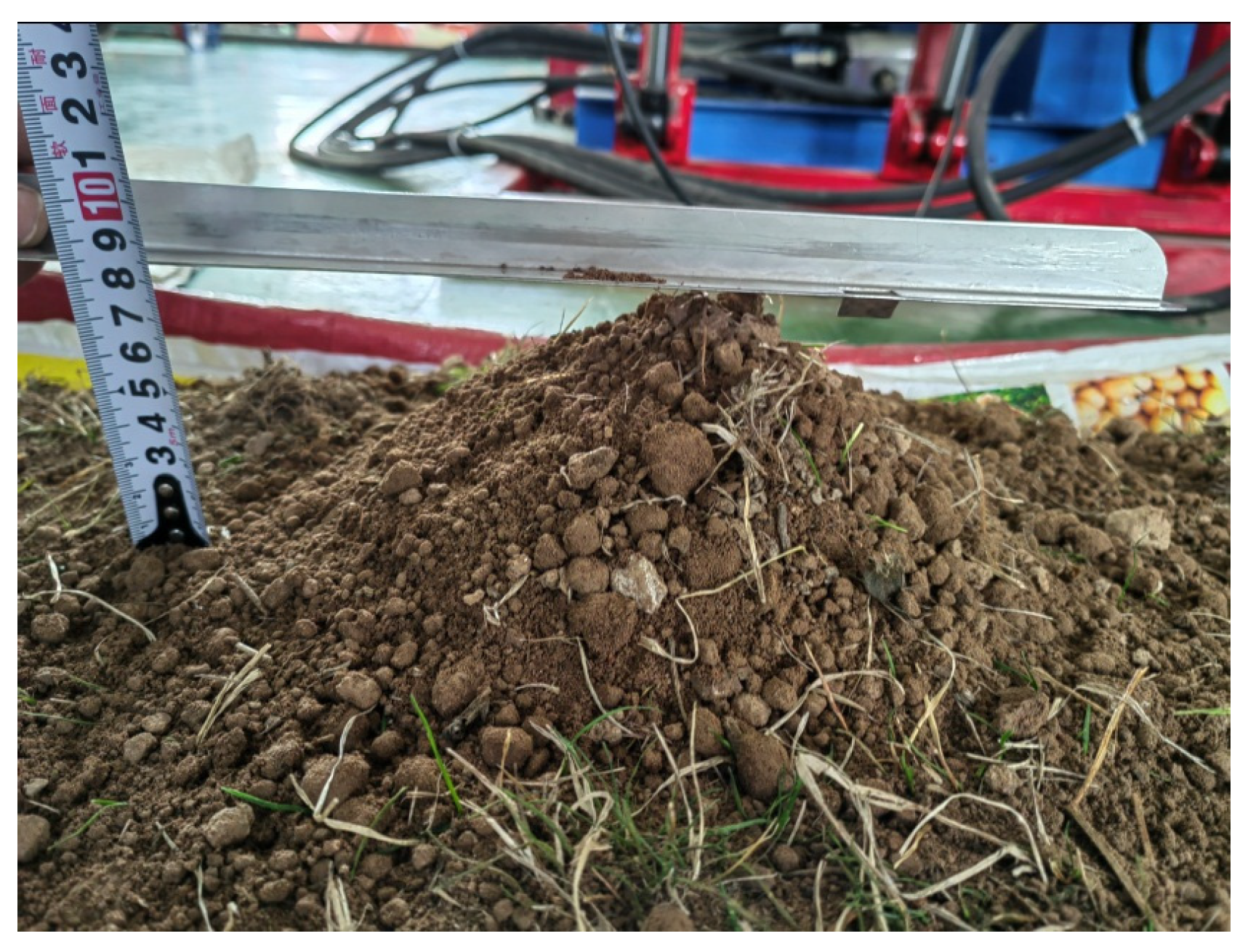
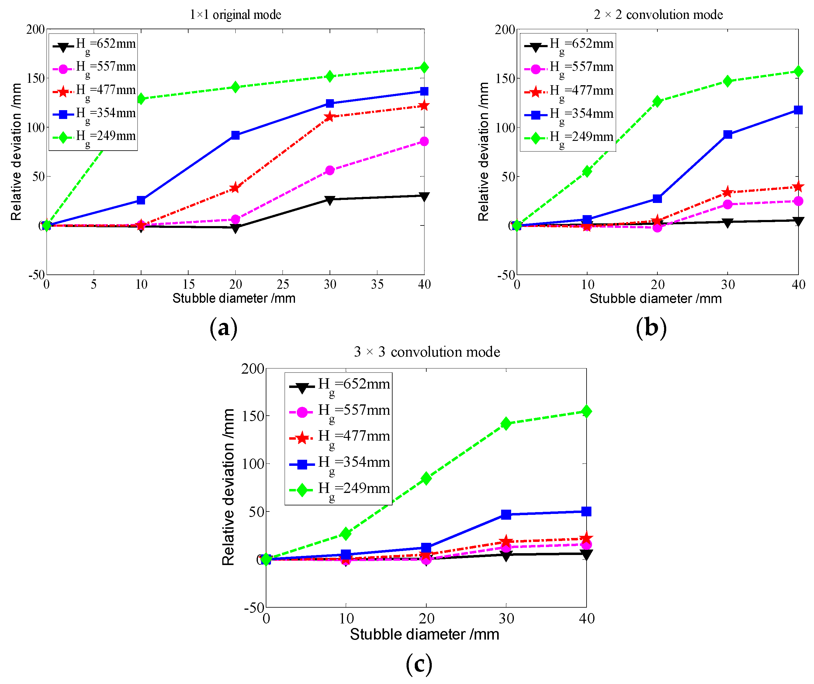
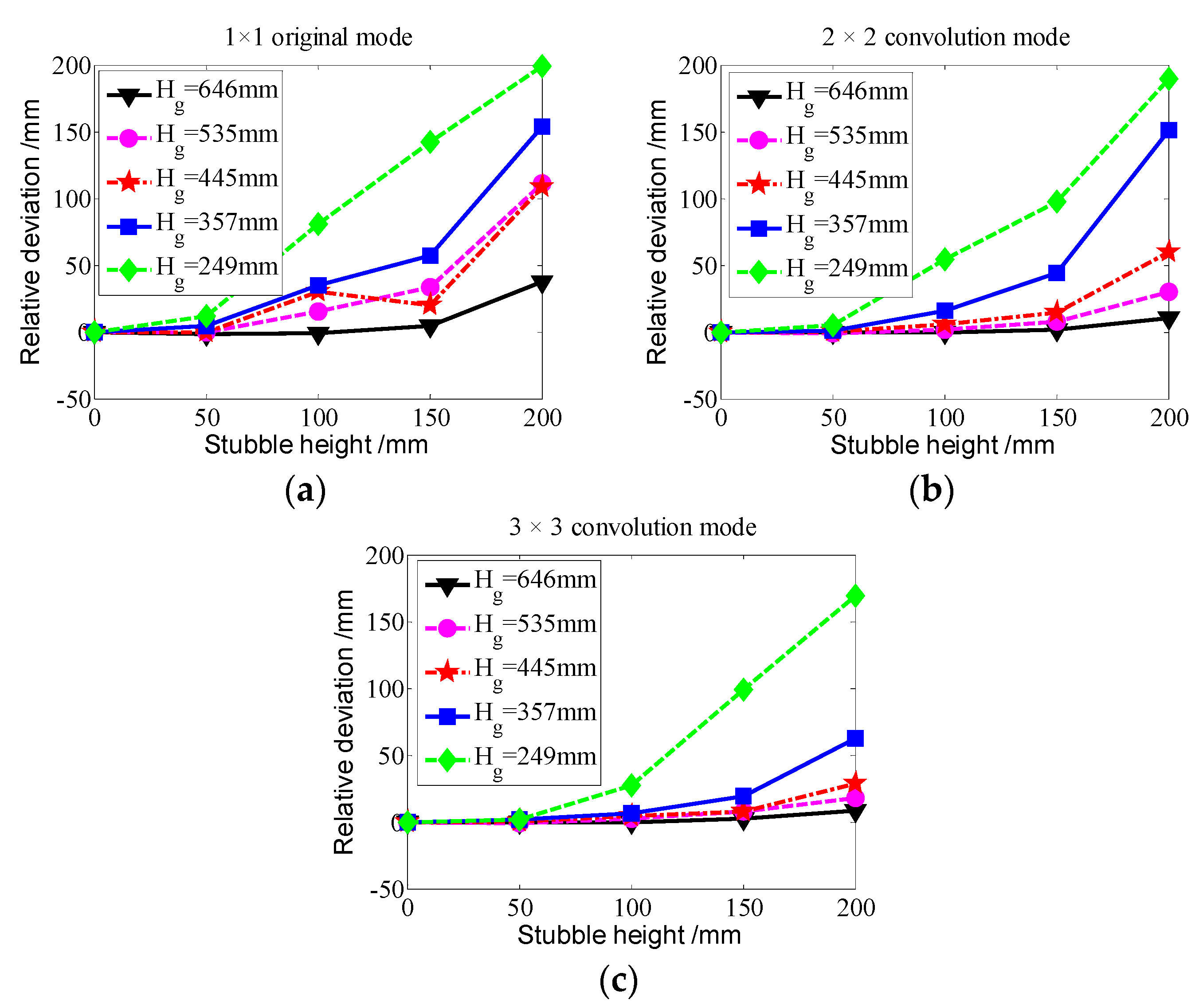
2.2. Data Acquisition and Analysis of the Area Array LiDAR

The TOFSense-M S array LiDAR produced by Nooploop Company (Shenzhen, China) was used to collect ground altitude data, with a ranging range of 1.5 cm~4 m and a distance resolution of 1 mm. The area array LiDAR can output 8 × 8 or 4 × 4 multi-point 3D cloud maps, based on UART communication mode, and the data communication format follows the NLink protocol. The diagonal field of view (FOV) angle is 63°, and both the horizontal and vertical directions are 45°. The FOV measurement area is a quasi quadriprism with a square bottom and a vertex in the emission window. The side length covering the square range on the measured plane is as follows:

$$R=L\times {\tan 45}^{\circ }$$

(6)

We selected the soil pile size, stubble diameter, and stubble height as the influencing factors of the sensor, and analyzed their impact on the measurement results. Figure 2 shows measurements of different soil pile heights, with a set angle of rest of 30 degrees and soil pile diameters of 100, 200, 300, and 400 mm, respectively. The corresponding soil pile heights are 28.9 mm, 57.7 mm, 86.6 mm, and 115.5 mm, respectively.

Figure 3 shows the measured effect of stubble on sensor measurement results. The stubble diameters were set to 10, 20, 30, and 40 mm, and the stubble heights were set to 50, 100, 150, and 200 mm. The measurements were taken at different ground heights.

The sensor 8 × 8 array data in the upper computer were exported using the query output method. Figure 4 shows a three-dimensional surface map with a stubble height of 150 mm converted into a ground perspective.

The spatial data were filtered using the 2 × 2 and 3 × 3 neighborhood averaging methods, respectively (where 1 × 1 represents the original data), and the minimum measurement value was selected as the statistical parameter. The measurement results with only ground were used as the reference value for calculation. The relative measurement errors under different factors such as stubble diameter, stubble height, and soil pile size were calculated. The impact of measurement results is shown in Figure 5, Figure 6, and Figure 7, respectively.

In Figure 5, it can be seen that when the height Hg of the sensor above the ground is fixed, the relative measurement value increases with the increase in the stubble diameter. This increase in the relative measurement value occurs because the equivalent area of the stubble diameter gradually increases, but the increase in the value is not significant when the height above the ground is high. Moreover, when the ground clearance was 652 mm, the diameter of the stubble increased from 0 to 40 mm, and the original measurement result increased by 30.35 mm. However, using the 2 × 2 and 3 × 3 modes, the neighborhood average rule increased by 4.85 mm and 5.72 mm, respectively. This indicates that the neighborhood averaging method can effectively weaken the influence of stubble diameter on the measured values.

In Figure 6, it can be seen that when the height Hg of the sensor above the ground is fixed, the relative measurement value also increases with the increase in the stubble height. This increase in the relative measurement value occurs because the equivalent area of the stubble height is gradually increasing, and the value increases slightly when the height above the ground is high. Moreover, when the ground clearance was 646 mm, the cutting height increased from 0 to 200 mm, and the measurement result only increased by 37.24 mm. However, using the 2 × 2 and 3 × 3 modes, the neighborhood average rule increased by 10.48 mm and 8.15 mm, respectively. This indicates that the neighborhood averaging method can effectively weaken the influence of stubble height on the measured values.

In Figure 7, it can be seen that when the height Hg of the sensor above the ground is fixed, the relative measurement value also increases as the size of the soil pile increases. This increase in the relative measurement value occurs because the equivalent area of the soil pile size is gradually increasing, and the effect of the height above the ground on the results is not very obvious. When the height above the ground is 249 mm and 652 mm, respectively, the diameter of the soil pile is selected as 400 mm, and the measurement results increase by 78.38 mm and 60.35 mm, respectively. However, using the 2 × 2 mode neighborhood average rule, the results increase by 78.38 mm and 59.52 mm, respectively. Moreover, using the 3 × 3 mode neighborhood average rule, the results increase by 78.6 mm and 54.01 mm, respectively. This indicates that the neighborhood averaging method effectively weakens the interference of stubble while detecting soil piles to the greatest extent possible.

2.3. Mathematical Model of Electromagnetic Directional Valve

Most existing harvesters use electromagnetic directional valves. Compared with hydraulic cylinder control systems with servo valves and proportional valves, hydraulic control systems based on electromagnetic directional valves have lower manufacturing and maintenance costs, higher reliability, and longer service life. However, due to their limited acceptance of discrete switch input signals with large switching delays, it is difficult to achieve precise positioning control [19]. This system uses a three-position four-way electromagnetic directional valve as the control element, model 4WE6J61B (Beijing, China). Its dynamic response is a coupled process of electro-generated magnetism, magnetic force, and force-generated motion. Its working principle can be described through circuit equations, magnetic circuit equations, and mechanical motion equations.

2.3.1. Circuit Equation

The driving circuit only energizes the electromagnetic coil during the opening and holding stages of the solenoid valve, without considering the influence of temperature on resistance and ignoring the additional resistance and inductance of the coil circuit. Therefore, the dynamic equation of the coil circuit during the opening and holding stages of the solenoid valve core is as follows [20]:

$$u=iR+L{\displaystyle \frac{di}{dt}}=iR+{\displaystyle \frac{d\psi }{dt}}=iR+N{\displaystyle \frac{d\varphi }{dt}}$$

(7)

In Equation (7), $u$ is the excitation voltage of the coil; i is the coil current; R is the coil resistance; and Φ is the magnetic flux of the electromagnetic system.

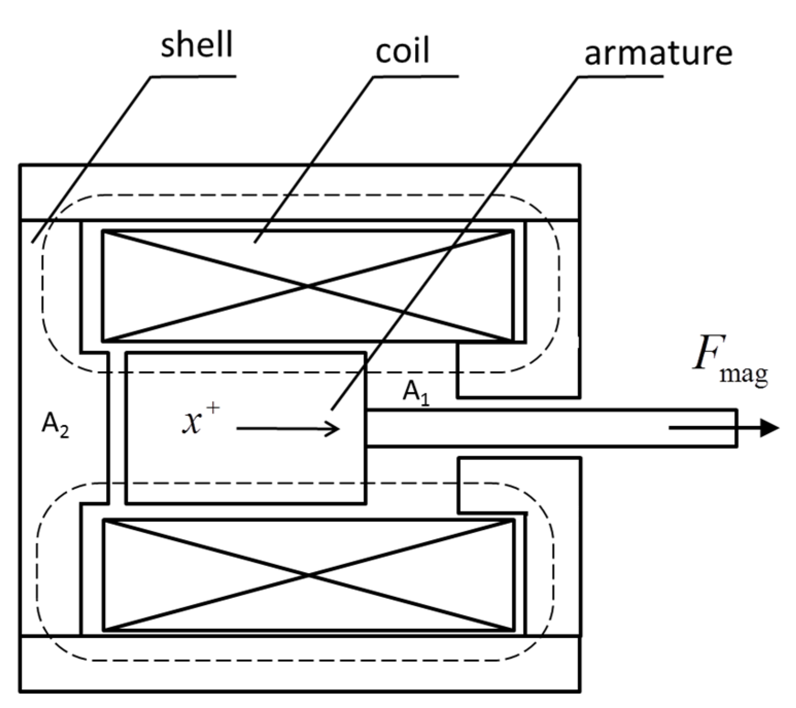
2.3.2. Magnetic Circuit Equation

The electromagnet is composed of a coil, an armature, and a shell, and its structural diagram is shown in Figure 8. The magnetic induction line of the main magnetic circuit after the electromagnetic coil is energized is indicated by the dashed line in Figure 8. Due to the small working air gap of the electromagnet, the magnetic circuit analysis method is used to calculate the parameters of the magnet. The magnetic permeability of the iron core and sleeve is much higher than that of air. Generally, the air gap magnetic resistance is tens of times that of a magnetic conductor; therefore, it can be approximated that the magnetic resistance of the magnetic path is mainly manifested in the air gap. That is, the magnetic energy of the system is concentrated in the air gap, and the magnetic conductor magnetic resistance can be ignored. Therefore, the magnetic circuit is mainly concentrated on the air gap magnetic resistance on the left and right sides, namely R_m1 and R_m2; the resistance values of the left and right sides are shown in Equation (8). The main magnetic circuit reluctance is equivalent to two magnetic resistances connected in series as follows [21]:

$$R_{m1}={\displaystyle \frac{S-x}{{\mu }_0{A}_1}}, R_{m2}={\displaystyle \frac{x}{{\mu }_0{A}_2}}$$

(8)

where μ₀ is the vacuum magnetic permeability, and the relationship between the coil inductance and magnetic resistance is as follows:

$$L={\displaystyle \frac{N^2}{R_{m1}+R_{m2}}}={\displaystyle \frac{{\mu }_0{A}_1{A}_2{N}^2}{A_{3}x+A_{2}S}}$$

(9)

where A₁ is the area of the outer ring air gap, A₂ is the area of the inner ring air gap, and A₃ = A₁ − A₂.

$$A_1={\displaystyle \frac{\pi }{4}}(D_1^2-d_1^2), A_2={\displaystyle \frac{\pi }{4}}{D}_1^2$$

(10)

According to the fundamental theorem of the Kirchhoff magnetic circuit, a mathematical model for magnetic circuit calculation can be obtained [22]:

$$Ni=\varphi R_m=\varphi ({\displaystyle \frac{s-x}{{\mu }_0{A}_1}}+{\displaystyle \frac{x}{{\mu }_0{A}_2}})$$

(11)

The electromagnetic force coefficient of the electromagnet $K_{emf}$ is as follows:

$$K_{emf}={\displaystyle \frac{dL}{dx}}=-{\displaystyle \frac{{\mu }_0{A}_1{A}_2{A}_3{N}^2}{{(A_{3}x+A_{2}S)}^2}}$$

(12)

The thrust magnitude of the electromagnet is as follows:

$$F_{mag}={\displaystyle \frac{1}{2}}{K}_{emf}{i}^2$$

(13)

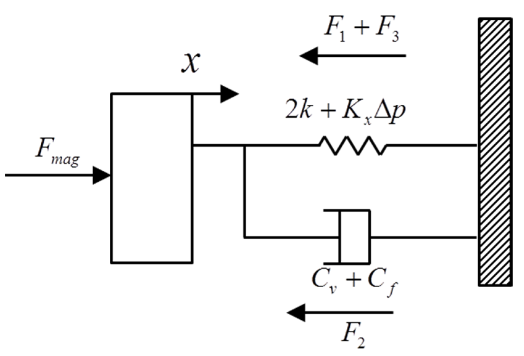
2.3.3. Mechanical Motion Equation

After the solenoid valve is energized, the coil is energized to generate electromagnetic attraction, which overcomes the spring force and friction, attracts the armature to push the push rod, and the valve core moves. The equivalent mechanical motion diagram is shown in Figure 9.

The motion equation of the valve core is as follows:

$$F_{mag}-F_1-F_2-F_3=m{\displaystyle \frac{d^{2}x}{d{t}^2}}$$

(14)

$$F_1=2kx, F_2=f_v+f=(C_v+C_f){\displaystyle \frac{dx}{dt}}, F_3=K_x\Delta p(x-d_0)$$

(15)

$$F_{mag}-(2k+K_x\Delta p)x-(C_v+C_f){\displaystyle \frac{dx}{dt}}+K_x\Delta p{d}_0=m{\displaystyle \frac{d^{2}x}{d{t}^2}}$$

(16)

where F₁ is the spring force, F₂ is the dynamic friction force between the valve core and valve body, as well as the hydraulic oil viscous damping force, and F₃ is the steady-state hydraulic force.

A dynamic process simulation model for the electromagnetic directional valve core was built based on Equations (7)–(16). The simulation model parameter settings are shown in

Table 1. Simulation parameters of electromagnetic directional valve.

Parameter	Symbol	Value	Parameter	Symbol	Value
Armature with rod end area	A1	56.67 mm2	Spring stiffness	k	4.6 N/mm
Armature without rod end area	A2	84.95 mm2	Cover length	d0	1 mm
Electromagnetic stroke	S	3 mm	Hydrodynamic coefficient	Kx	6.88 × 10−4
Permeability of vacuum	${\mu }_0$	4π × 10−7	Speed damping coefficient	Cv	0.005 Pa·s
Turns	N	3000	Oil viscosity damping coefficient	Cf	0.005 Pa·s
Coil resistance	R	6 Ω	Valve core quality	m	50 g
Excitation voltage	U	12 V/0 V	Pressure drop	∆p	6.85 Mpa

. The simulation duration was set to 0.2 s. The variation in excitation voltage and valve core displacement over time when the solenoid valve is powered on for 0.05 s and held for 0.1 s before disconnecting is shown in Figure 10.

As shown in Figure 10, the valve core begins to move at 50 ms and reaches a 3 mm travel point at 93.93 ms, with a connection time of 43.9 ms. When the excitation voltage jumps from 12 V to 0 V in 0.15 s, the electromagnet loses power, but the initial electromagnetic force is still large, and the valve core remains stationary. At 167.8 ms, the valve core begins to retreat, and at 171.3 ms, it returns to the origin position. Therefore, the valve disconnection time is about 21.3 ms. According to the technical manual, the opening time of this model of solenoid valve is 20–45 ms, and the closing time is 10–25 ms. Therefore, the simulation results are within the scope of the manual, proving the correctness of the simulation.

2.3.4. Analysis of Hydraulic System Control Strategy

A physical model of the hydraulic system was constructed using the Simscape module in Simulink (R2013b), as shown in Figure 11. The main parameters of the hydraulic system are as follows: the pump displacement is 25 mL/r; the motor speed is 1460 r/min; the opening pressure of the relief valve is 10 Mpa; the total stroke of the hydraulic cylinder is 200 mm; the piston diameter is 40 mm; and the piston rod diameter is 22 mm. The cutting table is replaced by a parallelogram structure with a magnification of 5.

The input of the electromagnetic directional valve can be represented as a set, U = {U₊, U₀, U₋}, corresponding to the hydraulic cylinder rising, holding, and falling, respectively. The Bang Bang switch predictive control system with position threshold was introduced to achieve early switching of the electromagnetic directional valve circuit. The ground elevation was set to q(t), the cutting height was set to h₀(t), and the actual height was h (t). The cutting height error e is defined as h(t)-q(t). When |e| is less than the position setting value plus threshold ε, the electromagnetic directional valve does not operate. When e is greater than the position setting value plus threshold ε, it indicates that the ground elevation increases, the cutting position is lower, and the cutting table needs to rise. When e is less than the position setting value plus threshold −ε, this indicates that the ground elevation decreases, the cutting table position is higher, and the cutting table needs to descend. The expression for the control algorithm is as follows:

$$U=\left\{\begin{array}{c}{U}_{+}\\ U_0\\ U_{-}\end{array}\right.\begin{array}{c} \mathrm{e}>h_0(t)+\epsilon \\ \left|\mathrm{e}\right|<h_0(t)+\epsilon \\ \mathrm{e}<h_0(t)-\epsilon \end{array}$$

(17)

The initial value of the height of the cutting table h(t) is set to 0.2 m, and h₀(t) is set to 0.2 m. The position thresholds ε are set to 0.5 cm, 1 cm, and 2 cm, respectively. The ground elevation change is simulated using a step signal. The initial value is 0 m, and it jumps to 0.2 m at 1 s. The ground elevation and cutting table height change curves under different position thresholds are shown in Figure 12. As shown in the figure, when the threshold is 0.5 cm, due to the small lead, the electromagnetic directional valve constantly switches up and down, and the cutting table oscillates continuously and cannot balance. When the threshold is 1 cm, the final height of the cutting table after experiencing two oscillations is 0.3917 m. Moreover, when the threshold is 2 cm, the header has no overshoot and reaches a steady state at 2.011 s, with a height of 0.416 m.

Based on the sine wave superposition method, a D-level random road surface was established to analyze the cutting table height change. Ground elevation (random signal) and cutting height curve are shown in Figure 13. If the position threshold ε is selected as 2 cm, the hydraulic cylinder does not act within 0–1.19 s due to the ground elevation change not exceeding 2 cm. At 1.194 s, the ground elevation change reaches 2.089 cm, exceeding the threshold. At this time, the hydraulic cylinder is ready to rise. Due to the delay in the electromagnetic valve signal rise, the hydraulic cylinder only rises at 1.23 s and stops at 1.381 s. Overall, the results present a control effect of the hydraulic cylinder changing for large undulating road surfaces but not adjusting for small undulations.

3. Results and Discussion

3.1. Control System Design

A cutting table height automatic control system was developed based on the STM32 microcontroller, and its circuit diagram is shown in Figure 14. The USART2 communicates with the serial port screen, which can set h0 (t) and the position threshold ε, and display the current radar data, hydraulic cylinder displacement value, and control mode in real time. The USART3 is used to measure the real-time displacement of hydraulic cylinders. The hydraulic cylinder displacement sensor outputs 4–20 mA current signals corresponding to travel distances of 0–200 mm. The current is converted to a 485 module and Modbus RTU protocol is used for data communication with the microcontroller. The UART4 communicates with an area array LiDAR, and the protocol analysis example is based on the NLink protocol. The electromagnetic valve is driven by the Infineon high-power driver chip BTN7970 to form an H-bridge driver module, which has the function of overheating and overcurrent protection. Using the 74HC244 chip to effectively isolate the microcontroller from the electromagnetic valve drive, KEY1 is used to select automatic or manual mode.

3.2. Laboratory Performance Test Results and Analysis

The agricultural machinery hydraulic automatic control test bench independently developed by Shanxi Agricultural University was used for testing in the laboratory, and the test diagram is shown in Figure 15. In order to secure the sensor in the position offacing the ground without tilting when the height of the cutting table changes, we used a parallel four-bar mechanism to simulate the header. We employed a total of four parallel four-bar mechanisms, each of which is equipped with hydraulic cylinders of different specifications. The extension and contraction of the hydraulic cylinder drive the cutting table to rise and fall, with a range of 1 m. A soil groove with a width of 0.5 m and a length of 3 m was created at the bottom of the cutting table, with three obvious soil mounds arranged on top of the groove and directional wheels arranged under the groove. Next, we set h0 (t) to 20 cm, the threshold of the cutting table ε was set to 2 cm, and the forward speed of the cutting table was set to 0.3 m/s. A high-speed camera was used to collect videos of the soil pile and cutting table and conduct motion analysis. As shown in the results in Figure 16, before 1 s, the ground elevation changed between 1.47 cm and 2.27 cm. At this time, the height of the cutting table was 20.8 cm, which was within the threshold range, and the hydraulic cylinder did not move. At 1.2 s, the ground elevation increased to 3.41 cm and continued to increase, at which point the header began to rise at a speed of 0.23 m/s. The header remained essentially unchanged from 1.623 s to 2.801 s. From 2.801 s to 3.24 s, the cutting table began to descend at a speed of 0.21 m/s, and there was no overshoot during the process of raising or lowering the cutting table. According to GBT 5117-2006, ”Whole-feed combine harvester—Technical requirements” [23], the lifting speed of the header should not be less than 0.2 m/s, and the lowering speed should not be less than 0.15 m/s. According to the experimental data, the system response speed during the lifting process of the cutting table is higher than the national standard.

3.3. Discussion

Most of the existing cutting platform height detection systems adopt the “single point” measurement method, which means that the sensor only outputs one value at a certain time and there is relatively little research on multi-point elevation measurement in the two-dimensional surface plane. Due to the complex and variable terrain of farmland, local singular values are easily generated. Therefore, this study investigated the three-dimensional microterrain detection technology using area array LiDAR for multi-point detection of cutting height, which can provide a more accurate and comprehensive three-dimensional model of the surface contour for cutting height control. By selecting common environmental factors in the field, such as soil mounds and stubble, and analyzing the impact of different sizes on the measurement results of the area array LiDAR, the neighborhood averaging method was adopted to effectively weaken the interference of stubble while detecting the presence of soil mound terrain to the greatest extent possible. In addition, common control strategies include PID, LQR, and some modern control methods such as robust adaptive control and self-disturbance rejection control. Qian Wang proposed an intelligent control algorithm for cutting table profiling based on multi-sensor data fusion and model predictive control (MSD-MPC), which can achieve high-precision, stable, and reliable cutting table height control [24]. However, most MSD-MPC methods use proportional solenoid valves to control the lifting and lowering of hydraulic systems. Furthermore, although the control accuracy of MSD-MPC methods is high, the cost is also significant. Due to the undulating terrain of farmland harvesting, blindly pursuing complete parallelism with the ground requires frequent action of the hydraulic system, and long-term high-speed switching causes the valve body to be prone to fatigue failure, which results in defects in service life and reliability. Therefore, the control strategy of not adjusting for small undulating roads and only adjusting for large undulations is more reasonable. At the same time, using lower-cost electromagnetic directional valves is more practical. Therefore, within an acceptable range of accuracy, the system can be more reliable, with a longer service life and lower maintenance costs.

4. Conclusions

(1)

In response to the problem of automatic control of header height, this study simulated three-dimensional ground elevation fluctuations based on a sine wave superposition model, which can generate the spatial distribution of road roughness of different levels as needed.

(2)

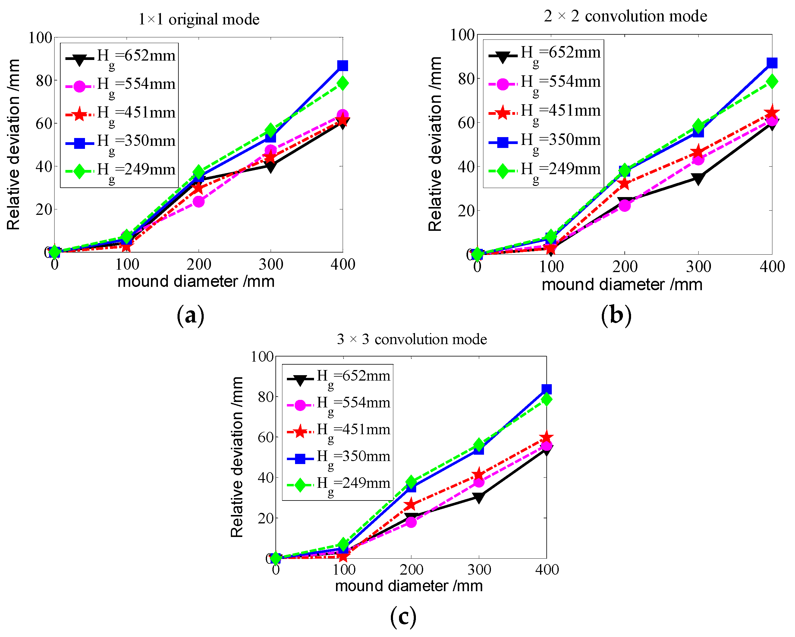
Using an area array LiDAR to collect data on a cutting height of 8 × 8, the influence of soil mounds and stubble on the measurement results was analyzed. The results showed that the neighborhood averaging method effectively weakened the interference of stubble while detecting soil mounds to the maximum extent possible.

(3)

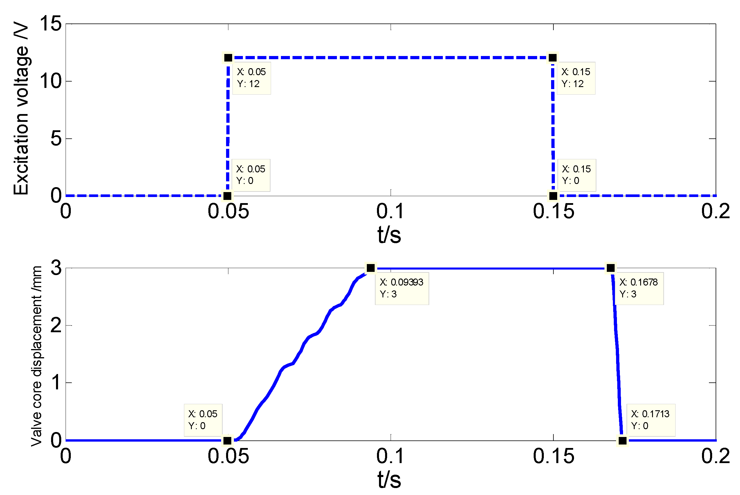
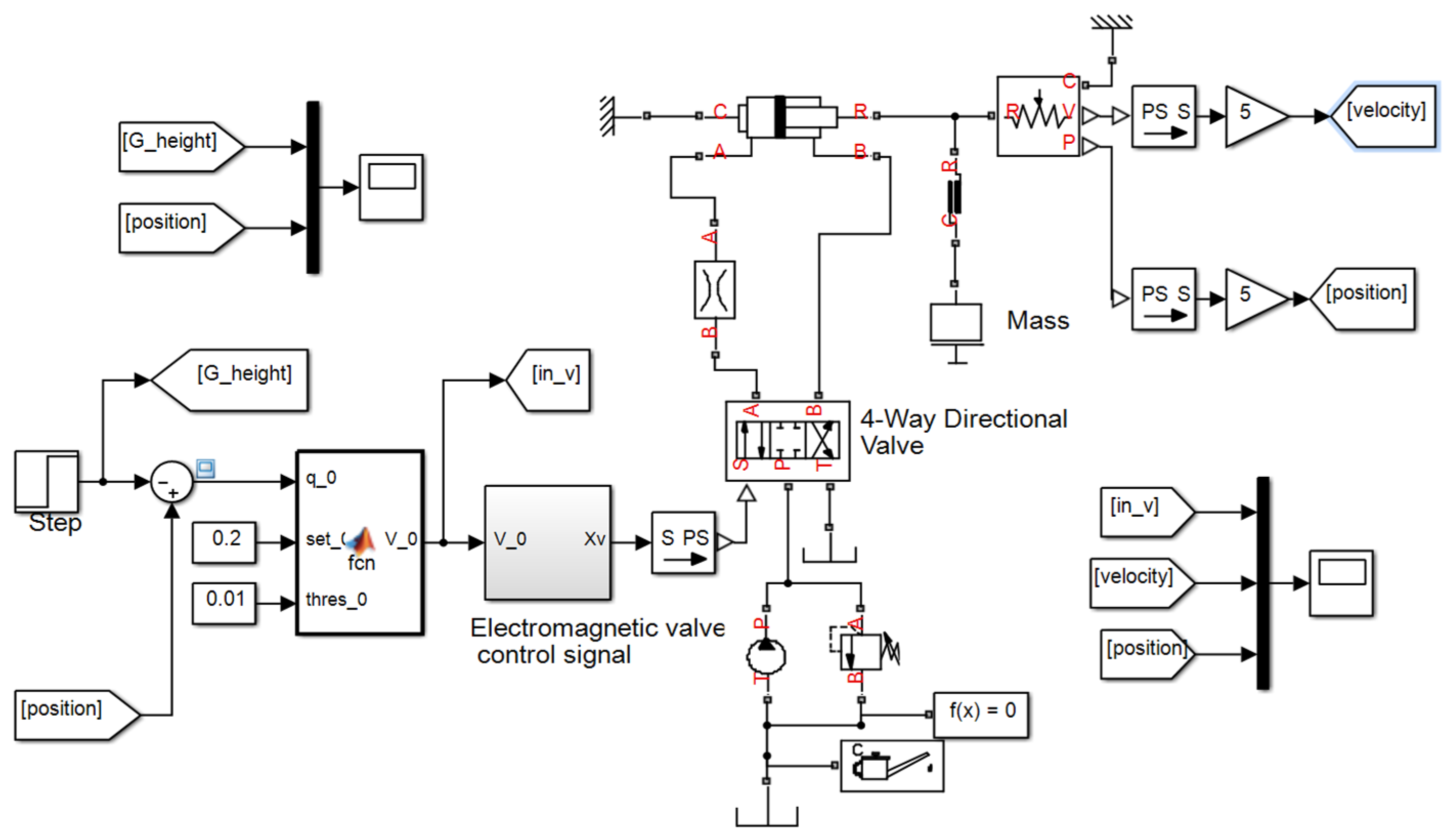
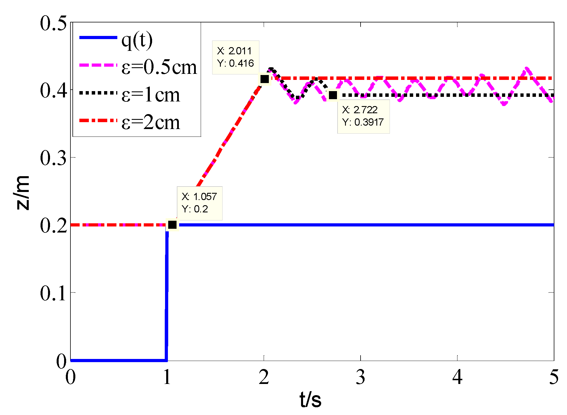
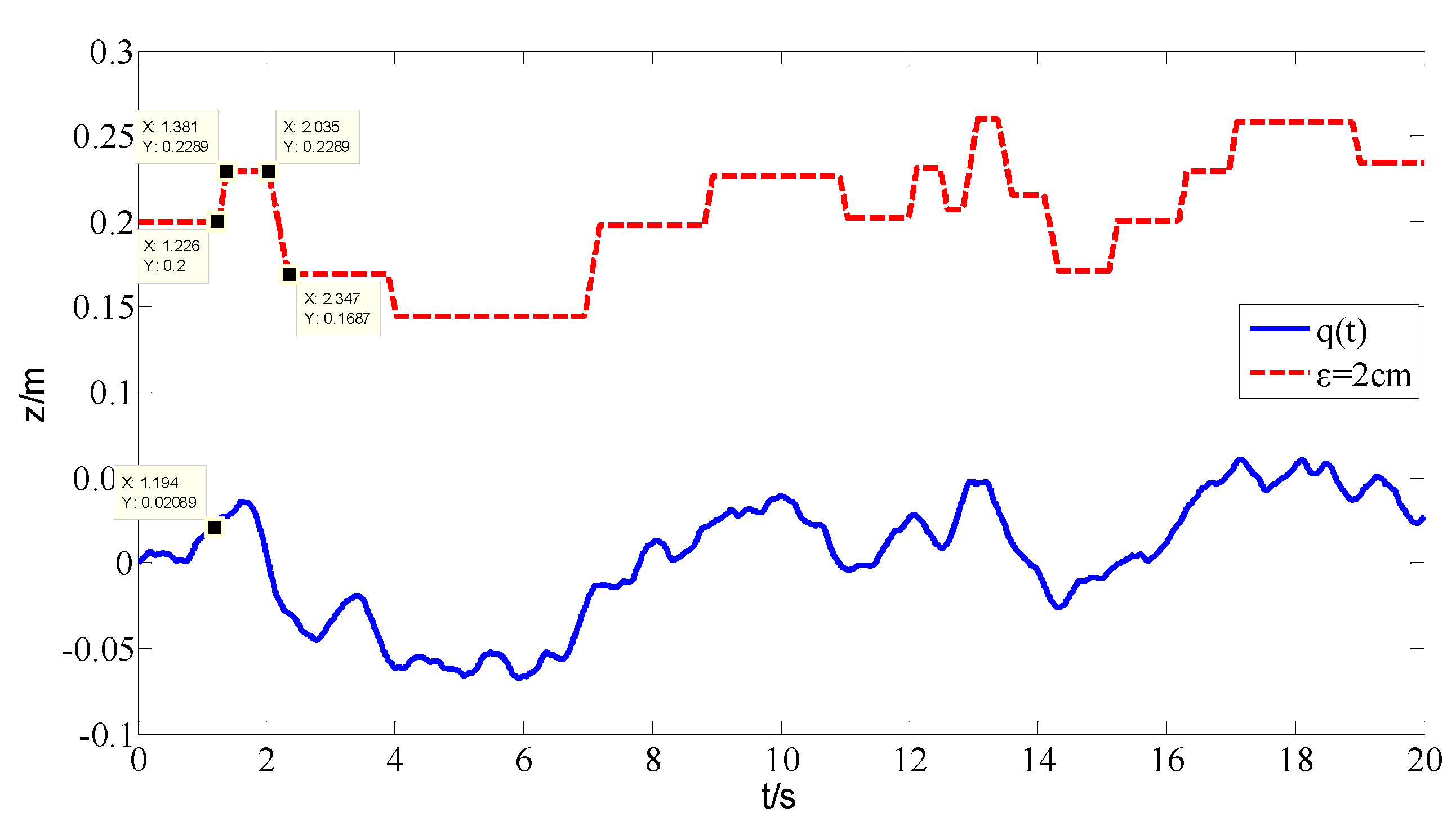
A dynamic process simulation model of the electromagnetic directional valve core was constructed, and the on/off delay characteristics of the electromagnetic directional valve were analyzed. Using the Simscape module in Simulink, a physical model of the hydraulic system was constructed, and the Bang Bang switch predictive control system with a position threshold was introduced to achieve early switching of the electromagnetic directional valve circuit. Then, the variation in the header height under different position thresholds was analyzed.

(4)

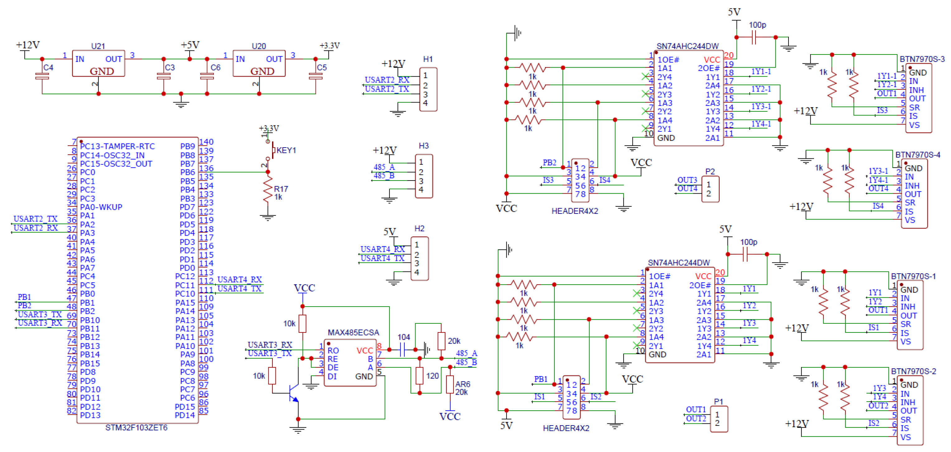
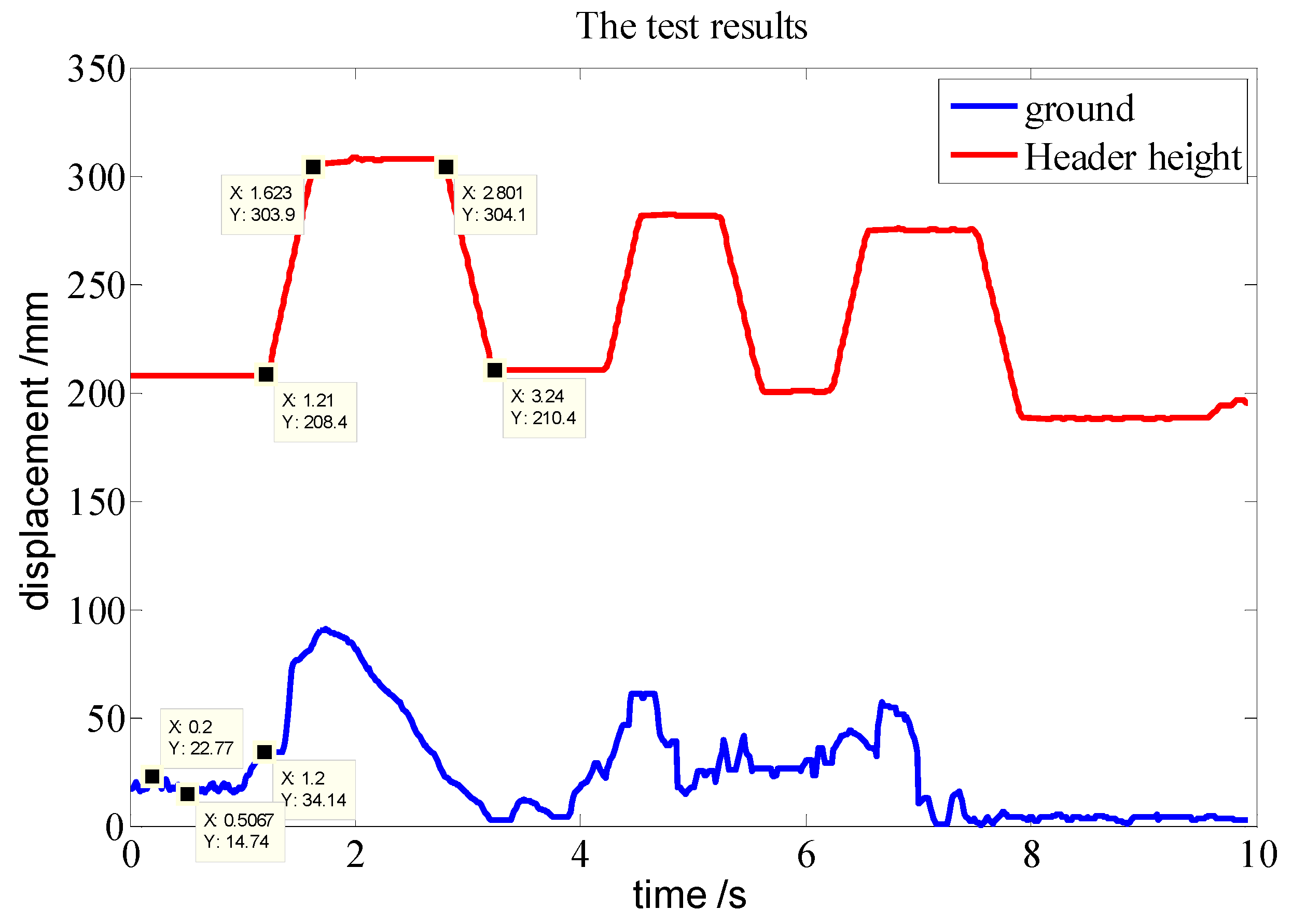
An automatic control system for the height of the cutting table was developed based on the STM32 microcontroller. Experimental tests were conducted using the agricultural machinery hydraulic automatic control test bench independently developed by Shanxi Agricultural University. Overall, the control effect showed that the hydraulic cylinder did not adjust in response to a small undulating road surface; the hydraulic cylinder only adjusted in response to a large undulating road surface. At the same time, there was no overshoot during the lifting process of the cutting table, with a rising speed of 0.23 m/s and a falling speed of 0.21 m/s. The system response speed was higher than the national standard; therefore, the proposed automatic control system meets practical usage requirements.

References

1. Pask, G.S.; Wilson, J.N.; Zoerb, G.C. Automatic Header-Height Control System for Windrowers. Trans. Asae 1974, 17, 597–602. [Google Scholar] [CrossRef]
2. Clayton, J.E.; Eiland, B.R. LaboratoryAnnual Report of the USDA Sugarcane Research; USDA Sugarcane Research Laboratory: Belle Glade, FL, USA, 1977; pp. 30–70. [Google Scholar]
3. Wright, M.E.; Simoneaux, J.J.; Drouin, B. Automatic height control of a sugarcane harvester basecutter. SAE Trans. 1998, 107, 239–246. [Google Scholar]
4. Neves, J.L.M.; Marchi, A.S.; Pizzinato, A.A.S.; Menegasso, L.R. Comparative testing of a floating and aconventional fixed base cutter. In Proceedings of the International Society of Sugar Cane Technologists, Brisbane, Australia, 17–21 September 2001; pp. 257–262. [Google Scholar]
5. Tulpule, P.; Kelkar, A. Integrated robust optimal design (IROD) of header height controlsystem for combine harvester. In Proceedings of the American Control Conference, Portland, OR, USA, 4–6 June 2014; pp. 2699–2704. [Google Scholar]
6. Geng, A.; Zhang, M.; Zhang, L.; Zhang, Z.; Gao, A.; Zheng, J. Design and Experiment of Automatic Control System for Corn Header Height. Trans. Chin. Soc. Agric. Mach. 2020, 51, 118–125. [Google Scholar]
7. Liu, Q.; Li, C.; Wei, X.; Lu, Z.; Wang, A. Research on the header height control strategy of combine harvester based on LQR. J. Electron. Meas. Instrum. 2022, 36, 65–72. [Google Scholar]
8. Guan, Y.; Jin, Z.; Bai, X.; Wang, S.; Wu, L.; Huang, W. Design and Experiment of Servo Control System for Sugarcane Header. Trans. Chin. Soc. Agric. Mach. 2023, 54, 119–128. [Google Scholar]
9. Liang, Z. Study on the Adaptive Control System of Sugarcane Harvester Based on Cutting Height Detection. Ph.D. Thesis, Chang’an University, Xi’an, China, 2022. [Google Scholar]
10. Suomi, P.; Oksanen, T. Automatic working depth control for seed drill using ISO 11783 remote control messages. Comput. Electron. Agric. 2015, 116, 30–35. [Google Scholar] [CrossRef]
11. Chang, K.Y.; Zaman, Q.; Farooque, A.; Rehman, T.; Esau, T. An on-the-go ultrasonic plant height measurement system (UPHMS II) in the wild blueberry cropping system. In Proceedings of the 2016 ASABE Annual International Meeting, Orlando, FL, USA, 17–20 July 2016. [Google Scholar]
12. Cleodolphi, D.; Verstraete, J.; Fagundes, A.; Sarchi, R.; Tanaka, F. Control of Base Cutter Height for Multiple Row Sugarcane Harvesters. America US09781880, 10 October 2017. [Google Scholar]
13. Chong, Z. Research on header profiling and crop height measurement method. Master’s Thesis, Southeast University, Dhaka, Bangladesh, 2020. [Google Scholar]
14. Huang, M. Research on Techniques of Wide and Multilayer Cutting and Its Adaptive Control for Ratoon Rice Harvesting. Ph.D. Thesis, Jiangsu University, Zhenjiang, China, 2021. [Google Scholar]
15. Liu, G.; Xia, J.; Zheng, K.; Cheng, J.; Wang, K.; Liu, Z.; Wei, Y.; Xie, D. Measurement and evaluation method of farmland microtopography feature information based on 3D LiDAR and inertial measurement unit. Soil Tillage Res. 2024, 236, 105921. [Google Scholar] [CrossRef]
16. Christlieb, A.; Lawlor, D.; Wang, Y. A multiscale sub-linear time Fourier algorithm for noisy data. Appl. Comput. Harmon. Anal. 2016, 40, 553–574. [Google Scholar] [CrossRef]
17. Li, J.; Zhang, Z.; Gao, X.; Wang, P.; Li, J. Relation between Power Spectral Density of Road Roughness and International Roughness Index and Its Application. Int. J. Veh. Des. 2019, 77, 247–271. [Google Scholar] [CrossRef]
18. Gardulski, J.; Adamczyk, J.; Targosz, J. Determination of the Stochastic Kinematic Excitation of the Car by the Real Profile of the Road Surface. Arch. Transp. 2011, 23, 447–454. [Google Scholar] [CrossRef]
19. Hou, T.; Kou, Z.; Wu, J.; Jin, T.; Su, K.; Du, B. Research on Positioning Control Strategy for a Hydraulic Support Pushing System Based on Iterative Learning. Actuators 2023, 12, 306. [Google Scholar] [CrossRef]
20. Jin, L. Study on the Precise Positioning Control of Hydraulic Cylinder Using Solenoid Operated Directional Control Valve. Ph.D. Thesis, Zhejiang University, Hangzhou, China, 2019. [Google Scholar]
21. Xu, J.; Wu, J.; Feng, S.; Zhou, Y. Reluctance analysis of rotary valve structure variable inductor. J. Magn. Mater. Devices 2018, 49, 39–43+68. [Google Scholar]
22. Rostami, M.; Naderi, P.; Shiri, A. Modeling and analysis of variable reluctance resolver using magnetic equivalent circuit. COMPEL Int. J. Comput. Math. Electr. Electron. Eng. 2021, 40, 921–939. [Google Scholar] [CrossRef]
23. Wei, L.; Dai, F.; Han, Z.; Li, X.; Gao, A. Experiment on plot wheat breeding combine harvester. Acta Agric. Zhejiangensis 2016, 28, 1082–1088. [Google Scholar]
24. Wang, Q.; Meng, Z.J.; Wen, C.K.; Qin, W.C.; Wang, F.; Zhang, A.Q.; Zhao, C.J.; Yin, Y.X. Grain combine harvester header profiling control system development and testing. Comput. Electron. Agric. 2024, 223, 109082. [Google Scholar] [CrossRef]
Figure 1. Three−dimensional randomized pavement unevenness distribution map.
Agriculture 14 01293 g001
Figure 2. Height measurement diagram of soil pile.
Agriculture 14 01293 g002
Figure 3. The measured effect of stubble on sensor measurement results.
Agriculture 14 01293 g003
Figure 4. Three−dimensional curved surface with a stubble height of 150 mm (ground perspective).
Agriculture 14 01293 g004
Figure 5. Analysis diagram of the impact of stubble diameter on the measurement results (stubble height: 100 mm). (a) 1×1 original mode; (b) 2 × 2 convolution mode; (c) 3 × 3 convolution mode.
Agriculture 14 01293 g005
Figure 6. Analysis of the impact of stubble height on the measurement results (stubble diameter: 25 mm). (a) 1 × 1 original mode; (b) 2 × 2 convolution mode; (c) 3 × 3 convolution mode.
Agriculture 14 01293 g006
Figure 7. Analysis of the impact of soil pile size on the measurement results (angle of rest: 30 degrees). (a) 1 × 1 original mode; (b) 2 × 2 convolution mode; (c) 3 × 3 convolution mode.
Agriculture 14 01293 g007
Figure 8. Structural diagram of the electromagnet.
Agriculture 14 01293 g008
Figure 9. Mechanical motion diagram of the solenoid valve core.
Agriculture 14 01293 g009
Figure 10. Simulation state curve of electromagnetic directional valve opening and closing characteristics.
Agriculture 14 01293 g010
Figure 11. Physical model of the hydraulic system constructedusing the Simscape module.
Agriculture 14 01293 g011
Figure 12. Ground elevation (step signal) and header height curve under different position thresholds.
Agriculture 14 01293 g012
Figure 13. Ground elevation (random signal) and cutting height curve.
Agriculture 14 01293 g013
Figure 14. Circuit diagram of an automatic control system for cutting height based on the STM32 microcontroller.
Agriculture 14 01293 g014
Figure 15. Experimental testing of hydraulic automatic control test bench for agricultural machinery.
Agriculture 14 01293 g015
Figure 16. Experimental testing curve for ground elevation and cutting table height.
Agriculture 14 01293 g016