Vegetable Commodity Organ Quality Formation Simulation Model (VQSM) in Solar Greenhouses

Abstract

Cucumber (Cucumis sativus L.) and celery (Apium graveolens L.) are among the most widely cultivated vegetable crops, belonging to the melon and leafy vegetable categories, respectively. This study aims to provide predictions for the quality formation of greenhouse cucumber and celery, as well as technical support for intelligent vegetable production management. Based on the light and temperature response characteristics of cucumber and celery growth and development and using the experimental varieties ‘Jinsheng 206’ for cucumber and ‘Juventus’ for celery, the observational data from a five-cropping season trial over 2 years were utilized. By analyzing the relationship between the growth and development of vegetables and key meteorological factors (radiation and temperature), simulation models for quality formation were constructed using the day–night temperature difference method (ATD) and the product of thermal effectiveness and the photosynthetically active method (TEP) as independent variables. The model parameters were determined and the model was validated using independent trial data. The results showed the following: (1) There exist quantifiable relationships between different quality indicators and ATD or TEP. These relationships are mainly presented through linear functions, exponential functions, logarithmic function, and logical functions. (2) The normalized root mean square error (NRMSE) of the cucumber quality model ranges from 1.13% to 29.53%, and the NRMSE of the celery quality model ranges from 1.63% to 31.47%. (3) Based on two kinds of normalization methods, the average NRMSE of the VQSM model is 13.72%, demonstrating a relatively high level of accuracy in simulation. These results demonstrate that the proposed model can dynamically and accurately simulate the quality formation process of vegetables, providing a theoretical basis and data support for the research on productivity and the economic benefits of greenhouse crops.

1. Introduction

As of 2020, the total area of facility cultivation in China exceeded 4 million hectares. The area of facility vegetable cultivation continues to expand, with nearly 40% of vegetables being provided by solar greenhouses. Among them, the supply rate of facility-grown vegetables in autumn and winter exceeds 90% [1]. Cucumber (Cucumis sativus L.) and celery (Apium graveolens L.) are among the most widely cultivated facility-grown melon and leafy vegetables globally [2,3]. Crop models are quantitative simulation models driven by environmental variables. They utilize computer technology and physical–mathematical methods to describe and predict the growth, development, and yield formation process of crops [4,5]. They are a mechanistic and numerical simulation model that can be applied to climate impact assessment [6], regional productivity prediction analysis [7], and digital design and decision support [8]. With the development of the vegetable industry and the increasing consumption levels of the population, the market not only focuses on vegetable yield, but also demands higher standards for vegetable quality [9,10]. Therefore, there is an urgent need to construct a dynamic simulation model for the formation of quality indicators in facility vegetable production, in order to achieve accurate quality prediction.

Vegetable quality refers to the external appearance and physicochemical properties of vegetable organs [9,11], which are mainly influenced by crop genetic factors [12] and environmental conditions such as temperature [13,14], light [14], and water and nutrient supply [15,16]. Scholars have developed vegetable productivity simulation models such as TOMGRO [17] and TOMSIM [18], which can quantify processes such as vegetable growth stages and phenological phases, organ development and establishment, photosynthetic production, substance accumulation, assimilate distribution, and yield quality formation. Studies have also been conducted on model uncertainty analysis [19], model coupling prediction analysis [20], and parameter sensitivity analysis [21]. However, these models have poor extrapolation ability, complex and diverse parameters that are difficult to obtain, and require a large amount of experimental data for parameter localization. Additionally, these models mainly focus on phenotypic characteristics and pay less attention to the changes in physicochemical quality. Therefore, there is an urgent need for a simulated model of vegetable quality formation with simple input data types and easily accessible variety parameters.

Under the reorganization of water and fertilizer management conditions, the external environmental factors that affect crop quality formation mainly include temperature and light. Research has shown that during the days with higher temperatures, plants undergo photosynthesis and accumulate sugars. During the cooler nighttime temperatures, the respiratory functions of plants are weakened, reducing sugar consumption, which affects fruit sweetness and flavor [22]. Diurnal temperature differences help promote the synthesis and accumulation of anthocyanins, carotenoids, and cell wall substances, which affect fruit color and firmness [23,24]. The larger the diurnal temperature difference, the more soluble sugars, sucrose, and soluble proteins accumulate in the fruit [25]. Positive diurnal temperature differences increase soluble sugars, the sugar-to-acid ratio, soluble proteins, and the vitamin C content, while decreasing the organic acid content. Conversely, negative diurnal temperature differences show the opposite trend [22]. The cumulative temperature–humidity index theory comprehensively considers the impact of temperature and light on crop growth and development by multiplying the thermal effect of temperature by the photosynthetically effective radiation. This index has been widely used to simulate yield and quality formation in horticultural crops such as celery [26], tomato [27,28], tulip [29], and tea [29], with high simulation accuracy. Most of the studies in this area have focused on the sensitivity of phenotypic traits to environmental factors. However, further exploration can be conducted to assess the applicability of these traits in determining the physiological and chemical quality indicators of vegetables. In terms of model evaluation, data normalization transforms data into specific ranges or distributions for subsequent data analysis and model training, which are commonly used in machine learning to scale data proportionally to fit within a specific range [30,31]. While most model research has been limited to the evaluation of specific indicators [26,29], there is potential to explore the use of normalization methods in model evaluation, aiming to provide a comprehensive assessment of the overall simulation performance.

Therefore, constructing a simulation model of vegetable crop quality formation based on the diurnal temperature difference and the heat accumulation algorithm has significant implications for vegetable production. This study quantifies the relationship between vegetable quality indicators and light–temperature environmental factors (diurnal temperature difference and heat accumulation) using temperature and radiation as the main driving variables. It compares and selects the optimal development modeling method for simulating the formation of vegetable crop quality in a greenhouse, determines the model’s parameters, and uses different normalization methods to comprehensively evaluate the simulation effect of the model. We can simulate the formation process of vegetable quality under the same cultivation environment conditions by inputting simple temperature radiation data, aiming to evaluate the differences in vegetable quality production potential under different climate change patterns. In addition, this study will provide technical support for intelligent vegetable production management and improve economic benefits.

2. Materials and Methods

2.1. Experimental Design

The experiment was carried out in the agricultural technology innovation base in Wuqing District, Tianjin City, China (longitude: 116.97° E, latitude: 39.43° N, elevation: 8 m), from 2018 to 2020. Cheng et al., 2024 introduced the parameters of greenhouse structure and soil physical and chemical properties [32]. The cucumber variety tested was ‘Jinsheng 206’ [32], and the celery variety tested was ‘Juventus’ [26]. The sowing dates and the number of days for key development stages were set as shown in

Table 1. Experimental period setting for stubble sowing and key development period days. The 9 groups with * were used in the model establishment, and the other 5 groups were used for model validation. AW refers to autumn–winter cultivation, while SC refers to spring cultivation.

Cucumber	Start Date/Y-M-D	End Date/Y-M-D	Celery	Start Date/Y-M-D	End Date/Y-M-D
AW in 2018	2018-09-20	2019-02-28	AW in 2018	2018-09-10	2019-03-14
	2018-10-17 *	2019-02-28		——	——
	2018-11-11	2019-02-28		2018-10-10 *	2019-03-14
SC in 2019	2019-03-10	2019-07-24	AW in 2019	2019-09-10	2020-04-14
	2019-03-26 *	2019-07-24		2019-09-24 *	2020-04-14
	2019-04-10	2019-07-24		2019-10-09	2020-04-14
AW in 2019	2019-09-20	2020-03-28
	2019-10-10 *	2020-04-05
	2019-11-01	2020-04-19

, with 3 replicates for each planting date. A randomized complete block design was used. The cucumber planting row spacing was 0.67 m, and the plant spacing was 0.42 m, resulting in a plot area of 16 m² and a planting density of 35,550 plants/ha. The celery planting row spacing was 0.38 m, and the plant spacing was 0.08 m, resulting in a plot area of 3.0 m² and a planting density of 321,400 plants/ha.

2.2. Data Sources

2.2.1. Crop Data

The firmness (F) of the commodity organ was determined using the GY-4 hardness tester. The commodity organ was tested at 2–3 cm from the bottom, middle, and top [33]. Each experiment was repeated 3 times to obtain the average value, and the data were recorded and processed. The firmness of cucumber fruit is recorded as $F_{friut}$, and the firmness of celery stem is recorded as $F_{stem}$.

To measure the average Lab color model values on the surface of each commodity organ, 3 points were selected on each commodity organ in random locations. Each point was measured 3 times using the 3nh NR110 precision colorimeter. The L*a*b color model consists of the L axis, representing brightness (ranging from 0 for black to 100 for white), the a axis, representing red (positive values) and green (negative values), and the b axis, representing yellow (positive values) and blue (negative values). The hue (H) is computed using Equation (1). The color value (CV) is computed using Equation (2) [34], and the darker value (DV) is determined using Equation (3) [35]. The colors of cucumber fruits are recorded as ${CV}_{friut}$, $H_{friut}$, and ${DV}_{friut}$, the colors of celery stems are recorded as ${CV}_{stem}$, $H_{stem}$, and ${DV}_{stem}$, and the colors of celery leaves are recorded as ${CV}_{leaf}$, $H_{leaf}$, and ${DV}_{leaf}$.

$$\mathrm{H}=\mathrm{b}/\mathrm{a}$$

(1)

$$\mathrm{C}\mathrm{V}=2000\times \mathrm{a}\times \sqrt{{\mathrm{a}}^2+{\mathrm{b}}^2}/\mathrm{L}$$

(2)

$$\mathrm{D}\mathrm{V}=100-\mathrm{L}$$

(3)

The appearance of the fruit was measured by using a ruler to measure the length ($L_{friut}$) and radian ($R_{friut}$) in centimeters and a PD-151 sliding caliper to measure the diameter ($D_{friut}$) in millimeters. Due to the fact that cucumber fruits exhibit a certain degree of radian ($R_{friut}$) during the actual production and harvesting process, we assume that cucumbers are curved cylinders and symmetrical, so the shape index of the fruit (SI) is the ratio of fruit length to fruit diameter, determined using Equation (4).

$${SI}_{friut}={\displaystyle \frac{2\times \sqrt[2]{{(L_{friut}/2)}^2+{R_{friut}}^2}}{D_{friut}/10}}$$

(4)

The number of celery stems ($N_{stem}$) and fully expanded leaves ($N_{leaf}$) was recorded. The leaf area (LA) of celery was measured using the coordinate paper method. The plant height ($H_{plant}$) of celery was measured using a ruler to determine the distance from the top of the plant’s root base to the plant’s tip.

According to Equation (5), the water content of the commodity organ is calculated based on the ratio of water content to fresh weight. The water content of the cucumber fruit is denoted as ${WC}_{fruit}$, while the water content of the celery main stem, leaf, and aboveground part are denoted as ${WC}_{stem}$, ${WC}_{leaf}$, and ${WC}_{overground}$, respectively.

$$\mathrm{W}\mathrm{C}=({\mathrm{W}}_{\mathrm{f}}-{\mathrm{W}}_{\mathrm{d}})/{\mathrm{W}}_{\mathrm{f}}\times 100\mathrm{\%}$$

(5)

where ${\mathrm{W}}_{\mathrm{f}}$ represents the fresh weight of the commodity organ (g), and the fresh weight of the celery main stem, leaf, and aboveground part are denoted as $W_{stem}$, $W_{leaf}$, and $W_{overground}$, respectively. ${\mathrm{W}}_{\mathrm{d}}$ represents the dry mass of the commodity organ (g). ${\mathrm{W}}_{\mathrm{d}}$ refers to each organ, which was divided into kraft paper bags and placed in an oven, g [32].

After washing and drying the yield organs, extract the juice. Measure the soluble solid content (SSC, Brix%) of the yield organ solution using a PAL-1 digital refractometer. Repeat the SSC measurement 3 times for each sample, and take the average of the repeated measurements as the final result. The SSC of cucumber fruit is recorded as (${SSC}_{fruit}$), and the SSC of the celery main stem, leaf, and aboveground parts are recorded as ${SSC}_{stem}$, ${SSC}_{leaf}$, and ${SSC}_{overground}$, respectively.

The cucumber soluble protein content (${SP}_{fruit}$) was determined using the Coomassie Brilliant Blue method (mg/g) [36]. The cucumber soluble sugar content (${SS}_{fruit}$) was measured using the Anthrone Colorimetric method (mg/g) [37]. The determination of vitamin C in cucumber fruit (${VC}_{fruit}$) was carried out using the 2,4-dinitrophenylhydrazine method (mg/kg) [38].

To measure the chlorophyll content in the celery leaves, three points were selected on each leaf lobe, and measurements were taken, with three repetitions for each lobe. A handheld portable chlorophyll meter was used to measure the celery leaf chlorophyll content (CC) in SPAD, and the average value was recorded.

2.2.2. Meteorological Data

The small climate observation in the greenhouse was conducted using the Climate Automated Weather Station (CAWS2000 model, Beijing Huayun Shangtong Technology Co., Ltd., Beijing, China). This instrument automatically records meteorological data, such as indoor air temperature, humidity, CO₂ concentration, and solar radiation, every 10 min. For additional measurements, used for data calibration, the Hobo Climate Assistant Observation instrument (Hobo model, ONSET, Bourne, MA, USA) was used. It records indoor air temperature, humidity, and solar radiation every 5 min, providing enhanced data encryption for observation purposes.

The temperature difference method, also known as the diurnal temperature range method (Equation (6)), calculates the difference between the daily average temperature during the day (when the total radiation value is greater than 0) and the average temperature during the night (when the total radiation value is equal to 0) within a greenhouse. This calculation results in the accumulated temperature difference between daytime and nighttime (ATD).

$${ATD}_i={\sum }_{i=0}^{DS}(T_{i\_day}-T_{i\_night})$$

(6)

where DS represents the total number of days in the crop growth and development process, d; i represents the i-th day of crop growth and development, d; ${ATD}_i$ represents ATD on the i-th day, °C; $T_{i\_day}$ represents the average daytime temperature inside the greenhouse on the i-th day, °C; $T_{i\_night}$ represents the average nighttime temperature inside the greenhouse on the i-th day, °C.

The accumulated product of thermal effectiveness and photosynthetically active radiation (TEP) is the daily relative product of thermal effectiveness and photosynthetically active radiation (RTEP) over time, as described in Equation (7). RTEP is calculated by multiplying the daily temperature effectiveness factor by the corresponding daily average photosynthetically active radiation (Equation (8)) and then summing the results.

$${TEP}_i={\sum }_{i=0}^{DS}{RTEP}_i$$

(7)

$${RTEP}_i={TE}_i\times {PAR}_i={TE}_i\times K\times Q_i$$

(8)

where ${TEP}_i$ represents the TEP on the i-th day, MJ/(m²·d); ${RTEP}_i$ represents RTEP on the i-th day, MJ/(m²·d); ${PAR}_i$ refers to the daily average of photosynthetically active radiation on the i-th day, MJ/(m²·d); $Q_i$ represents the daily average solar radiation during a specific time period on the i-th day, MJ/(m²·d); K denotes the proportion of photosynthetically active radiation in relation to total solar radiation, typically taken as 0.47 [26]. To maintain thermal synchronicity, the average daily temperature ($T_i$) in equation ${TE}_i$ is replaced by $T_{i\_day}$ (Equation (9)).

$${TE}_i=\left\{\begin{array}{c}0, {\mathrm{T}}_i<{\mathrm{T}}_b ;\\ \sin ({\displaystyle \frac{T_{i\_day}-{\mathrm{T}}_b}{{\mathrm{T}}_{ol}-{\mathrm{T}}_b}}\times {\displaystyle \frac{\mathsf{\pi }}{2}}), {\mathrm{T}}_b<{\mathrm{T}}_i<{\mathrm{T}}_{ol};\\ 1, {\mathrm{T}}_{ol}<{\mathrm{T}}_i<{\mathrm{T}}_{ou};\\ \sin {({\displaystyle \frac{{\mathrm{T}}_m-T_{i\_day}}{{\mathrm{T}}_m-{\mathrm{T}}_{ou}}}\times {\displaystyle \frac{\mathsf{\pi }}{2}})}^{\left({\displaystyle \frac{{\mathrm{T}}_m-{\mathrm{T}}_{ou}}{{\mathrm{T}}_{ol}-{\mathrm{T}}_b}}\right)}, {\mathrm{T}}_{ou}<{\mathrm{T}}_i<{\mathrm{T}}_m;\\ 0, {\mathrm{T}}_i>{\mathrm{T}}_m.\end{array}\right.$$

(9)

where ${\mathrm{T}}_b$ represents the biological lower limit temperature, °C; ${\mathrm{T}}_{ol}$ represents the biological optimal lower limit temperature, °C; ${\mathrm{T}}_{ou}$ represents the biological optimal upper limit temperature, °C; and ${\mathrm{T}}_m$ represents the biological upper limit temperature, °C. Three basic point temperatures of cucumber and celery at different developmental stages were obtained through the literature review (

Table 2. Three fundamental points of temperature at different development stages of cucumber and celery.

Crop	Developmental Stage	Temperature/°C
		$\mathbf{Lower} \mathbf{Limit} \mathbf{Temperature} {\mathbf{T}}_{\mathit{b}}$/°C	$\mathbf{Optimal} \mathbf{Temperature} {\mathbf{T}}_{\mathit{o}\mathit{l}}$~${\mathbf{T}}_{\mathit{o}\mathit{u}}$/°C	$\mathbf{Upper} \mathbf{Limit} \mathbf{Temperature} {\mathbf{T}}_{\mathit{m}}$/°C
Cucumber	T to ST	13	25~30	40
	ST to IF	14	25~30	40
	IF to U	16	25~29	40
Celery	T to OLG	6	15~20	30
	OLG to U	6	16~20	30

) [26,29,32]. This study divided the growth and development process of cucumber into 7 key developmental stages [32]. This study divided the growth and development process of celery into 5 key developmental stages: transplanting date (T), outer leaf growth period (OLG), cardiac hypertrophy period (CH), early wither period (EW), and late wither period (LW). The T period represents the unfurling of the 4th to 5th true leaves. The OLG period begins with the initiation of upright growth in the central leaf, while the older leaves turn yellow and the central leaf tilts. The CH period is characterized by a plant height of 30 to 40 cm, rapid enlargement of leaf stalks, rapid root growth, tender tissues, and the establishment of a sufficient nutrient surface area for the initiation of new leaves and roots. Additionally, the stem undergoes shortening and thickening, and the leaf color deepens. The EW period is indicated by a plant height of 70 to 80 cm, with the leaves starting to yellow, rapid elongation and thickening of leaf stalks, and the outermost region of the plant undergoing senescence while nutrient growth is still vigorous. The LW period is characterized by hollow and yellowing stem internodes, with a decline in the health of stem leaves, and it concludes the period of vigorous nutrient growth.

2.3. Validation Statistical Indicators

Statistical criteria mainly included mean ($\overline{X}$), standard deviation (SD), linear regression coefficients α and intercept β, determination coefficient (R²), root mean square error (RMSE) and normalized root mean square error (NRMSE), and conformity index (D) [29,32]. The $\overline{X}$ reflects the average value of the simulated values (${\overline{X}}_{sim}$) and observed values (${\overline{X}}_{obs})$. The SD reflects the degree of dispersion of the average data. α, β, and R² are used to indicate whether the observed values have a significant linear relationship with the simulated values. RMSE and NRMSE are used to measure the deviation between the observed values and the simulated values and also to reflect the accuracy of the measurements. If NRMSE is below 10%, it indicates a high accuracy of the simulation. If NRMSE is between 10% and 20%, it indicates a relatively high accuracy of the simulation. If NRMSE is between 20% and 30%, it indicates a medium accuracy of the simulation. If NRMSE is greater than 30%, it indicates a low accuracy of the simulation. D is a normalized measurement index, and a value closer to 1 indicates a higher degree of agreement between the simulated values and observed values, indicating a better simulation effect.

3. Results

3.1. Determination of Model Parameters

3.1.1. Appearance Quality Simulation

Regarding cucumbers, $F_{friut}$, $L_{friut}$, and $D_{friut}$ of the fruit change with the ATD, which has a linear function relationship with $F_{friut}$ (Equation (10)), an exponential function relationship with $L_{friut}$ and $C_{friut}$ (Equation (11)). ${SI}_{friut}$ is stable throughout the growth process (Equation (12)). ${CV}_{friut}$, ${DV}_{friut}$, and $H_{friut}$ change with the TEP, which has a linear function relationship with ${CV}_{friut}$ (Equation (13)), a logarithmic function relationship with ${DV}_{friut}$ (Equation (14)), and a logarithmic function relationship with $H_{friut}$ (Equation (15)).

For celery, $F_{stem}$, $W_{stem}$, $W_{leaf}$, $W_{overground}$, $N_{stem}$, $N_{leaf}$, and $LA$ change with ATD, which has a linear function relationship with $F_{stem}$, $W_{stem}$, $W_{leaf}$, and $W_{overground}$ (Equation (16)) and a logical function relationship with $N_{stem}$, $N_{leaf}$, and $LA$ (Equation (17)). ${DV}_{stem}$ and ${DV}_{leaf}$ are stable throughout the growth process (Equation (18)). $H_{plant}$, ${CV}_{stem}$, ${CV}_{leaf}$, $H_{stem}$, and $H_{leaf}$ change with the TEP, which has a logical function relationship with $H_{plant}$ (Equation (19)), a linear function relationship with $H_{stem}$ and $H_{leaf}$ (Equation (20)), and a logarithmic function relationship with ${CV}_{stem}$ and ${CV}_{leaf}$ (Equation (21)).

$$F_{friut}=a\times ATD+b$$

(10)

$$L_{friut} \mathrm{o}\mathrm{r} D_{friut}=a\times e^{b\times ATD}$$

(11)

$${SI}_{friut}=d$$

(12)

$${CV}_{friut}=a\times TEP+b$$

(13)

$${DV}_{friut}=a\times \mathrm{l}\mathrm{n}\left(TEP\right)+b$$

(14)

$$H_{friut}={\displaystyle \frac{c}{1+e^{\left(a\times TEP+b\right)}}}$$

(15)

$$F_{stem} \mathrm{o}\mathrm{r} W_{stem} \mathrm{o}\mathrm{r} W_{leaf} \mathrm{o}\mathrm{r} W_{overground}=a\times ATD+b$$

(16)

$$N_{stem} \mathrm{o}\mathrm{r} N_{leaf} \mathrm{o}\mathrm{r} LA={\displaystyle \frac{c}{1+e^{\left(a\times ATD+b\right)}}}$$

(17)

$${DV}_{stem} \mathrm{o}\mathrm{r} {DV}_{leaf}=d$$

(18)

$$H_{plant}={\displaystyle \frac{c}{1+e^{\left(a\times TEP+b\right)}}}$$

(19)

$$H_{stem} \mathrm{o}\mathrm{r} H_{leaf}=a\times TEP+b$$

(20)

$${CV}_{stem} \mathrm{o}\mathrm{r} {CV}_{leaf}=a\times \mathrm{l}\mathrm{n}\left(TEP\right)+b$$

(21)

where a, b, c, and d are parameters used for simulating the appearance quality of cucumber and celery. These parameters need to be determined for the simulation.

3.1.2. Physicochemical Quality Simulation

Regarding cucumber, ${WC}_{fruit}$ remains stable throughout the entire growth process (Equation (22)). However, ${SSC}_{fruit}$ and ${VC}_{fruit}$ vary linearly with the TEP (Equation (23)), while ${SP}_{fruit}$ and ${SS}_{fruit}$ vary logarithmically with the TEP (Equation (24)). In the case of celery, ${WC}_{leaf}$ remains stable throughout the entire growth process (Equation (25)). However, $CC$, ${SSC}_{leaf}$, and ${SSC}_{overground}$ vary in a piecewise function with the TEP (Equation (26)), ${WC}_{stem}$ and ${WC}_{overground}$ vary logarithmically with the TEP (Equation (27)), while ${SSC}_{stem}$ varies in a logical function with the TEP (Equation (28)).

$${WC}_{fruit}=d$$

(22)

$${SSC}_{fruit} \mathrm{o}\mathrm{r} {VC}_{fruit}=a\times TEP+b$$

(23)

$${SP}_{fruit} \mathrm{o}\mathrm{r} {SS}_{fruit}=a\times \mathrm{l}\mathrm{n}\left(TEP\right)+b$$

(24)

$${WC}_{leaf}=d$$

(25)

$$CC=\left\{\begin{array}{c}a\times TEP+b, TEP<e\\ c\times TEP+d, TEP\ge e\end{array}\right.{SSC}_{leaf} \mathrm{o}\mathrm{r} {SSC}_{overground}=\left\{\begin{array}{c}a\times TEP+b, TEP<e\\ c\times \ln \left(TEP\right)+d, TEP\ge e\end{array}\right.$$

(26)

$${WC}_{stem} \mathrm{o}\mathrm{r} {WC}_{overground}=a\times \mathrm{l}\mathrm{n}\left(TEP\right)+b$$

(27)

$${SSC}_{stem}={\displaystyle \frac{c}{1+e^{\left(a\times TEP+b\right)}}}$$

(28)

where a, b, c, d, and e are parameters used for simulating the physicochemical quality of cucumber and celery. These parameters need to be determined for the simulation. This study used the principle of least squares to fit the regression relationship between quality indicators and ATD and TEP, and determined the model parameters (

Table 3. Parameters of the fitting equation for the quality of cucumber and celery, where a to e are model parameters that are related to the productivity characteristics of the variety, and R² represents the coefficient of determination, which can reflect the significance of the relationship between quality indicators and ATD or TEP.

Indicators		Appearance Quality					Indicators	Physicochemical Quality
		a	b	c	d	R2		a	b	c	d	e	R2
Cucumber	$F_{friut}$	0.0122	10.016	——	——	0.8339	${WC}_{fruit}$	——	——	——	95.36	——	——
	$L_{friut}$	6.8677	0.0015	——	——	0.6842	${SSC}_{fruit}$	0.0069	2.6153	——	——	——	0.7979
	$D_{friut}$	7.393	0.0015	——	——	0.7048	${SP}_{fruit}$	0.4233	−0.5612	——	——	——	0.7735
	${SI}_{friut}$	——	——	——	9.8587	——	${SS}_{fruit}$	−5.165	30.864	——	——	——	0.6372
	${CV}_{friut}$	−55.008	15542	——	——	0.5678	${VC}_{fruit}$	0.1063	65.48	——	——	——	0.8857
	${DV}_{friut}$	−2.47	98.728	——	——	0.5787
	$H_{friut}$	−0.0246	1.8692	10	——	0.5272
Celery	$F_{stem}$	−0.0022	14.63	——	——	0.5852	$CC$	0.07	31.014	−0.0833	45.447	100	0.5154
	$N_{stem}$	−0.0017	0.5942	14	——	0.8035	${WC}_{leaf}$	——	——	——	83.50	——	——
	${CV}_{stem}$	−31,720	174,545	——	——	0.6618	${WC}_{stem}$	2.0953	85.08	——	——	——	0.5403
	${DV}_{stem}$	——	——	——	84.99	——	${WC}_{overground}$	2.1609	79.615	——	——	——	0.3740
	$H_{stem}$	0.0244	−0.6255	——	——	0.7155	${SSC}_{leaf}$	0.0485	0.5289	−6.429	37.347	130	0.9426
	$H_{plant}$	−0.0209	1.0696	102	——	0.7014	${SSC}_{stem}$	−0.0208	0.6682	2.9	——	——	0.9048
	$N_{leaf}$	−0.0028	1.6314	92	——	0.8552	${SSC}_{overground}$	0.0289	0.9395	−2.821	18.019	130	0.9248
	$LA$	−0.0024	2.3657	5400	——	0.6639
	${CV}_{leaf}$	−8875	57,056	——	——	0.8627
	${DV}_{leaf}$	——	——	——	87.33	——
	$H_{leaf}$	0.0324	−0.0332	——	——	0.7540
	$W_{stem}$	0.5478	−21.519	——	——	0.8458
	$W_{leaf}$	0.0576	8.3443	——	——	0.8135
	$W_{overground}$	0.6054	−13.175	——	——	0.8489

).

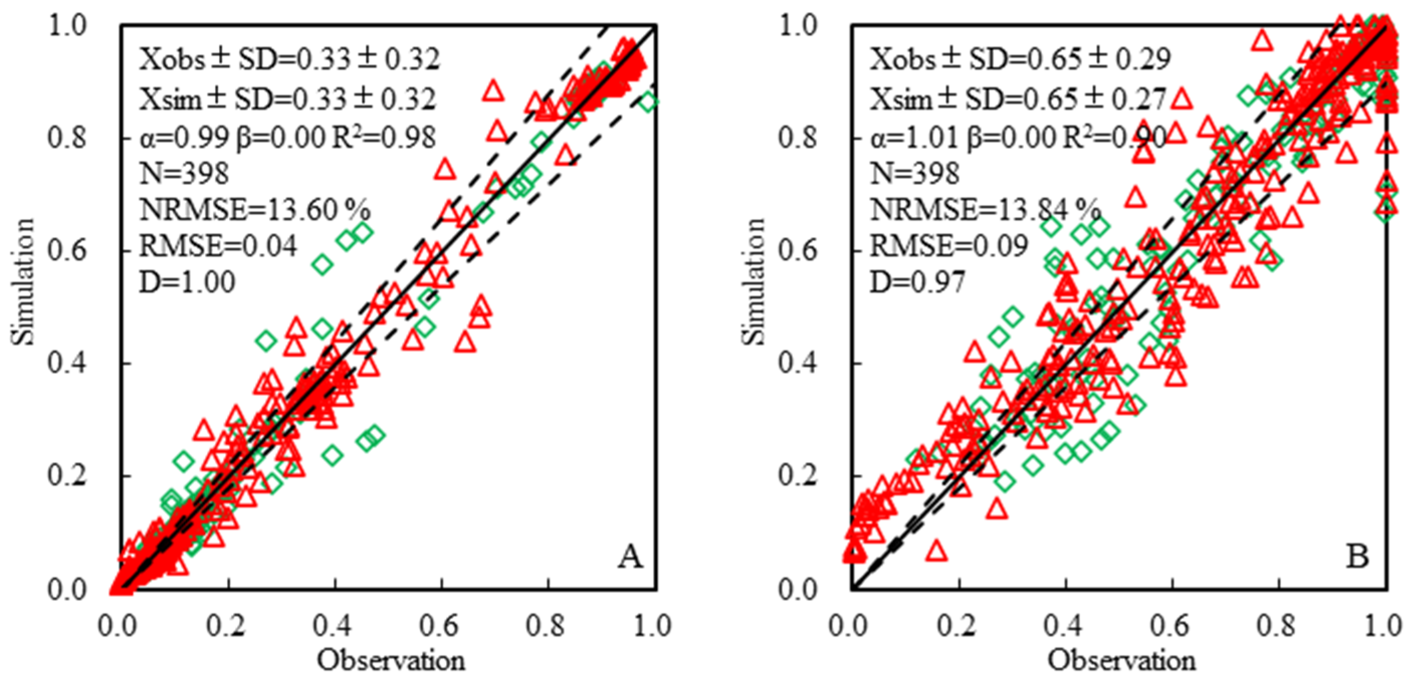
3.2. Model Validation

Based on the fitted equation parameters of cucumber fruit quality in Table 3, the cucumber fruit quality simulation model was validated using independent experimental data (

Table 4. Statistics of measured and simulated values of the VQSM model, where * indicates that the model exhibited an extremely high simulation effect, # indicates that the model showed a high simulation effect, $ indicates that the model exhibited a general simulation effect, and ! indicates that the model demonstrated a poor simulation effect.

Indicators			Unit	${\overline{\mathbf{X}}}_{\mathbf{o}\mathbf{b}\mathbf{s}}$ ± SD	${\overline{\mathbf{X}}}_{\mathbf{s}\mathbf{i}\mathbf{m}}$ ± SD	α	β	R2	RMSE	NRMSE (%)	D
Appearance	Cucumber	$F_{friut}$	N	15.05 ± 3.53	14.82 ± 2.99	1.12	−1.56	0.90	1.16	7.69 *	0.97
		$L_{friut}$	cm	13.20 ± 5.83	12.4 ± 4.68	1.00	0.76	0.65	3.46	26.23 $	0.88
		$D_{friut}$	cm	1.40 ± 0.51	1.33 ± 0.50	0.85	0.26	0.71	0.28	20.15 $	0.91
		${SI}_{friut}$	——	9.88 ± 0.76	9.86	——	——	——	0.74	7.47 *	——
		${CV}_{friut}$	——	11,828 ± 2685	12,035 ± 2101	1.13	−1799	0.78	1257	10.63 #	0.92
		${DV}_{friut}$	——	88.52 ± 1.93	88.81 ± 1.56	0.90	8.24	0.54	1.32	1.49 *	0.83
		$H_{friut}$	——	4.46 ± 2.13	4.51 ± 2.04	0.83	0.73	0.63	1.30	29.21 $	0.89
	Celery	$F_{stem}$	N	12.74 ± 0.77	12.97 ± 0.54	1.11	−1.63	0.60	0.50	3.96 *	0.82
		$N_{stem}$	——	8.8 ± 1.83	9.05 ± 1.93	0.86	0.98	0.83	0.79	9.00 *	0.95
		${CV}_{stem}$	——	35,609± 18,311	30,566 ± 12,290	1.29	−3971	0.76	10234	28.74 $	0.86
		${DV}_{stem}$	——	87.35 ± 4.76	84.99	——	——	——	4.94	5.66 *	——
		$H_{stem}$	——	2.19 ± 1.31	1.96 ± 1.12	1.11	0.01	0.90	0.46	21.04 $	0.96
		$H_{plant}$	cm	68.37 ± 25.09	64.61 ± 20.79	1.14	−5.16	0.89	9.43	13.79 #	0.96
		$N_{leaf}$	——	57.92 ± 21.45	59.28 ± 22.56	0.89	4.87	0.89	7.59	13.11 #	0.97
		$LA$	cm2	2317 ± 1355	2455 ± 1403	0.87	175	0.82	612	26.41 $	0.95
		${CV}_{leaf}$	——	18,968 ± 9831	18,489 ± 7785	1.25	−4073	0.97	2324	12.25 #	0.98
		${DV}_{leaf}$	——	85.14 ± 8.09	87.33	——	——	——	7.70	9.05 *	——
		$H_{leaf}$	——	3.36 ± 2.16	3.26 ± 1.75	1.05	−0.04	0.72	1.06	31.47 !	0.91
		$W_{stem}$	g	443.44 ± 353.06	479.70 ± 299.94	1.12	−92.50	0.90	119.76	27.01 $	0.96
		$W_{leaf}$	g	59.77 ± 35.47	61.05 ± 31.54	1.02	−2.51	0.82	14.68	24.57 $	0.95
		$W_{overground}$	g	503.22 ± 386.86	540.74 ± 331.48	1.11	−95.94	0.90	129.56	25.75 $	0.97
Physicochemical	Cucumber	${WC}_{fruit}$	%	95.31 ± 1.11	95.36	——	——	——	1.08	1.13 *	——
		${SSC}_{fruit}$	%	3.06 ± 0.29	3 ± 0.24	1.13	−0.34	0.86	0.12	3.93 *	0.94
		${SP}_{fruit}$	mg/g	1.28 ± 0.51	1.26 ± 0.4	1.17	−0.20	0.87	0.18	13.96 #	0.95
		${SS}_{fruit}$	mg/g	8.68 ± 5.11	7.97 ± 4.48	0.97	0.96	0.72	2.56	29.53 $	0.91
		${VC}_{fruit}$	mg/kg	77.4 ± 6.65	76.67 ± 7.98	0.81	15.25	0.95	2.09	2.70 *	0.98
	Celery	$CC$	SPAD	35.75 ± 2.79	35.1 ± 1.77	0.81	7.33	0.26	2.44	6.83 *	0.67
		${WC}_{leaf}$	%	94.23 ± 2.19	93.9 ± 1.6	0.98	2.54	0.51	1.54	1.63 *	0.81
		${WC}_{stem}$	%	81.81 ± 6.29	83.5	——	——	——	6.39	7.81 *	——
		${WC}_{overground}$	%	88.02 ± 3.88	88.71 ± 1.65	2.06	−94.78	0.77	2.60	2.96 *	0.77
		${SSC}_{leaf}$	%	2.28 ± 0.44	2.34 ± 0.41	1.03	−0.13	0.94	0.11	4.94 *	0.98
		${SSC}_{stem}$	%	4.43 ± 1.14	4.47 ± 1.13	0.96	0.15	0.89	0.36	8.04 *	0.97
		${SSC}_{overground}$	%	3.35 ± 0.69	3.4 ± 0.66	0.98	0.01	0.88	0.23	6.74 *	0.97

and Figure 1). From Table 4, it can be observed that the simulated values are close to the measured values and fall within the range of error, indicating a good agreement between the simulated and measured values. For the cucumber quality model, the root mean square error (RMSE) for the simulated models of $F_{friut}$, $L_{friut}$, $D_{friut}$, ${SI}_{friut}$, ${CV}_{friut}$, ${DV}_{friut}$, $H_{friut}$, ${WC}_{fruit}$, ${SSC}_{fruit}$, ${SP}_{fruit}$, ${SS}_{fruit}$, and ${VC}_{fruit}$ are 1.16 N, 3.46 cm, 2.81 mm, 0.74, 1257, 1.32, 1.30, 1.08%, 0.12%, 0.18 mg/g, 2.56 mg/g, and 2.09 mg/kg. The normalized root mean square error (NRMSE) ranges from 1.13% to 29.53% and the order of the simulation accuracy is ${WC}_{fruit}$, ${DV}_{friut}$, ${VC}_{fruit}$, ${SSC}_{fruit}$, ${SI}_{friut}$, $F_{friut}$, ${CV}_{friut}$, ${SP}_{fruit}$, $D_{friut}$, $L_{friut}$, $H_{friut}$, and ${SS}_{fruit}$. The D values range from 0.83 to 0.98. In conclusion, the simulation models for $F_{friut}$, ${SI}_{friut}$, ${DV}_{friut}$, ${WC}_{fruit}$, ${SSC}_{fruit}$, and ${VC}_{fruit}$ show excellent good simulation performance, and the simulation models for ${CV}_{friut}$ and ${SP}_{fruit}$ demonstrate good simulation performance. However, the simulation models for $L_{friut}$, $D_{friut}$, $H_{friut}$, and ${SS}_{fruit}$ exhibit moderate simulation performance. For the celery quality model, the root mean square error (RMSE) for the simulated models of $F_{stem}$, $N_{stem}$, ${CV}_{stem}$, ${DV}_{stem}$, $H_{stem}$, $H_{plant}$, $N_{leaf}$, $LA$, ${CV}_{leaf}$, ${DV}_{leaf}$, $H_{leaf}$, $W_{stem}$, $W_{leaf}$, $W_{overground}$, $CC$, ${WC}_{leaf}$, ${WC}_{stem}$, ${WC}_{overground}$, ${SSC}_{leaf}$, ${SSC}_{stem},$ and ${SSC}_{overground}$ are 0.50 N, 0.79, 10,234, 4.94, 0.46, 9.43 cm, 7.59, 612 cm², 2324, 7.70, 1.06, 119.76 g, 14.68 g, 129.56 g, 2.44 SPAD, 1.54%, 6.39%, 2.60%, 0.11%, 0.36%, and 0.23%, respectively. The NRMSE range from 1.63% to 31.47%, the order of the simulation accuracy is ${WC}_{leaf}$, ${WC}_{overground}$, $F_{stem}$, ${SSC}_{leaf}$, ${DV}_{stem}$, ${SSC}_{overground}$, $CC$, ${WC}_{stem}$, ${SSC}_{leaf}$, $N_{leaf}$, ${DV}_{leaf}$, ${CV}_{leaf}$, $N_{leaf}$, $H_{plant}$, $H_{stem}$, $W_{leaf}$, $W_{overground}$, $LA$, $W_{stem}$, ${CV}_{stem}$ and $H_{leaf}$. The D values range from 0.67 to 0.98. In conclusion, the simulated models for $F_{stem}$, $N_{stem}$, ${DV}_{stem}$, ${DV}_{leaf}$, $CC$, ${WC}_{leaf}$, ${WC}_{stem}$, ${WC}_{overground}$, ${SSC}_{leaf}$, ${SSC}_{stem}$, and ${SSC}_{overground}$ demonstrate excellent good simulation performance, the simulated models for $N_{leaf}$, $H_{plant},$ and ${CV}_{leaf}$ exhibit good simulation performance, the simulation performance for ${CV}_{stem}$, $H_{stem}$, $LA$, $W_{stem}$, $W_{leaf}$ and $W_{overground}$ is moderate, and $H_{leaf}$ exhibits poor simulation performance.

This study classified the indicators based on the results in Figure 1. The obtained root mean square errors (RMSE) for the models of firmness, length, diameter, shape index, color value, darker value, hue, number, leaf area, water content, soluble solid content, soluble protein content, soluble sugar content, vitamin C, and chlorophyll content are 1.02 N, 7.48 cm, 2.81 mm, 0.74, 4793, 4.22, 1.13, 6.49, 612 cm², 102.22 g, 3.68%, 0.23%, 0.18 mg/g, 2.56 mg/g, 2.09 mg/kg, and 2.44 SPAD, respectively. The NRMSE ranges from 2.70% to 30.47%. Among the models, those for firmness, shape index, darkness value, water content, soluble sugar content, vitamin C, and chlorophyll content demonstrate extremely high accuracy in the simulation, while the models for length, number, and soluble solid content exhibit excellent accuracy. The simulation accuracy for the models of diameter, color value, hue, leaf area, and soluble protein content is considered average.

To better demonstrate the overall simulation effect of the VQSM model, this study normalized all quality index data. Due to some indices (including water content, darkness value, and fruit shape index) being insensitive to the comprehensive environmental factors, they are not considered as target indices for evaluating the overall performance of the model. Based on data characteristics, this study filtered two types of normalization methods (Equations (29) and (30)).

$$Y_{i\_1}=X_i/{10}^k$$

(29)

$$Y_{i\_2}=X_i/\max \left(X_i\right)$$

(30)

where i = 1, 2, …, N, and N is the number of indicator samples. $\max \left(X_i\right)$ represents the maximum value of the indicator, $\min \left(X_i\right)$ represents the minimum value of the indicator, $X_i$ represents the indicator value, and $Y_i$ represents the normalized value of the indicator, [0, 1], where the decimal proportions normalization is denoted as $Y_{i\_1}$, whereas the maximum normalization is denoted as $Y_{i\_2}$.

Based on the results shown in Figure 2, both normalization methods exhibit an average RMSE of 0.07, an average NRMSE of 13.72%, and an average D of 0.99. These values indicate that the VQSM model possesses a high degree of simulation accuracy, making it suitable for widespread application in production. Specifically, for simulating cucumber quality, the RMSE is 0.08, while the NRMSE is 15.64%, while for simulating celery quality, the RMSE is 0.07, while the NRMSE is 13.93%. These results indicate that the model effectively captures the quality of leafy vegetables.

4. Discussion

This study constructed a dynamic simulation model for the formation of vegetable organ quality in solar greenhouses (VQSM). According to the research, the temperature and the radiation are key environmental factors that affect crop growth, development, and yield quality [13,14]. Therefore, this study introduces the accumulate temperature difference method (ATD) [29], which only considers the temperature, and the accumulated product of thermal effectiveness and the photosynthetically active radiation method (TEP), which considers both temperature and radiation, to quantify the process of crop quality formation. Previous studies have used the radiation heat accumulation method to construct crop growth and development models, which have shown good simulation results [26,27,28]. However, these models consider the daily average temperature without considering the consistency between radiation and temperature. Therefore, this study replaces the daily average temperature with daytime temperature based on the variation law of radiation throughout the day. In addition, this study further compares and selects the optimal simulation methods to comprehensively consider the photothermal sensitivity of crop organ development, aiming to improve the accuracy of the model simulation. However, further research is needed to explore the influence of different temperature types (leaf temperature [29], soil temperature [39], extreme temperature [40], etc.) and different light conditions (spectrum, intensity, and duration [41,42]) on crop quality formation.

Currently, research has developed systematic semi-mechanistic crop models based on physiological and ecological processes [17,18]. These models have complex and diverse parameter types, which are not easily obtained and involve a large amount of experimental data for parameter localization. In terms of input data for modeling, in addition to conventional temperature radiation data, additional inputs include CO₂ concentration and air humidity. Regarding model parameters, it is necessary to determine difficult-to-obtain parameters such as the coefficient in the expolinear equation, the light transmission coefficient, the maintenance respiration coefficient, the parameter involved in the photosynthesis reduction factor, etc. [17]. In order to improve the applicability of the models, this study uses the principle of least squares to determine the quantitative relationship between developmental process indicators and quality formation indicators, greatly reducing the types of crop parameters. Accurate quality indicators can be fitted by inputting easily obtainable temperature and radiation data. The NRMSE of the cucumber quality model ranges from 1.13% to 29.53%, and the NRMSE of the celery quality model ranges from 1.63% to 31.47%. The accuracy levels of the model simulation indicators are divided, with 17 indicators showing exceedingly good simulation effects (accounting for 51.52% of the total indicators), 5 indicators showing good simulation effects, 10 indicators showing moderate simulation effects, and 1 indicator showing poor simulation effects.

Data normalization transforms data into a specific range or distribution for subsequent data analysis and model training. Data normalization can eliminate the influence of dimensions, enabling the fair comparison of indicators with different dimensions. It ensures that all features have equal importance during the model training process, avoiding the dominance of certain features due to large numerical ranges, thereby improving model performance, stability, and training efficiency. It also helps map data from different scales to the same scale, making data distribution more intuitive, facilitating observation and analysis [26,30,31]. Currently, there is less emphasis on evaluating the overall system accuracy of a model in terms of a specific indicator, with most studies focusing on individual indicators [26,27,28,29,30,31]. Therefore, based on the data distribution characteristics, this study selects two kinds of normalization methods to comprehensively evaluate the accuracy of the system VQSM model, and the model has an NRMSE of 12.22% (indicating high accuracy).

Regarding future research and the application directions of the VQSM model, efforts should be focused on further exploring the coupling mechanisms and methods with “3S” technologies [43]. This should involve considering factors such as water and fertilizer management conditions and the genetic characteristics of the cultivars [44]. Additionally, it is recommended to incorporate productivity models, such as CPSM [32], to construct an economic benefit simulation model [45].

5. Conclusions

(1)

There exist quantifiable relationships between different quality indicators and ATD or TEP. These relationships are mainly presented through linear functions ($F_{friut}$, ${CV}_{friut}$, $H_{friut}$, $F_{stem}$, $W_{stem}$, $W_{leaf}$, $W_{overground}$, $H_{stem}$ and $H_{leaf}$), exponential functions ($L_{friut}$ and $D_{friut}$), the logarithmic function (${DV}_{friut}$), and logical functions ($N_{stem}$, $N_{leaf}$, $H_{plant}$, $LA$, ${CV}_{stem}$, and ${CV}_{leaf}$).

(2)

The normalized root mean square error (NRMSE) of the quality model for cucumber ranges from 1.13% to 29.53%, and the simulation models for $F_{friut}$, ${SI}_{friut}$, ${DV}_{friut}$, ${WC}_{fruit}$, ${SSC}_{fruit}$, and ${VC}_{fruit}$ show excellent good simulation performance. The NRMSE of the quality model for celery ranges from 1.63% to 31.47%, and the simulated models for $F_{stem}$, $N_{stem}$, ${DV}_{stem}$, ${DV}_{leaf}$, $CC$, ${OW}_{leaf}$, ${OW}_{stem}$, ${OW}_{overground}$, ${SSC}_{leaf}$, ${SSC}_{stem},$ and ${SSC}_{overground}$ show excellent simulation performance.

(3)

Based on the normalization methods, the average NRMSE of the VQSM model is 13.72%, demonstrating a relatively high level of accuracy in the simulation, making it suitable for practical applications.

References

1. Li, Z.F.; Liu, T.; Dong, C.Y.; Xue, Q.Y.; Liu, S.M. Climate classification of solar greenhouse based on the calculation method for indoor and outdoor temperature difference at night. Trans. Chin. Soc. Agric. Eng. 2021, 37, 194–201. [Google Scholar]
2. Zhu, Z.P.; Yu, J.X.; Qiao, X.H.; Yu, Z.F.; Xiong, A.S.; Sun, M. Hydrogen sulfide delays yellowing and softening, inhibits nutrient loss in postharvest celery. Sci. Hortic. 2023, 315, 111991. [Google Scholar] [CrossRef]
3. Gnayem, N.; Magadley, E.; Haj-Yahya, A.; Masalha, S.; Kabha, R.; Abasi, A.; Barhom, H.; Matar, M.; Attrash, M.; Yehia, I. Examining the effect of different photovoltaic modules on cucumber crops in a greenhouse agrivoltaic system: A case study. Biosyst. Eng. 2024, 241, 83–94. [Google Scholar] [CrossRef]
4. Saadi, S.; Pattey, E.; Jego, G.; Champagne, C. Prediction of rainfed corn evapotranspiration and soil moisture using the STICS crop model in eastern Canada. Field Crops Res. 2022, 287, 108664. [Google Scholar] [CrossRef]
5. Dhakar, R.; Sehgal, V.K.; Chakraborty, D.; Sahoo, R.N.; Mukherjee, J.; Ines, A.V.M.; Kumar, S.N.; Shirsath, P.B.; Roy, S.B. Field scale spatial wheat yield forecasting system under limited field data availability by integrating crop simulation model with weather forecast and satellite remote sensing. Agric. Syst. 2022, 195, 103299. [Google Scholar] [CrossRef]
6. Pohankova, E.; Hlavinka, P.; Kersebaum, K.C.; Rodriguez, A.; Jan, B.; Bednarik, M.; Dubrovsky, M.; Gobin, A.; Hoogenboom, G.; Moriondo, M.; et al. Expected effects of climate change on the production and water use of crop rotation management reproduced by crop model ensemble for Czech Republic sites. Eur. J. Agron. 2022, 134, 126446. [Google Scholar] [CrossRef]
7. Onyekwelu, I.; Sharda, V. Root proliferation adaptation strategy improved maize productivity in the US Great Plains: Insights from crop simulation model under future climate change. Sci. Total Environ. 2024, 927, 172205. [Google Scholar] [CrossRef]
8. Shen, H.; Wang, Y.; Jiang, K.; Huang, D.; Wu, J.; Wang, Y.; Ma, X. Simulation modeling for effective management of irrigation water for winter wheat. Agric. Water Manag. 2022, 269, 107720. [Google Scholar] [CrossRef]
9. Wan, Y.; Zhou, M.; Le, L.; Gong, X.; Jiang, L.; Huang, J.; Cao, X.; Shi, Z.; Tan, M.; Cao, Y.; et al. Evaluation of morphology, nutrients, phytochemistry and pigments suggests the optimum harvest date for high-quality quinoa leafy vegetable. Sci. Hortic. 2022, 304, 111240. [Google Scholar] [CrossRef]
10. Vanmarcke, H.; Tuytschaever, T.; Everaert, B.; Cuypere, T.D.; Sampers, I. Impact of using stored treated municipal wastewater for irrigation on the microbial quality and safety of vegetable crops. Agric. Water Manag. 2024, 297, 108842. [Google Scholar] [CrossRef]
11. Wang, Q.; Chen, J.Y.; Xu, M.S.; Shen, Y.G.; Zhou, M.; Zhu, F.N.; Luo, J.Q.; Chen, H.Z. Effect of huanglongbing on the quality of Newhall Navel Orange. Food Sci. 2019, 40, 48–53. [Google Scholar]
12. Juventia, S.D.; Rossing, W.A.H.; Ditzler, L.; van Apeldoorn, D.F. Spatial and genetic crop diversity support ecosystem service delivery: A case of yield and biocontrol in Dutch organic cabbage production. Field Crops Res. 2021, 261, 108015. [Google Scholar] [CrossRef]
13. Kawasaki, Y.; Yoneda, Y. Local temperature control in greenhouse vegetable production. Hortic. J. 2019, 88, 305–314. [Google Scholar] [CrossRef]
14. Chen, Z.; Jahan, M.S.; Mao, P.P.; Wang, M.M.; Liu, X.Y.; Guo, S.R. Functional growth, photosynthesis and nutritional property analyses of lettuce grown under different temperature and light intensity. J. Hortic. Sci. Biotechnol. 2021, 96, 53–61. [Google Scholar] [CrossRef]
15. Qu, Z.; Chen, Q.; Feng, H.; Hao, M.; Niu, G.L.; Liu, Y.L.; Li, C.L. Interactive effect of irrigation and blend ratio of controlled release potassium chloride and potassium chloride on greenhouse tomato production in the Yellow River Basin of China. Agric. Water Manag. 2022, 261, 107346. [Google Scholar] [CrossRef]
16. Wang, R.; Shi, W.; Kronzucker, H.J.; Li, Y. Oxygenation promotes vegetable growth by enhancing P nutrient availability and facilitating a stable soil bacterial community in compacted soil. Soil Tillage Res. 2023, 230, 105686. [Google Scholar] [CrossRef]
17. Vazquez-Cruz, M.A.; Guzman-Cruz, R.; Lopez-Cruz, I.L.; Cornejo-Perez, O.; Torres-Pacheco, I.; Guevara-Gonzalez, R.G. Global sensitivity analysis by means of EFAST and Sobol’ methods and calibration of reduced state-variable TOMGRO model using genetic algorithms. Comput. Electron. Agric. 2014, 100, 1–12. [Google Scholar] [CrossRef]
18. Berrueta, C.; Heuvelink, E.; Giménez, G.; Dogliotti, S. Estimation of tomato yield gaps for greenhouse in Uruguay. Sci. Hortic. 2020, 265, 109250. [Google Scholar] [CrossRef]
19. Cooman, A.; Schrevens, E. A monte Carlo approach for estimating the uncertainty of predictions with the tomato plant growth model, TOMGRO. Biosyst. Eng. 2006, 94, 517–524. [Google Scholar] [CrossRef]
20. Ioslovich, I.; Gutman, P.O. Fitting the MBM-a model of plant growth to the data of TOMGRO: Implication for greenhouse optimal control. Acta Hortic. 2008, 801, 515–521. [Google Scholar] [CrossRef]
21. Chapagain, R.; Remenyi, T.A.; Harris, R.M.B.; Mohammed, C.L.; Huth, N.; Wallach, D.; Rezaei, E.E.; Ojeda, J.J. Decomposing crop model uncertainty: A systematic review. Field Crops Res. 2022, 279, 108448. [Google Scholar] [CrossRef]
22. Miao, M.; Zhang, Z.; Xu, X.; Wang, K.; Cheng, H.; Cao, B. Different mechanisms to obtain higher fruit growth rate in two cold-tolerant cucumber (Cucumis sativus L.) lines under low night temperature. Sci. Hortic. 2009, 119, 357–361. [Google Scholar] [CrossRef]
23. Aparna, G.; Matthew, D.K.; Joseph, S.; Ling, P.P.; Streeter, J.G. Temperature and genotype affect anthocyanin concentrations in lettuce (Lactuca sativa). HortScience 2004, 39, 864A. [Google Scholar]
24. Arya, S.S.; Parihar, D.B. Effect of moisture and temperature on storage changes in lipids and carotenoids of atta (wheat flour). Mol. Nutr. Food Res. 2010, 25, 121–126. [Google Scholar] [CrossRef]
25. Piva, A.; Bertrand, A.; Gilles, B.; Yves, C.; Philippe, S. Growth and physiological response of timothy to elevated carbon dioxide and temperature under contrasted nitrogen fertilization. Crop Sci. 2013, 53, 704–715. [Google Scholar] [CrossRef]
26. Cheng, C.; Dong, C.Y.; Li, Z.F.; Gong, Z.H.; Feng, L.P. Simulation model of external morphology and dry matter accumulation and distribution of celery in solar greenhouse. Trans. Chin. Soc. Agric. Eng. 2021, 37, 142–151. [Google Scholar]
27. Shi, X.H.; Cai, H.J.; Zhao, L.L.; Yang, P.; Wang, Z.S. Greenhouse tomato dry matter production and distribution model under condition of irrigation based on product of thermal effectiveness and photosynthesis active radiation. Trans. Chin. Soc. Agric. Eng. 2016, 32, 69–77. [Google Scholar]
28. Liu, F.H.; Guo, S.B.; Wang, D.; Huang, B.; Cao, Y.F. Construction and verification of an external morphology, substance accumulation, and distribution model of tomatoes in greenhouses. Trans. Chin. Soc. Agric. Eng. 2022, 38, 188–196. [Google Scholar]
29. Cheng, C.; Li, C.; Li, W.M.; Ye, C.Y.; Wang, Y.S.; Zhao, C.S.; Ding, F.H.; Jin, Z.F.; Feng, L.P.; Li, Z.F. Optimal path of the simulation model in horticultural crop development and harvest period. Trans. Chin. Soc. Agric. Eng. 2023, 39, 158–167. [Google Scholar]
30. Jia, K.; Lin, J.; Tan, M.; Tao, D.C. Deep multi-view learning using Neuron-Wise Correlation-Maximizing Regularizers. IEEE Trans. Image Process. 2019, 28, 5121–5134. [Google Scholar] [CrossRef]
31. Kaur, R.; Chen, Z.; Motl, R.; Hernandez, M.E.; Sowers, R. Predicting multiple sclerosis from gait dynamics using an instrumented treadmill—A machine learning approach. IEEE Trans. Biomed. Eng. 2020, 68, 2666–2667. [Google Scholar] [CrossRef]
32. Cheng, C.; Dong, C.Y.; Guan, X.L.; Chen, X.G.; Wu, L.; Zhu, Y.C.; Zhang, L.; Ding, F.H.; Feng, L.P.; Li, Z.F. CPSM: A dynamic simulation model for cucumber productivity in solar greenhouse based on the principle of effective accumulated temperature. Agronomy 2024, 14, 1242. [Google Scholar] [CrossRef]
33. Duarte, G.N.; Maluf, W.R.; Duarte, G.R.B.; de Oliveira, A.S.; Licursi, V. Fruit color and firmness in tomato hybrids as a function of the alleles rin, nor, norA, ogc and hp. Sci. Hortic. 2023, 319, 112159. [Google Scholar] [CrossRef]
34. Wu, L.; Liu, J.Y.; Liang, Y. Inheritance on fruit color character between green and red of tomato. Acta Hortic. Sin. 2016, 43, 674–682. [Google Scholar]
35. Hasan, S.M.K.; Manzocco, L.; Morozova, K.; Nicoli, M.C.; Scampicchio, M. Effects of ascorbic acid and light on reactions in fresh-cut apples by microcalorimetry. Thermochim. Acta 2017, 649, 63–68. [Google Scholar] [CrossRef]
36. Ezzat, A.O.; Tawfeek, A.; Mohammad, F.; Al-Lohedan, H.A. Modification of magnetite nanoparticles surface with multifunctional ionic liquids for coomassie brilliant blue R-250 dye removal from aqueous solutions. J. Mol. Liq. 2022, 358, 119195. [Google Scholar] [CrossRef]
37. Li, H.S. Principles and Techniques of Plant Physiological Biochemical Experiment; Higher Education Press: Beijing, China, 2000. [Google Scholar]
38. Li, X.Y.; Meng, L.; Shen, L.; Ji, H.F. Regulation of gut microbiota by vitamin C, vitamin E and β-carotene. Food Res. Int. 2023, 169, 112749. [Google Scholar] [CrossRef] [PubMed]
39. Ai, P.; Ma, Y.; Hai, Y. Influence of jujube/cotton intercropping on soil temperature and crop evapotranspiration in an arid area. Agric. Water Manag. 2021, 256, 107118. [Google Scholar] [CrossRef]
40. Pan, T.; Chen, Q.; Chen, J.; Pan, T.; Ge, Q.S. Plausible changes in wheat-growing periods and grain yield in China triggered by future climate change under multiple scenarios and periods. Q. J. R. Meteorol. Soc. 2021, 147, 4371–4387. [Google Scholar]
41. Kishore, K.; Rupa, T.R.; Samant, D. Influence of shade intensity on growth, biomass allocation, yield and quality of pineapple in mango-based intercropping system. Sci. Hortic. 2021, 278, 109868. [Google Scholar] [CrossRef]
42. Boros, I.F.; Szekely, G.; Balazs, L.; Csambalik, L.; Sipos, L. Effects of LED lighting environments on lettuce (Lactuca sativa L.) in PFAL systems-A review. Sci. Hortic. 2023, 321, 112351. [Google Scholar] [CrossRef]
43. Lv, Z.; Liu, X.; Cao, W.; Zhu, Y. A model-based estimate of regional wheat yield gaps and water use efficiency in main winter wheat production regions of China. Sci. Rep. 2017, 7, 6081. [Google Scholar] [CrossRef] [PubMed]
44. Ghasemi-Saadatabadi, F.; Zand-Parsa, S.; Gheysari, M.; Sepaskhah, A.R.; Mahbod, M.; Hoogenboom, G. Improving prediction accuracy of CSM-CERES-Wheat model for water and nitrogen response using a modified Penman-Monteith equation in a semi-arid region. Field Crops Res. 2024, 312, 109381. [Google Scholar] [CrossRef]
45. Tang, S.; Zheng, N.; Ma, Q.; Zhou, J.J.; Sun, T.; Zhang, X.; Wu, L.H. Applying Nutrient Expert system for rational fertilisation to tea (Camellia sinensis) reduces environmental risks and increases economic benefits. J. Clean. Prod. 2021, 305, 127197. [Google Scholar] [CrossRef]
Figure 1. The response of the VQSM model accuracy by NRMSE to commodity organ quality formation indicators, where the smaller the proportion in the graph, the higher the simulation effect becomes.
Agriculture 14 01531 g001
Figure 2. Comparison between measured and simulated normalization values of VQSM model, including decimal proportions normalization (A) and max normalization (B). The green mark represents the cucumber quality index data, and the red mark represents the celery quality index data.
Agriculture 14 01531 g002