A High-Precision, Ultra-Short Baseline Positioning Method for Full Sea Depth

Abstract

To fulfill the demand for high-precision underwater acoustic positioning at full sea depth, an ultra-short baseline (USBL) positioning method with the square array based on the least squares estimating signal parameters via rotational invariance techniques (LS-ESPRIT) algorithm is presented in this paper. A combination of beam tracking and beamforming is employed to improve the accuracy of direction-of-arrival (DOA) estimation and, consequently, enhance overall positioning accuracy. In order to mitigate the issue of position jumping resulting from phase ambiguity in traditional four-element cross arrays, we have improved the stability of the positioning algorithm by utilizing a multi-element square array and employing the LS-ESPRIT algorithm for DOA estimation. Furthermore, the signal detection method integrating the correlation coefficient and ascending/descending chirp signals is employed to enhance the reliability of the location algorithm. Simulation analysis and experimental results demonstrate that the proposed algorithm effectively enhances positioning accuracy and improves the problem of jumping in positioning results.

1. Introduction

Manned submersibles are essential equipment for conducting deep-sea scientific research and investigation and are an important tool for deep-sea exploration and exploitation. Various submersibles operating in the deep sea require real-time positioning, and the marine environmental characteristics require that the positioning of deep-sea manned submersibles rely on sound waves [1,2,3,4]. Underwater acoustic positioning offers indispensable technical support for precise operations such as the underwater detection and navigation control of submarines.

Underwater acoustic positioning technology can be classified into three types based on the length of the receiving array baseline: the long baseline positioning system, the short baseline positioning system, and the ultra-short baseline positioning system. The ultra-short baseline positioning system possesses the advantages of simple composition, convenient installation, effortless operation, and maneuverability. It is in line with the operation characteristics of large-depth submersibles with large operation ranges [5,6,7]. The ultra-short baseline positioning system typically demands more than three receiving transducers to form a receiving transducer array and is fixed at the bottom of the surface ship. The acoustic beacon installed on the submersible transmits an acoustic signal, and each transducer in the ultra-short baseline positioning array receives the acoustic beacon signal. Distance and orientation are established by calculating the time difference and phase difference between the signal transmitted and the signal received by different transducers, and, subsequently, the absolute position of the acoustic beacon is obtained by sound velocity correction and coordinate transformation [8,9,10].

The conventional ultra-short baseline positioning approach employs four primitive planar arrays. In order to solve the phase ambiguity problem caused by the array spacing exceeding half wavelength, a series of algorithms are designed and improved. Yu Min et al. [11] proposed an eight-element, high-precision, ultra-short baseline positioning system based on the narrowband signal phase difference. A pair of arrays with an aperture of less than half a wavelength was employed to solve the ambiguity, and a pair of arrays with a large aperture was utilized to improve the positioning accuracy. This method greatly increases the number of array elements, increases the complexity of producing the transducer, and decreases its reliability. Zheng Cuie et al. [12] proposed the utilization of phase anti-ambiguity from double pulse signals to improve the positioning accuracy, reduce the number of array elements, and yet increase the complexity of the transmitter. Zheng Enming et al. [13] also employed small-space array elements to solve ambiguity and large-space array elements to improve positioning accuracy when optimizing traditional array elements. Luo Qinghua [14] introduced the Kalman filter into the ultra-short baseline positioning technology to improve positioning accuracy. Zhu Yu et al. [15] put forward a cross-spectrum, direction-finding approach based on phase splicing. This algorithm requires a high signal-to-noise ratio, and its performance deteriorates significantly when the signal-to-noise ratio is low. The azimuth estimation algorithms for array signals include multiple signal classification algorithms [16], subspace fitting algorithms [17,18], rotation invariant subspace algorithms [19,20], etc. The multiple signal classification algorithm and subspace fitting algorithm are optimization search problems, and the accuracy of azimuth estimation is related to the search step. The rotation invariant subspace algorithm does not require searching and has analytical solutions. In this paper, the 6*6 element square array is adopted, and beam tracking and beamforming are utilized to improve the processing gain. The reliability of the location algorithm is improved through applying a signal detection method using a correlation coefficient and ascending/descending chirp detection. The LS-ESPRIT (least squares and rotation-invariant subspace) algorithm is employed to estimate the spectrum and obtain the wave azimuth estimation results. This method makes the ultra-short baseline positioning system have a long operating distance, have a high positioning accuracy, and have a stable performance when some elements fail while avoiding phase ambiguity. The specific contributions of this paper are as follows:

(1)

The initial orientation of the current incoming wave is estimated by exploiting the positioning results of the previous 1 ping and the current attitude of the array. Then the phase shift beamforming is carried out to improve the signal processing gain.

(2)

According to the pulse compression results, the correlation coefficient is calculated to detect the arrival time of the signal. The non-system signal is eliminated according to the chirp gap to improve the reliability of the algorithm.

(3)

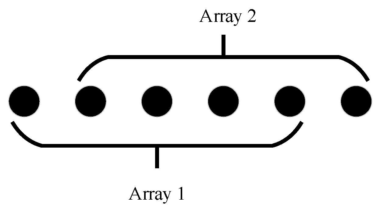
The multi-primitive square array is adopted, and the LS-ESPRIT algorithm is utilized to estimate the wave square position to improve the positioning accuracy and to improve the positioning result hopping problem.

2. Theoretical Analysis

The ultra-short baseline positioning system calculates the position of the sound source by measuring the time delay and phase difference of the sound wave generated by the sound source reaching the receiving array. This system is composed of two components: an underwater sound beacon and a surface signal receiving and processing unit, as shown in Figure 1. The underwater acoustic beacon emits sound signals controlled by high-precision, synchronized, clock-triggering signals. The propagation time delay is calculated by calculating the time difference between the signal received by the transducer array and the synchronization pulse. The overall azimuth estimation is achieved by estimating the direction of arrival of two perpendicular linear arrays. This section elaborates on the method in terms of sound signal generation and reception and signal processing.

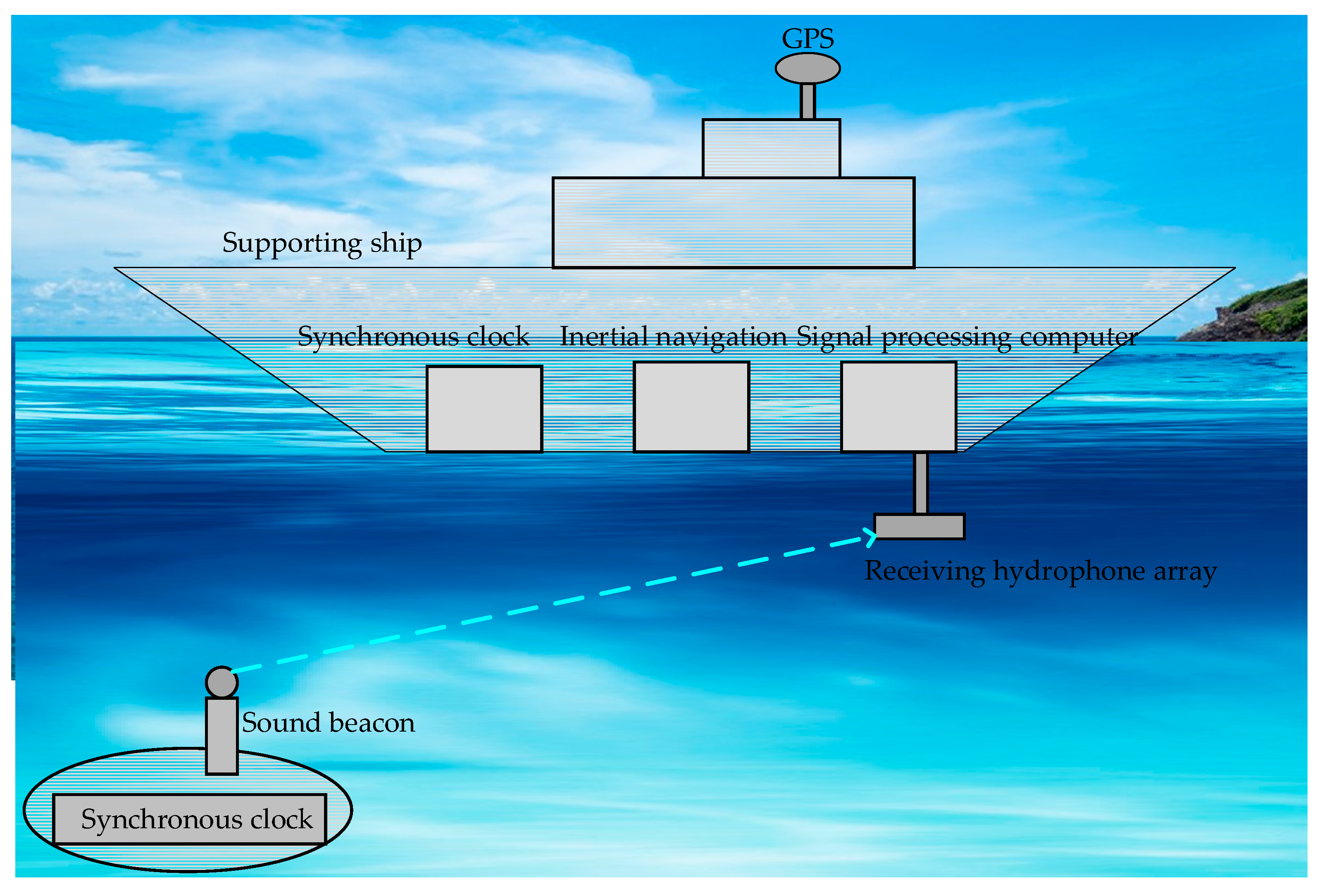
2.1. Generation and Reception of Acoustic Signals

The generation equation of linear frequency modulation signal (LFM) emitted by a sound beacon is shown in Equation (1).

$$s(t)=\cos (2\pi (at+b)t+\mathrm{\phi })$$

(1)

Here, coefficients a and b are the parameters that control frequency modulation and $\phi$ is the initial phase of the signal.

According to the definition of the LFM signal and frequency change mode, the LFM signal can be classified into the up-frequency-modulation signal and the down-frequency-modulation signal. The up-frequency-modulation signal is shown in Equation (2), and the down-frequency-modulation signal is shown in Equation (3).

$$s(t)=\cos \left(2\pi \left({\displaystyle \frac{F_{\max }-F_{\min }}{2T}}t+F_{\min }\right)t+\mathrm{\phi }\right)$$

(2)

$$s(t)=\cos \left(2\pi \left({\displaystyle \frac{F_{\min }-F_{\max }}{2T}}t+F_{\max }\right)t+\mathrm{\phi }\right)$$

(3)

Here, coefficient F_max is the highest frequency of the LFM signal, F_min is the lowest frequency of the LFM signal, T is the frequency modulation period, and $\phi$ is the initial phase of the signal.

The distribution of the receiving transducer array elements used in this paper is shown in Figure 2. There are 6 elements in each row and column, totaling 36 elements. The spacing between elements is 0.45$\lambda$, and the black element located in the bottom right corner serves as the reference element.

There exist three coordinate systems: the carrier coordinate system, the local coordinate system, and the World Geodetic System (WGS-84) coordinate system. The origin of the carrier coordinate system is USBL, with the positive x-axis oriented towards the starboard, the positive y-axis oriented towards the bow, and the positive z-axis perpendicularly upward to the vessel. The origin of the local coordinate system is located at the center of the vessel’s GPS, with the positive x-axis directed eastward, the positive y-axis directed northward, and the positive z-axis directed upward towards the sky. The WGS-84 coordinate system represents latitudes and longitudes on a global scale.

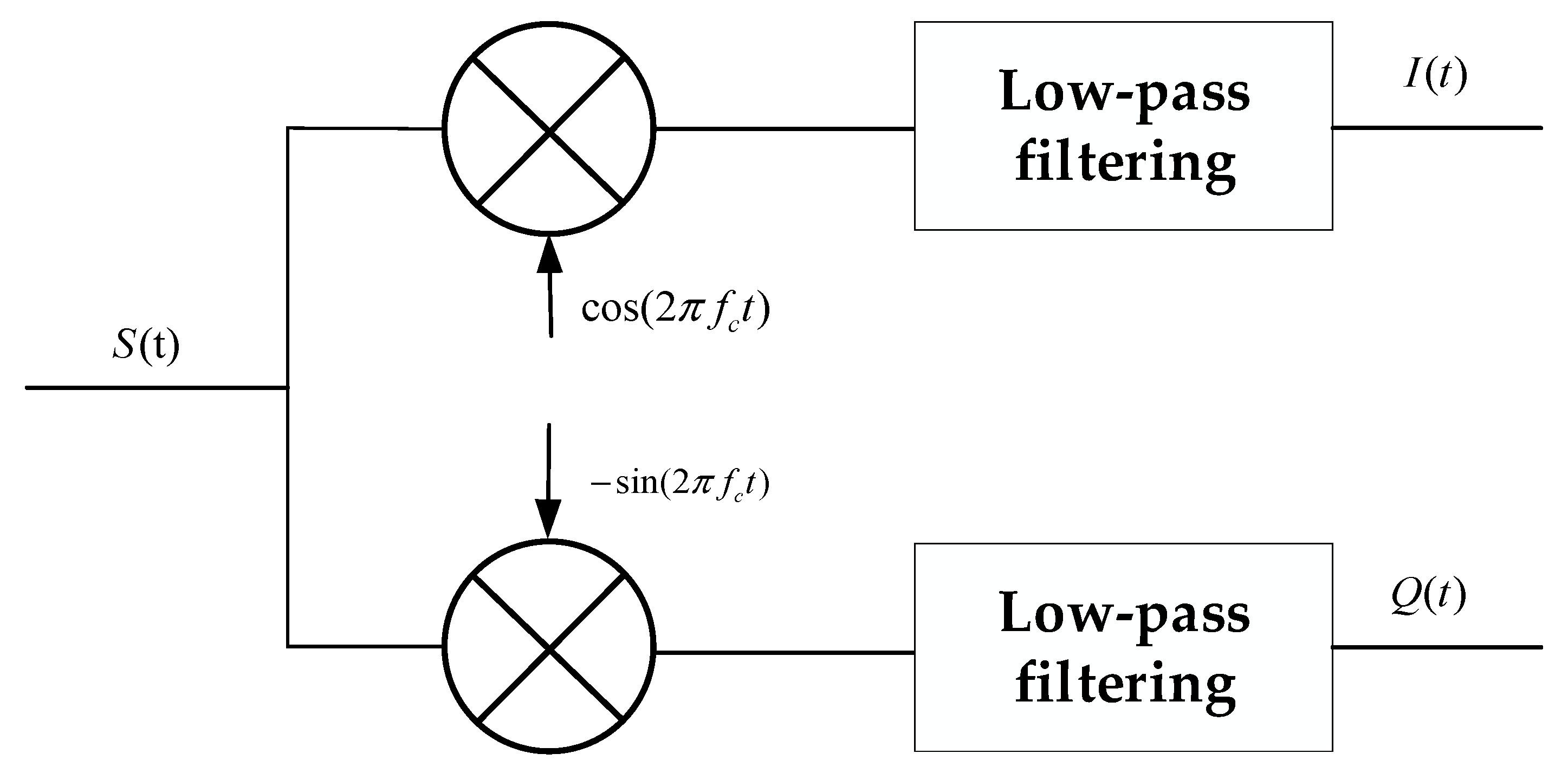
2.2. Signal Processing

The principle of orthogonal demodulation is shown in Figure 3.

Here, f_c is the central frequency of the LFM signal, I(t) is the in-phase channel, and Q(t) is the quadrature channel.

When the signal direction cannot be determined initially, the ultra-short baseline positioning system employs Discrete Fourier Transform (DFT) beamforming [21] to search the direction and then switches to the tracking state. In the tracking state, the processing gain is improved by phase-shift beamforming on each row and column of data. Owing to the application of broadband signals in the system, there may be certain loss in the effectiveness of processing gain. Afterwards, the pulse compression will be applied to the received signal. To facilitate comprehension, the formula has been simplified here and the results of pulse compression are directly represented using data without beamforming. The pulse compression results of a single channel are as follows:

$$u_o(t)=a\sqrt{B\tau }{\displaystyle \frac{\sin [\pi B(t-t_d)]}{\pi B(t-t_d)}}{e}^{-j2\pi f_c{t}_d}+n(t)$$

(4)

Here, $a$ represents the signal amplitude, $B$ represents the signal bandwidth, $\tau$ represents the signal pulse width, $t_d$ represents the signal transmission delay, and $n(t)$ represents the noise after pulse compression. Generally, the position of the signal is determined based on the ratio of the compressed pulse result to the noise. When the interference signal is stronger than the system signal, it may occur that the pulse compression result of the interference signal is stronger than that of the system signal. This will result in an incorrect position estimation of the signal. Therefore, the signal detection in this article employs the correlation coefficient [22] method:

$${\displaystyle \frac{\left|u_o(p)\right|}{\sqrt{\frac{1}{\tau }{\displaystyle \underset{p}{\overset{\tau +p}{\int }}{\left|s(t)\right|}^{2}dt}}}}>T_p$$

(5)

Here, $s(t)$ represents the signal after beamforming, $p$ represents the detection position, and $T_p$ represents the detection threshold. By dividing by the effective amplitude of the signal, the detection threshold of the correlation coefficient can effectively mitigate the influence of interference signals. The position of the maximum value within time $\tau$ after detecting the threshold point position represents the signal position. Taking the data within the main peak of the pulse compression results as the input signal for the LS-ESPRIT algorithm, the autocorrelation results are as follows:

$$R=E\left[X{X}^H\right]$$

(6)

Here, $X$ is the data within the main peak of the pulse compression result and ${\left[•\right]}^H$ represents the conjugate transpose operation of a matrix. The power method [23] is employed to decompose the autocorrelation results, thereby obtaining the signal subspace $U_s$. Decomposing each linear array into two sub-arrays allows us to obtain the signal subspace $U_{s1}$ and $U_{s2}$, as shown in Figure 4.

According to the least squares algorithm, the basic principle of LS-ESPRIT is as follows:

$$U_{s2}=U_{s1}\mathrm{\Psi }$$

(7)

From the mathematical knowledge of least squares (LS), we can see that the method of least squares solution of the above equation is equivalent to Equation (8).

$$\min {‖\Delta {\mathrm{U}}_{s2}‖}^2 s.t. U_{s1}\mathrm{\Psi }=U_{s2}+\Delta U_{s2}$$

(8)

Expanding upon Equation (8), the following equation can be obtained:

$$f(\mathrm{\Psi })={‖U_{s1}\mathrm{\Psi }-U_{s2}‖}^2=U_{s2}^H{U}_{s2}-U_{s2}^H{U}_{s1}\mathrm{\Psi }-{\mathrm{\Psi }}^H{U}_{s1}^H{U}_{s2}+{\mathrm{\Psi }}^H{U}_{s1}^H{U}_{s1}\mathrm{\Psi }$$

(9)

Taking the derivative of the above equation $\mathrm{\Psi }$ and making it equal to zero, we obtain the equation as follows:

$${\displaystyle \frac{df(\mathrm{\Psi })}{d\mathrm{\Psi }}}=-2U_{s1}^H{U}_{s2}+2U_{s1}^H{U}_{s1}\mathrm{\Psi }=0$$

(10)

When the dimension of the signal subspace of subarray 1 is equal to the number of signal sources, then the solution of the above equation is unique, and the least square solution of the above equation can be obtained as follows:

$${\mathrm{\Psi }}_{LS}={(U_{s1}^H{U}_{s1})}^{-1}{U}_{s1}^H{U}_{s2}={(U_{s1})}^{+}{U}_{s2}$$

(11)

By conducting feature decomposition on the aforementioned equation to obtain M eigenvalues, the corresponding arrival angles of M signals can be derived. When there is merely one sound source, the largest eigenvalue is the eigenvalue corresponding to the signal of the sound source. The angle between the incident signal and the normal of the linear array is as follows:

$${\theta }_m=\arcsin ({\phi }_m\lambda /(2\pi d))$$

(12)

The spatial arrival directions ${\theta }_x$ and ${\theta }_y$ of the sound source can be calculated from two vertical linear arrays. Estimating the time delay difference utilizing the pulse compression results of the ascending/descending chirp separately. By comparing it with the reference delay difference and by eliminating the influence of Doppler on the delay, the resulting specific calculation formula is as follows:

$$D_{doppler}=((P_2-P_1)/fs-\tau -T_{delay})c/2$$

(13)

Here, $D_{doppler}$ is the Doppler slant distance compensation, $P_1$ is the peak position of down-frequency-modulation pulse compression, $P_2$ is the peak position of up-frequency-modulation compression, $\tau$ is the LFM signal pulse width, $T_{delay}$ is the time delay from the end of the up-frequency-modulation signal to the beginning of the down-frequency-modulation signal, and $c$ is the sound speed.

According to the distance $r$ and the angle between the incident signal, the x-axis normal ${\theta }_x$, and the angle between the y-axis normal ${\theta }_y$, the three-dimensional space coordinates in the carrier coordinate system are calculated as follows:

$$x=r\sin ({\theta }_x)$$

(14)

$$y=r\sin ({\theta }_y)$$

(15)

$$z=-\sqrt{(r^2-x^2-y^2)}$$

(16)

The attitude information of the ultra-short baseline array can be obtained in real-time through attitude sensors. Then, the local coordinates can be obtained by attitude transformation of the carrier coordinates [24]. Sound propagation correction can be achieved by combining Snell’s law with the obtained sound velocity profile [25,26]. Finally, by utilizing the GPS to obtain the position of the mother ship and the GPS installation deviation, coordinate transformation is carried out to obtain the absolute position of the target.

Above all, the steps of the algorithm in this paper are shown in Algorithm 1.

Algorithm 1: USBL positioning method of square array based on LS-ESPRIT

Step 1: Quadrature demodulation. Step 2: If it is in the search state, DFT beamforming is performed to search the signal and then enter the tracking state. If no signal is found, go to step 1. In the case of tracking state, phase shift beamforming is performed by utilizing the DFT beamforming result or tracking azimuth at the previous 1 ping position. Step 3: Pulse compression. Step 4: Detecting signals through correlation coefficients and calculating propagation delay. Step 5: The LS-ESPRIT algorithm is used to estimate DOA. Step 6: Calculate the relative position of the target according to the time delay and orientation and transform the attitude. Step 7: Sound speed correction. Step 8: Coordinate transformation.

3. Experimental Verification

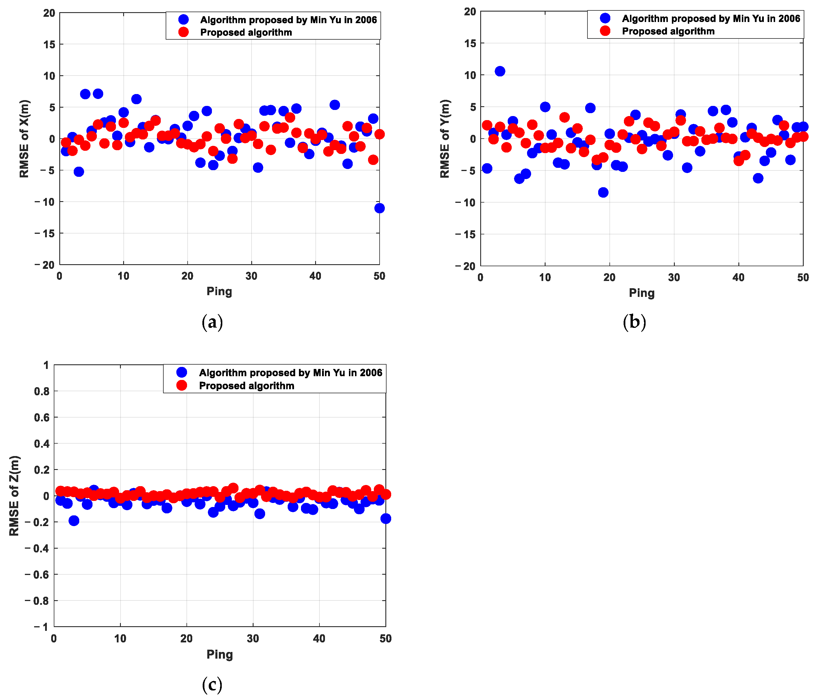
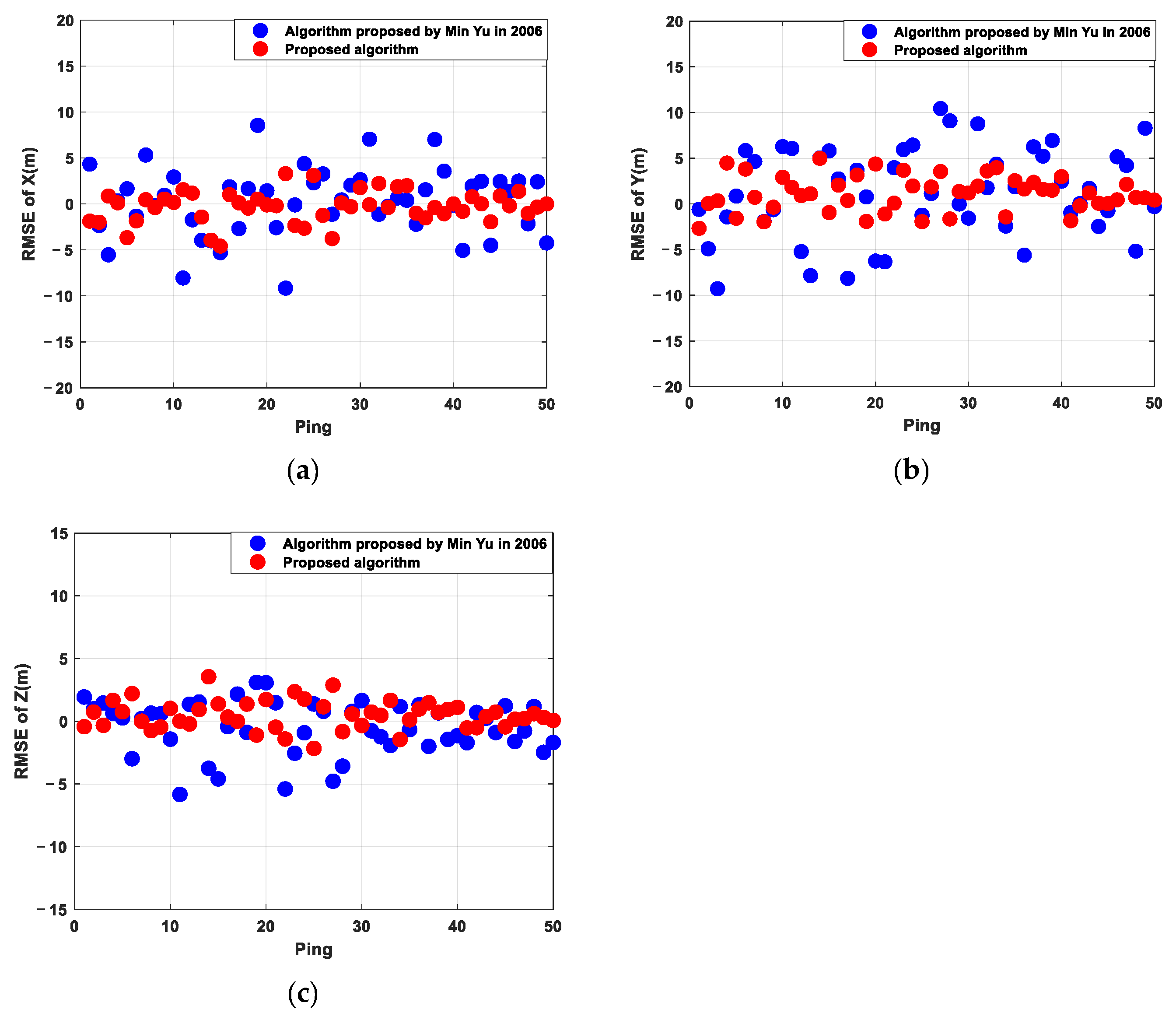
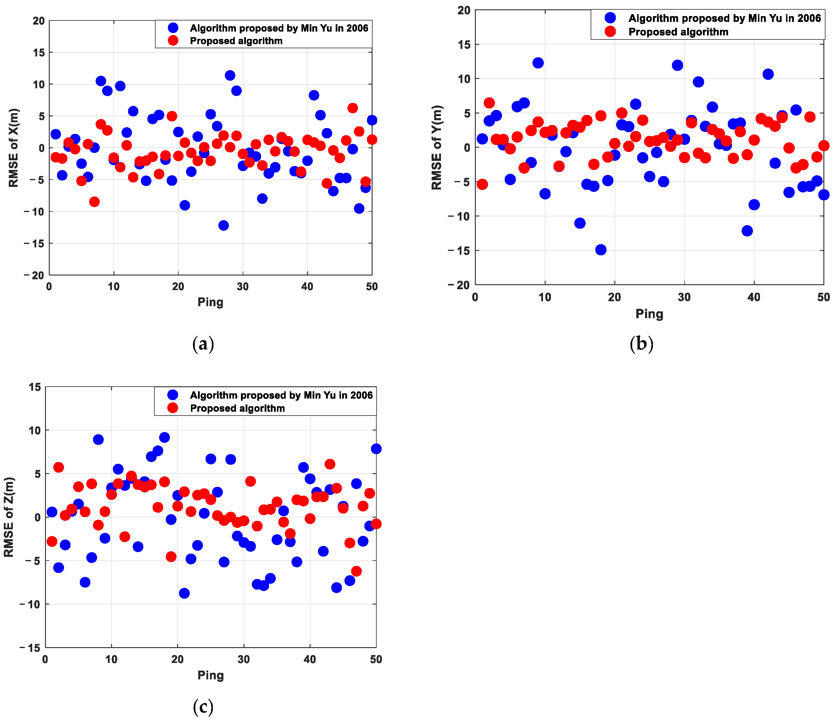
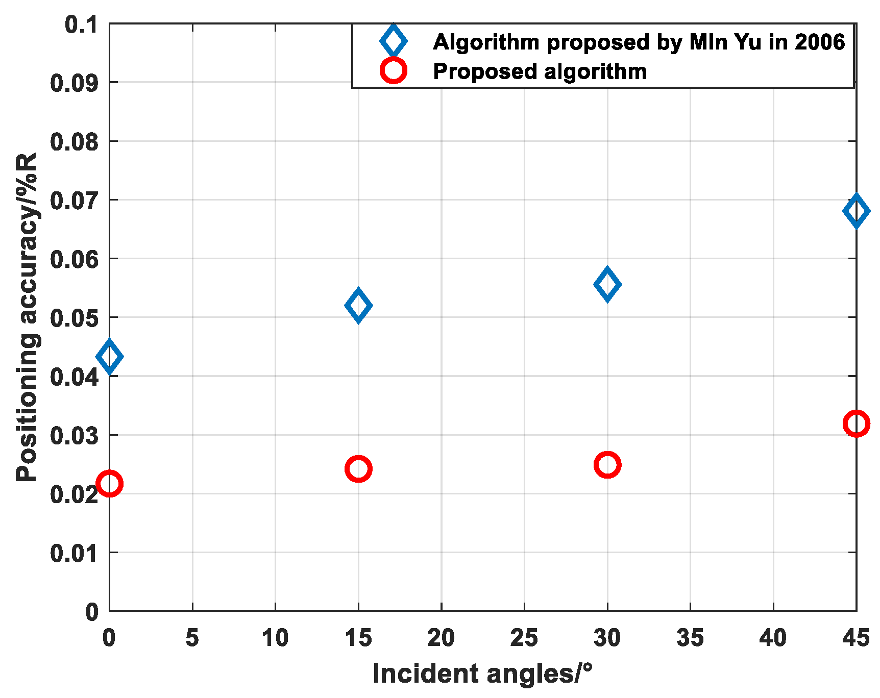
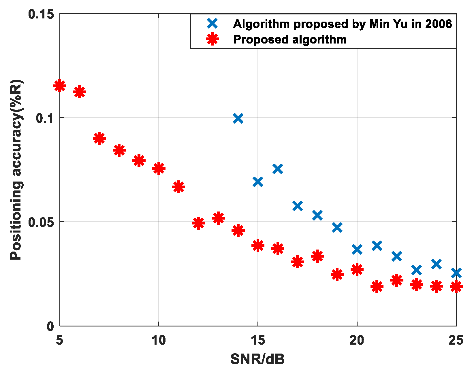
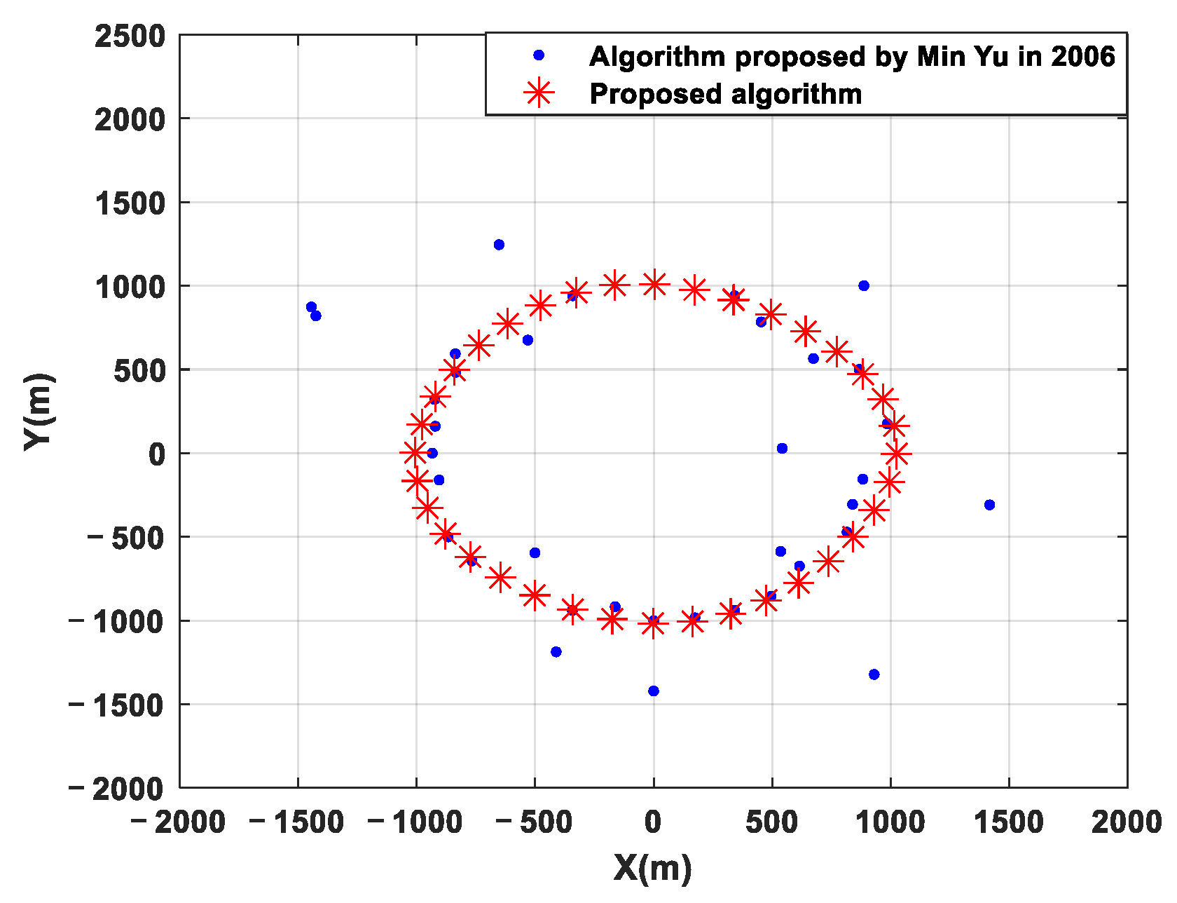
3.1. Simulation Verification

The simulation employs a synchronous mode. The time difference of synchronous trigger signal between transmitting and receiving end and the time difference of acoustic signal transmitting response trigger signal are not considered. The first two dimensions of the source coordinate represent the horizontal relative position of the source in relation to the receiving end, and the third dimension indicates the relative depth.

(1) Test 1—impact of the incident angle on localization accuracy: Four incident angles of the vertical normal between the source and the receiver array were chosen as 0°, 15°, 30°, and 45°. Fifty Monte Carlo experiments were conducted at each angle, and the simulation signal-to-noise ratio was 17 dB. The simulation results are shown in Figure 5, Figure 6, Figure 7, Figure 8 and Figure 9.

The statistical results are shown in

Table 1. Positioning accuracy.

Source Coordinates	Algorithm	RMSE (m)			Positioning Accuracy (%R)
		X-Axis	Y-Axis	Z-Axis
(−100, 80, −11,000)	Algorithm in reference [11]	3.4824	3.5471	0.0661	0.0433
	Proposed algorithm	1.5315	1.5791	0.0230	0.0217
(−2084, 2084, −11,000)	Algorithm in reference [11]	3.5373	4.5790	1.1139	0.0520
	Proposed algorithm	1.5583	1.8699	0.4373	0.0242
(−4490, 4490, −11,000)	Algorithm in reference [11]	3.6624	5.0260	2.1624	0.0556
	Proposed algorithm	1.7012	2.1838	1.1896	0.0249
(−7778, 7778, −11,000)	Algorithm in reference [11]	5.4217	5.9891	5.0455	0.0681
	Proposed algorithm	2.7301	2.7086	2.7184	0.0319

. From the simulation results, it can be seen that the positioning error gradually increases with the increase in the open angle between the sound source and the receiving array, which is consistent with the algorithm. The algorithm proposed in reference [11] achieves a maximum positioning accuracy of 0.041% R when the incident angle is 0°, and 0.0585% R when the elevation angle is ±45°. The algorithm proposed in this paper achieves a maximum positioning accuracy of 0.0243% R when the incident angle is 0°, and 0.037% R when the incident angle is ±45°. In comparison with the algorithm proposed in reference [11], the overall positioning accuracy of the algorithm proposed in this paper is superior.

(2) Test 2—Impact of the signal-to-noise ratio on localization accuracy: The source location was selected (−7778, 7778, −11,000) and 50 Monte Carlo experiments were conducted with SNR ranging from 5 dB to 25 dB for each signal-to-noise ratio. The positioning accuracy in [11] and the algorithm proposed in this paper is shown in Figure 10.

From the above simulation results, it can be seen that when the signal-to-noise ratio is greater than 13 dB, as the signal-to-noise ratio increases, the positioning accuracy of the algorithm in reference [11] and the algorithm in this paper gradually improves. In Figure 10, the positioning accuracy of the algorithm in reference [11] is not shown when the signal-to-noise ratio is lower than 13 dB, as it is excessively poor. Overall, the positioning accuracy of the algorithm in this article is better than that of the algorithm in reference [11].

(3) Test 3—Positioning stability: A circle with a depth of 1000 m and a radius of 1000 m centered on the origin was selected, with an angle step of 10°, and the signal-to-noise ratio was set as 12–13 dB. The simulation results are shown in Figure 11, Figure 12, Figure 13 and Figure 14.

From the above simulation results, it can be seen that there is a jump in the calculation of phase difference in reference [11], which is mainly due to an error in the calculation of fuzzy numbers. When the noise is high, the phase difference error of small aperture elements is considerable, which subsequently influences the ambiguity of the phase difference of large aperture elements, resulting in jumps in the positioning results. The positioning results of the algorithm presented in this article will not suffer from the issue of jumping positioning results.

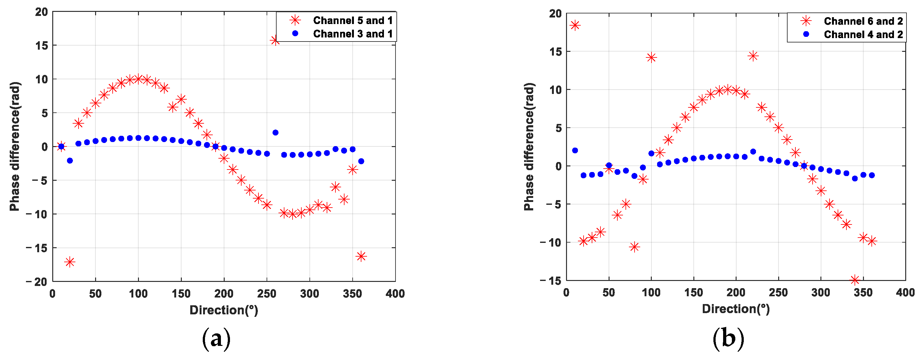
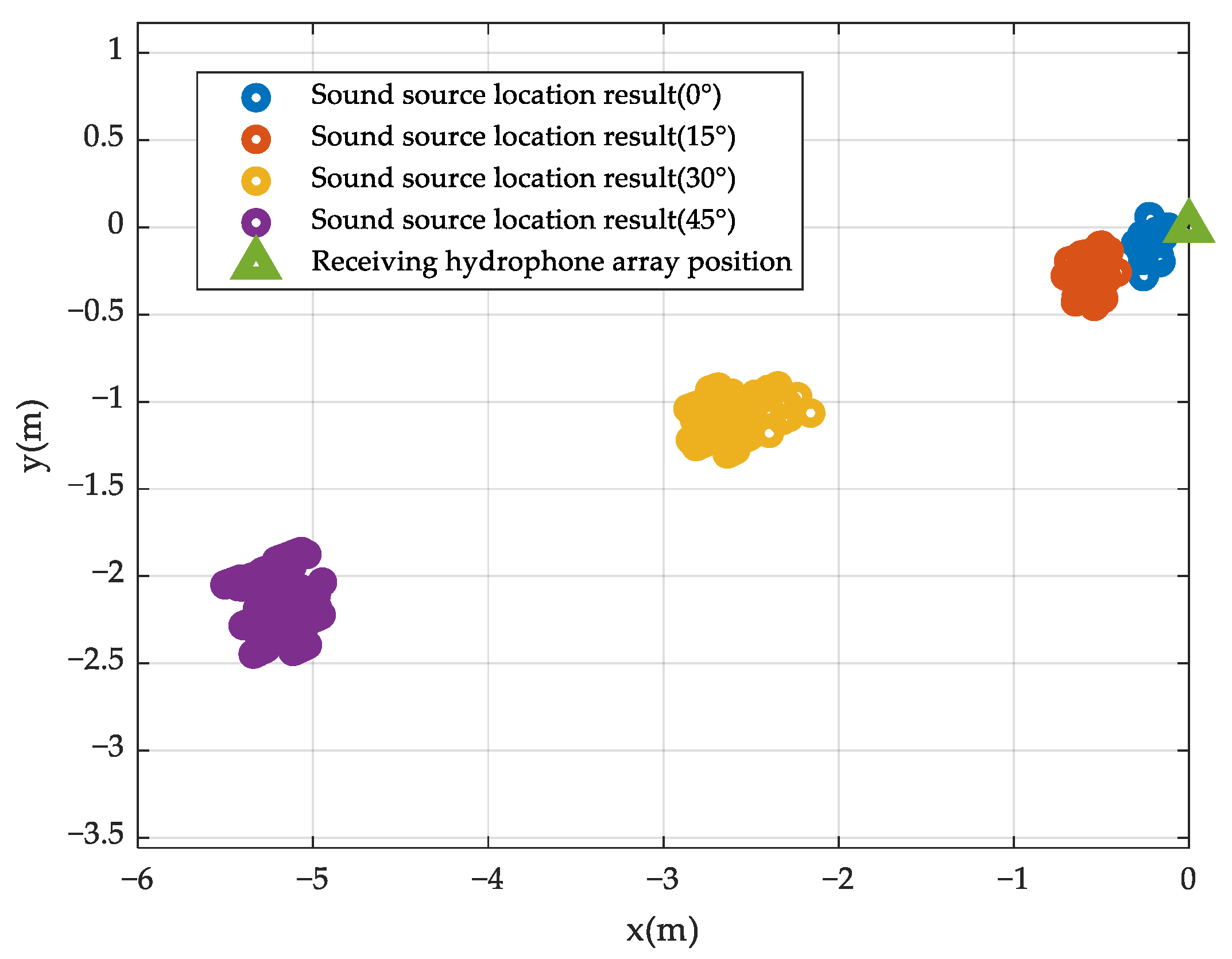
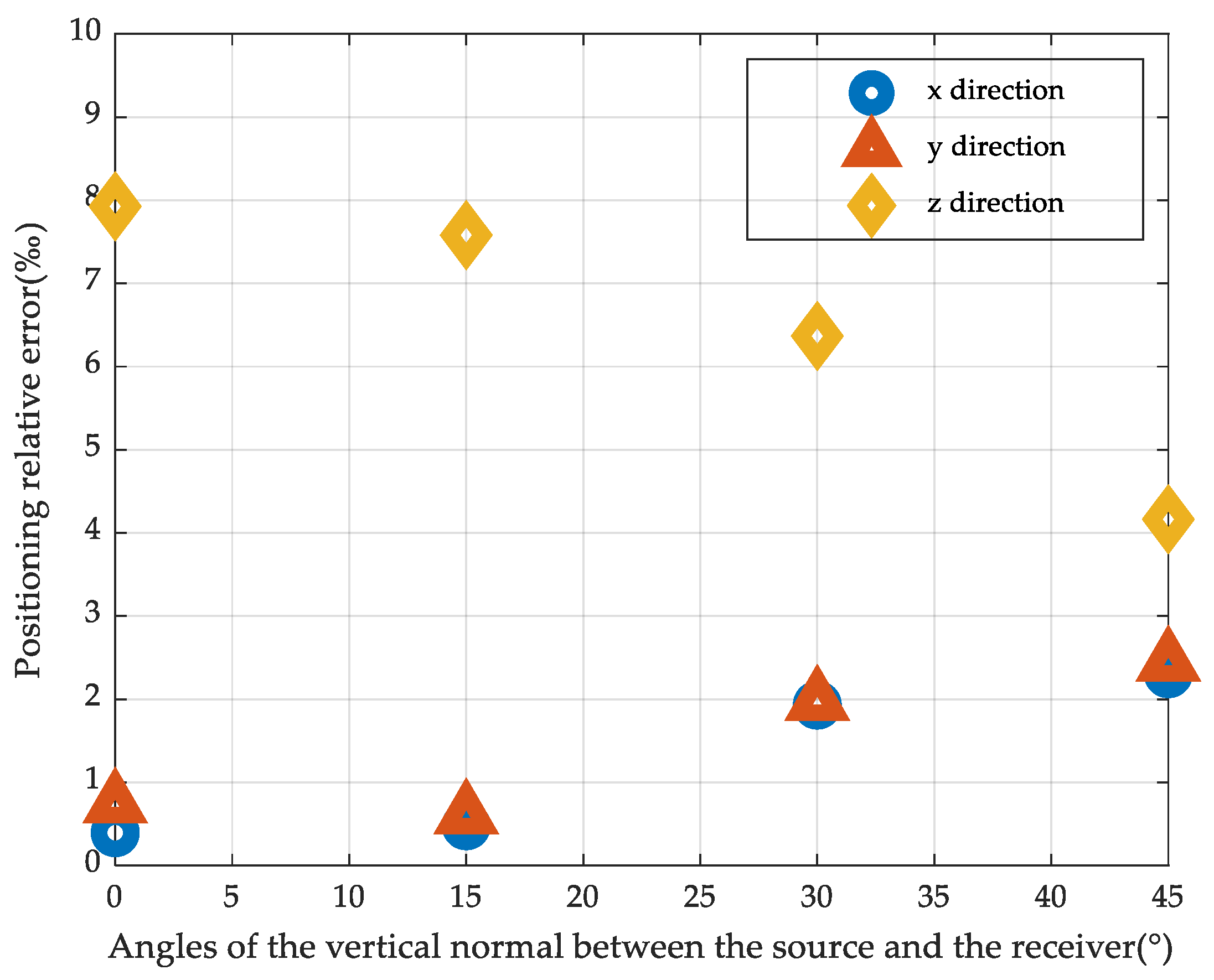
3.2. Anechoic Pool Experiment Verification

The hydrophone base array employed in this study is shown in Figure 15. Figure 15a shows the entire hydrophone base array obtained in the laboratory, while Figure 15b shows a photograph captured after the hydrophone base array has been deployed at the pond experiment site. The hydrophone array is rigidly fixed on the platform, through which the array is lowered into the water to a depth of 6 m, and the pitch angle is adjusted by altering the position of the sound source. The positioning signals are collected 100 times at the pitch angle of 0°, 15°, 30° and 45°, the positioning result is solved, and the positioning accuracy is calculated.

When the pitch angle is 0°, 15°, 30° and 45°, the positioning results are shown in Figure 16, and the average positioning error of the positioning results is shown in Figure 17. As can be seen from Figure 16, the overall positioning error can be controlled within 8‰.

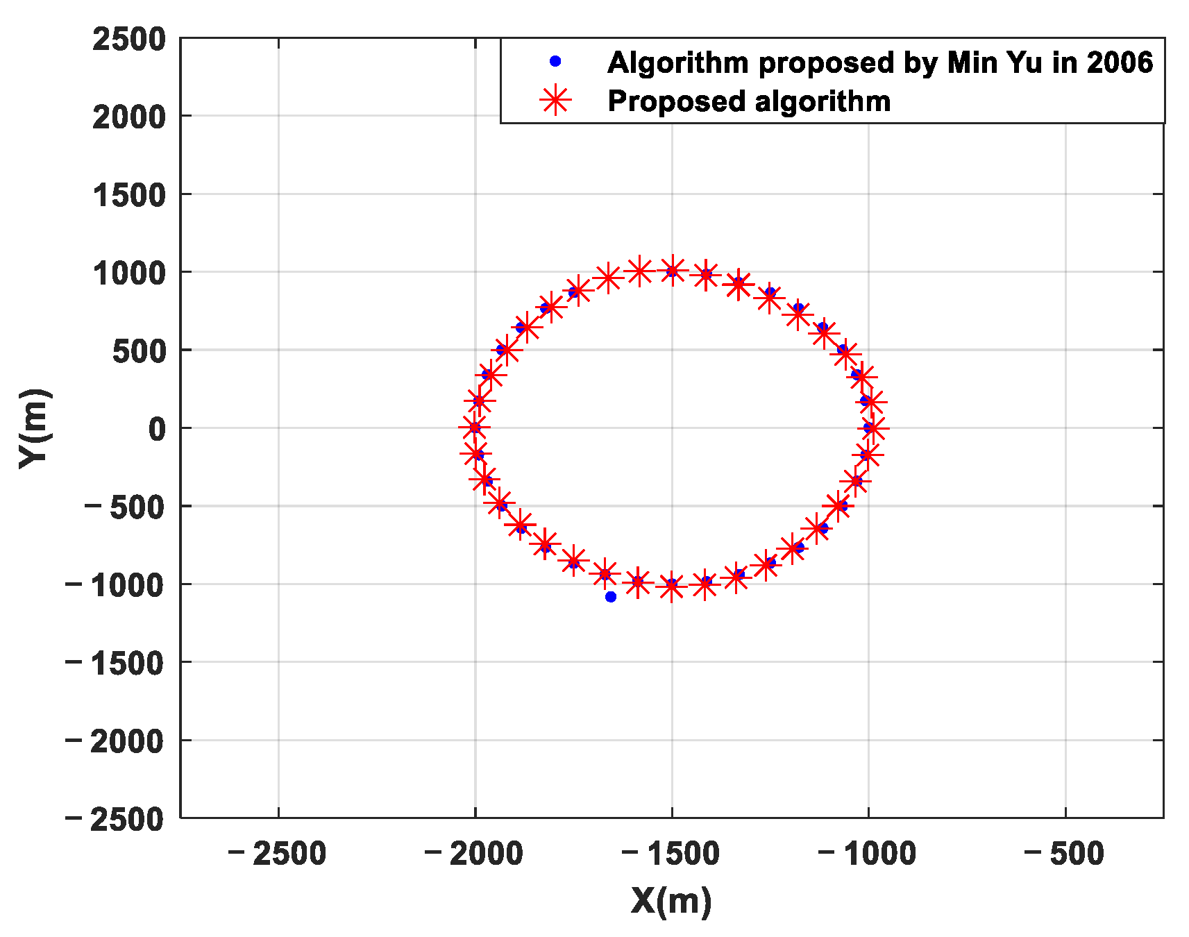
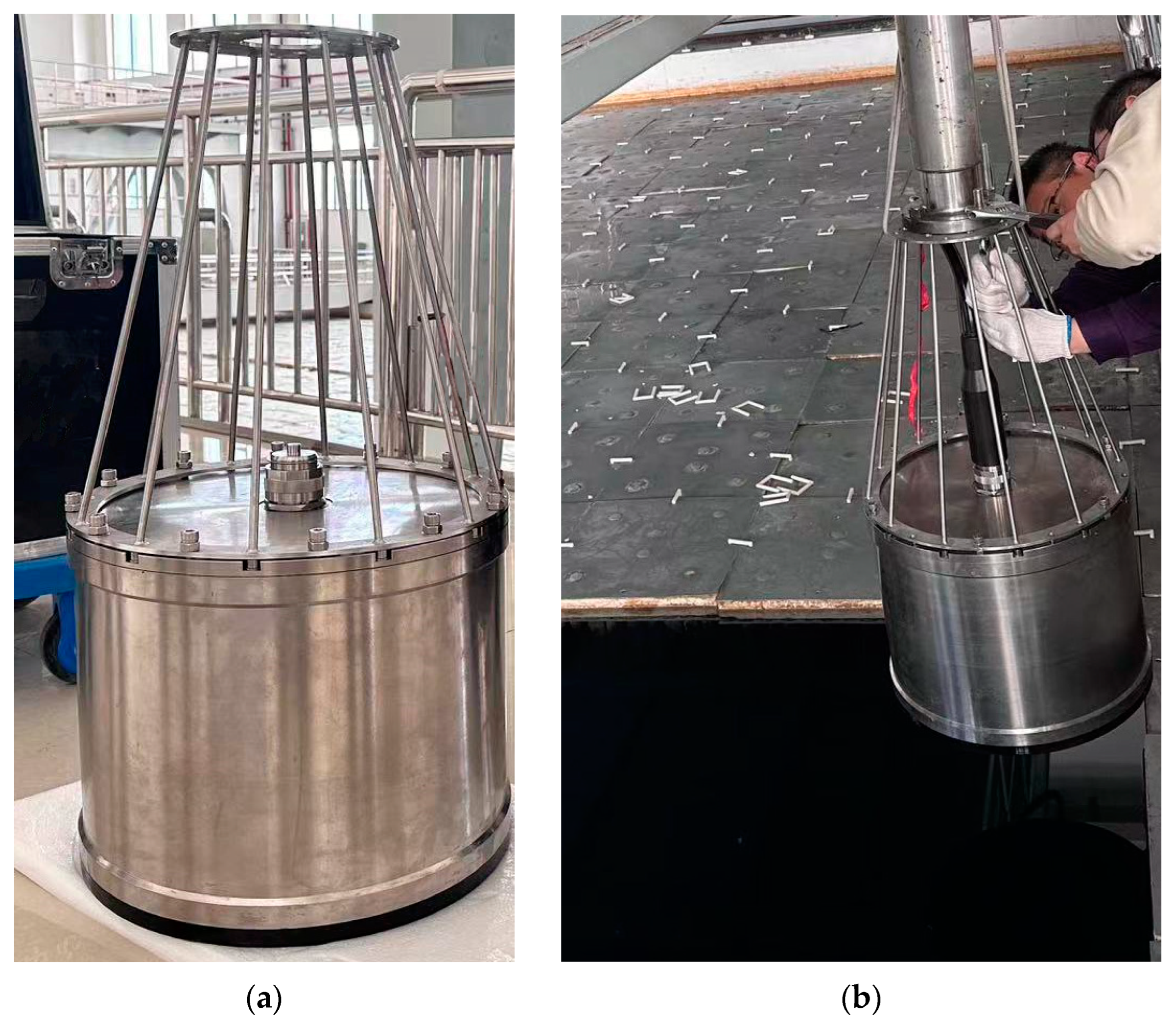
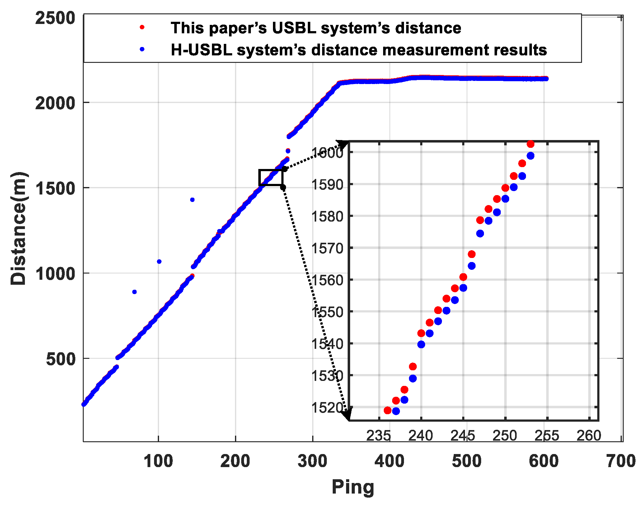
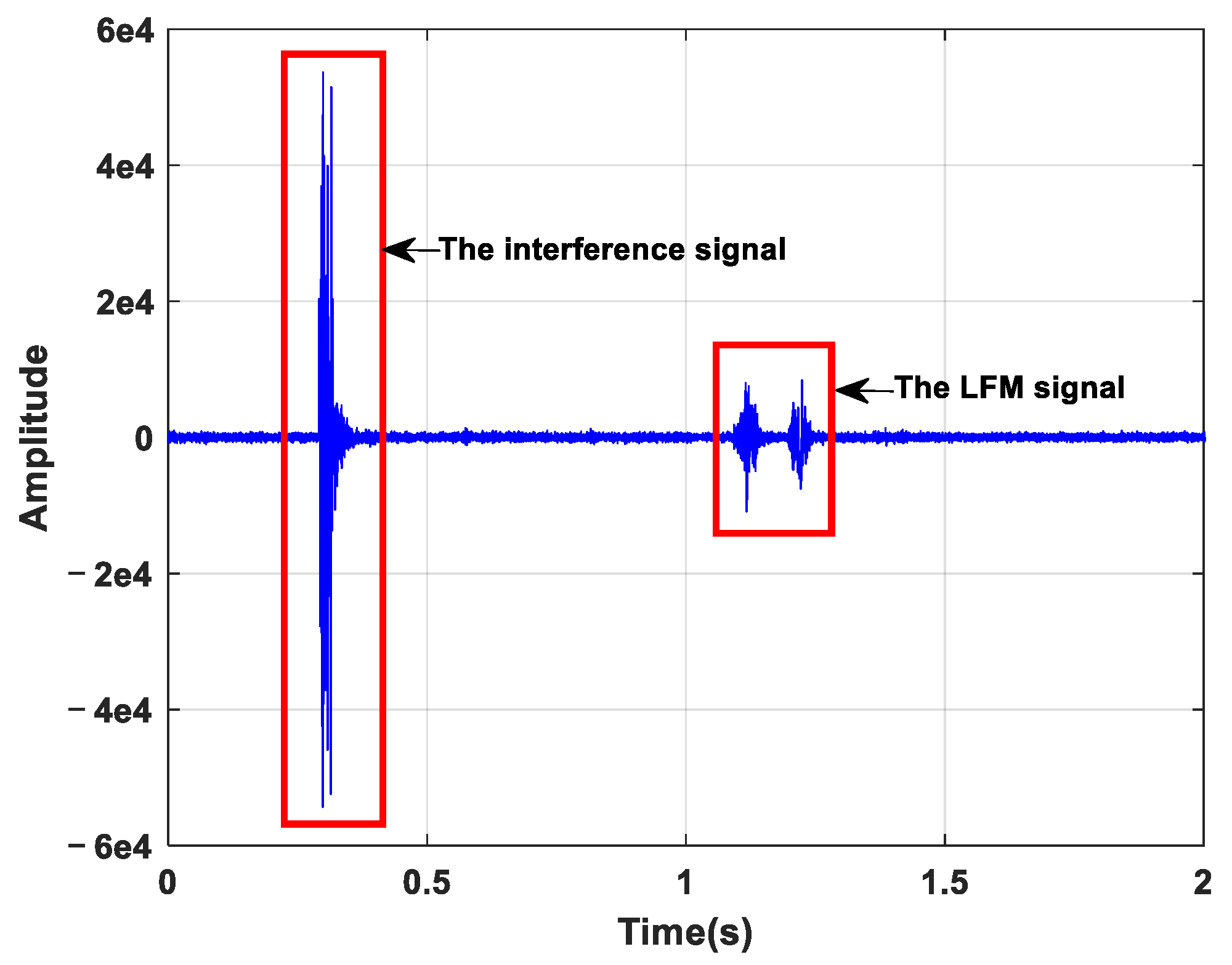
3.3. Marine Experimental Verification

The hydrophone array utilized in this paper is firmly fixed on the supporting vessel, as shown in Figure 18. The test was verified in a sea area with a depth of about 2000 m.

In order to verify the efficacy of the ultra-short baseline positioning system developed in this article, the ultra-short baseline (H-USBL) positioning system of Harbin Engineering University was chosen as a reference for the results.

The positioning array employed in this paper and the positioning array of Harbin Engineering University were utilized to locate the submerged vehicle, and the ranging results and positioning results obtained by comparison are shown in Figure 19 and Figure 20. It can be seen from Figure 19 and Figure 20 that the positioning results of the positioning array employed in this paper fit the positioning results of the positioning array of Harbin Engineering University with few wild points, which proves the effectiveness of the proposed method.

In order to verify the stability of the algorithm in this article and reduce the strength of the sound source signal in this system, the signal from Harbin Engineering was stronger than that of this system. The collected baseband signal is shown in Figure 21, Figure 22 and Figure 23.

It can be seen that the correlation amplitude of the interference signal has exceeded that of the LFM signal. In this way, if the position of the signal is only determined by the signal-to-noise ratio of the correlation results, it is prone to find the wrong position of the signal. From the correlation coefficient results, it can be seen that the output of the LFM signal is more than twice that of the interference signal, and the signal position can be accurately found through the correlation coefficient.

4. Conclusions

In response to the demand for high-precision underwater acoustic positioning at full sea depth, this paper designs a 6 * 6 square array and proposes a positioning algorithm based on the LS-ESPRIT algorithm, which integrates beam tracking and beamforming to estimate the direction of arrival. This method enables the ultra-short baseline positioning system to possess a long operating distance, high positioning accuracy, and avoid phase ambiguity. The simulation results demonstrate that the algorithm proposed in this paper has higher positioning accuracy compared to the algorithm in reference [11], with no phase ambiguity. It exhibits excellent positioning performance under a low signal-to-noise ratio, and the positioning accuracy attains 0.11% R when the signal-to-noise ratio is 5 dB. The pool and sea tests have demonstrated that the proposed method theoretically achieves high positioning accuracy within an open angle of ±45°.

In subsequent work, we shall investigate the impact of array element installation position deviation, sound velocity profile, attitude sensor installation deviation, etc., on positioning accuracy.

References

1. Liu, F. Technical Status and Development Trend of the Deep-sea Manned Submersible. J. Eng. Stud. 2016, 8, 172–178. [Google Scholar] [CrossRef]
2. Yang, B.; Liu, Y.; Liao, J. Manned Submersibles-Deep-sea Scientific Research and Exploitation of Marine Resources. Bull. Chin. Acad. Sci. 2021, 36, 622–631. [Google Scholar]
3. Ren, Y.; Liu, B.; Ding, Z. Research on the Current Status and Development Trend of Manned Submersibles. J. Ocean Technol. 2018, 37, 114–122. [Google Scholar]
4. Xu, W.; Zhang, Q. Overview of Present Status and Development Trend of Full Ocean Depth Submarines. Shipbuild. China 2016, 57, 206–221. [Google Scholar]
5. Sun, D.; Zheng, C.; Zhang, J.; Han, Y.F.; Cui, H.Y. Development and Prospect for Underwater Acoustic Positioning and Navigation Technology. Bull. Chin. Acad. Sci. 2019, 34, 331–338. [Google Scholar]
6. Liu, S.; Guo, H.; Qian, Z.; Li, J.; Wang, X.; Sun, W.; Zhang, L.; Zhang, A. A Study on a Novel Inverted Ultra-Short Baseline Positioning System and Phase Difference Estimation. J. Mar. Sci. Engs. 2003, 11, 952. [Google Scholar] [CrossRef]
7. Shi, Y.; Yin, J.; Han, X.; Guo, L. Advances in integrated technology of underwater acoustic communication, navigation, and positioning of submarines. J. Harbin Eng. Univ. 2023, 44, 1–10. [Google Scholar]
8. Sun, D.; Ding, J.; Zheng, C.; Huang, W. An Underwater Acoustic Positioning Algorithm for Compact Arrays with Arbitrary Configuration. IEEE J. Sel. Top. Signal Process. 2019, 13, 120–130. [Google Scholar] [CrossRef]
9. Wang, W.; Zhu, M.; Yang, B. Two High-Precision Ultrashort Baseline Location Methods Based on Phase Difference. IEEE Trans. Instrum. Meas. 2023, 72, 1–12. [Google Scholar] [CrossRef]
10. Sun, D.; Cai, H.; Zheng, C.; Cheng, C. Stereo Array Positioning Algorithm Based on Vector Projection. J. Electron. Inf. Technol. 2022, 45, 31–40. [Google Scholar]
11. Yu, M.; Hui, J.; Feng, H.; Zhang, X. Improved measurement methods for positioning precision of USBL. Ocean Eng. 2006, 24, 86–91. [Google Scholar]
12. Zheng, C.; Li, Q.; Sun, D.; Zhang, D. An Improved Measurement Method for Array Design of USBL. Period. Ocean Univ. China 2009, 39, 505–508. [Google Scholar]
13. Zheng, E.; Chen, X.; Sun, C.; Yu, H. An innovation four-element array to achieve high-precision positioning of the Ultra-short baseline. Appl. Acoust. 2013, 32, 15–22. [Google Scholar]
14. Luo, Q.; Yan, X.; Ju, C.; Chen, Y.; Luo, Z. An Ultra-Short Baseline Underwater Positioning System with Kalman Filtering. Sensors 2021, 21, 143. [Google Scholar] [CrossRef] [PubMed]
15. Zhu, Y.; Luo, J.; Zhang, K. DOA Estimation Algorithm of Wideband Digital Signal Based on Fitting Phase Difference and Frequency. Mod. Def. Technol. 2013, 41, 131–135. [Google Scholar]
16. Debasis, K. Modified MUSIC algorithm for estimating DOA of signals. Signal Process. 1996, 48, 85–90. [Google Scholar]
17. Viberg, M.; Ottersten, B.; Kailth, T. Detection and estimation in sensors arrays using weighed subspace fitting. IEEE Trans. Signal Process. 1991, 39, 2436–2449. [Google Scholar] [CrossRef]
18. Viberg, M.; Ottersten, B. Sensor array processing based on subspace fitting. IEEE Trans. Signal Process. 1991, 39, 1110–1121. [Google Scholar] [CrossRef]
19. Richard, R.; Thomas, K. ESPRIT-Estimation of Signal Parameters Via Rotational Invariance Techniques. IEEE Trans. Acoust. Speech Signal Process. 1989, 37, 984–995. [Google Scholar]
20. Zhu, F.-Y.; Chai, S.-R.; Zou, Y.-F.; He, Z.X.; Guo, L.X. An Efficient and Accurate RCS Reconstruction Technique Using Adaptive TLS-ESPRIT Algorithm. IEEE Antennas Wirel. Propag. Lett. 2024, 23, 49–53. [Google Scholar] [CrossRef]
21. Tian, T. Sonar Technology; Harbin Engineering University Press: Harbin, China, 2009; pp. 87–88. [Google Scholar]
22. Zheng, J.; Ying, Q.; Yang, W. Signal and System; Higher Education Press: Beijing, China, 2000; pp. 341–346. [Google Scholar]
23. Jia, W. The Calculation Method of the Eigenvalues of the Matrix. J. Dezhou Univ. 2017, 33, 1–8. [Google Scholar]
24. Zhang, X.; Zhang, Y. Research on the Calibration Method of the Array Installation Error in Ultra-short Baseline Underwater Acoustic Locating System. Mine Warf. Ship Self-Def. 2012, 20, 28–31. [Google Scholar]
25. Li, H.; Han, Y.; Zheng, C. Application of sound speed correlation technology in highly precise underwater positioning system. J. Navig. Position. 2020, 8, 47–52. [Google Scholar]
26. Yu, M.; Cai, K.; Zheng, C.; Sun, D. Improvement of seafloor positioning through correction of sound speed profile temporal variation. IEEE/CAA J. Autom. Sin. 2023, 10, 2023. [Google Scholar] [CrossRef]
Figure 1. System components.
Jmse 12 01689 g001
Figure 2. Receiving hydrophone array diagram. The black and blue dots represent hydrophones, while the black dots also represent the origin position of the coordinates.
Jmse 12 01689 g002
Figure 3. Quadrature demodulation.
Jmse 12 01689 g003
Figure 4. Array decomposition.
Jmse 12 01689 g004
Figure 5. RMSE at 0° incident angle. (a) X-axis, (b) Y-axis, (c) Z-axis [11].
Jmse 12 01689 g005
Figure 6. RMSE at 15° incident angle. (a) X-axis, (b) Y-axis, (c) Z-axis [11].
Jmse 12 01689 g006
Figure 7. RMSE at 30° incident angle. (a) X-axis, (b) Y-axis, (c) Z-axis [11].
Jmse 12 01689 g007
Figure 8. RMSE at 45° incident angle. (a) X-axis, (b) Y-axis, (c) Z-axis [11].
Jmse 12 01689 g008
Figure 9. Positioning accuracy at different incident angles [11].
Jmse 12 01689 g009
Figure 10. Positioning accuracy at different SNR [11].
Jmse 12 01689 g010
Figure 11. Positioning result of SNR at 12 dB [11].
Jmse 12 01689 g011
Figure 12. Phase difference of SNR at 12 dB. (a) Channel 5 and 1, Channel 3 and 1; (b) Channel 6 and 2, Channel 4 and 2.
Jmse 12 01689 g012
Figure 13. Positioning result of SNR at 13 dB [11].
Jmse 12 01689 g013
Figure 14. Phase difference of SNR at 13 dB. (a) Channel 5 and 1, Channel 3 and 1; (b) Channel 6 and 2, Channel 4 and 2.
Jmse 12 01689 g014
Figure 15. Anechoic pool experiment. (a) Hydrophone array diagram; (b) Installation of hydrophone array in pool.
Jmse 12 01689 g015
Figure 16. Anechoic pool experiment: schematic diagram of position results.
Jmse 12 01689 g016
Figure 17. Anechoic pool experiment: position error diagram.
Jmse 12 01689 g017
Figure 18. Installation diagram of a hydrophone array supporting a ship.
Jmse 12 01689 g018
Figure 19. Distance measurement comparison diagram.
Jmse 12 01689 g019
Figure 20. Comparison diagram of carrier coordinate systems’ positioning results.
Jmse 12 01689 g020
Figure 21. The collected baseband signal.
Jmse 12 01689 g021
Figure 22. The correlation result.
Jmse 12 01689 g022
Figure 23. The correlation coefficient result.
Jmse 12 01689 g023