Numerical Simulation of Subaerial Granular Landslide Impulse Waves and Their Behaviour on a Slope Using a Coupled Smoothed Particle Hydrodynamics–Discrete Element Method

Abstract

Numerical simulations were conducted to investigate the wave features of subaerial granular landslide-generated impulse waves and their impact on slopes. A numerical solution was obtained by coupling smoothed particle hydrodynamics (SPH) and the discrete element method (DEM). Several predictive equations were tested for their applicability in predicting the maximum crest amplitude of impulse waves generated by slides of different shapes. The results indicated that the predictive model developed by Heller and Hager, utilising slide centroid impact velocity, showed favourable prediction accuracy for the maximum crest amplitude, almost independent of the slide shape at impact. Regarding the leading wave, although the wave profile and velocity distribution deviated significantly from a solitary wave of the same wave amplitude, the maximum run-up could be satisfactorily estimated using solitary wave theory. In addition, the increase in the maximum dynamic forces exerted by the impulse waves on the slope followed a power law with the incident wave amplitude.

1. Introduction

In channel reservoirs, rapid increases or decreases in water levels can influence the stability of the surrounding slopes, potentially triggering landslides; for example, the Gongjiafang landslide occurred during a 175 m trial impounding in the Three Gorges Reservoir, China [1]. Landslides can impact a water body at extremely high speeds, resulting in high-energy impulse waves. Impulse waves can impose violent loads on ships and even prevent navigation in channel reservoirs [2]. Furthermore, such waves may interact intensely with downstream structures (e.g., dams, weirs, or gates), which may cause structural damage and possibly compromise their stability [3,4,5]. In addition, impulse waves that surge up the opposite slope can result in significant losses of life and property [6].

The reliable prediction of the wave characteristics of landslide impulse waves is essential for evaluating the potential damage caused by such natural hazards. Subaerial landslide impulse waves, in particular, pose significant challenges due to the complex interactions between the sliding mass and the water body, often accompanied by substantial air entrainment [7]. Numerous investigations have been conducted to predict wave behaviour by schematising subaerial landslides as rigid blocks [8,9,10,11,12,13] or a cluster of granular material [14,15,16,17,18,19,20,21]. In nature, subaerial landslides are typically composed of a mixture of large and small blocks and clusters of gravel and sand [19]; thus, their shapes can be very different in terms of impact, owing to the complex deformation mechanism incurred during rundown. Several studies have considered the block shape effect on impulse wave features [9,22]. In contrast, the influence of the granular slide shape on impulse waves has received comparatively less attention. Moreover, the slide Froude number, calculated using the characteristic slide velocity, is considered the dominant dimensionless parameter for impulse wave feature prediction, for example, the maximum wave amplitude. However, the selection of slide characteristic velocities has not been unified for impulse waves generated by granular slides, mainly including slide centroid velocity at impact [15] and slide centroid impact velocity [7]. This inconsistency in parameter selection complicates the prediction of wave characteristics.

The main objective of this study is to investigate the characteristics of impulse waves generated by subaerial landslides with different slide shapes at impact and identify the key characteristic slide velocity for wave feature prediction. The SPH-DEM coupling method offers distinct advantages over other techniques in simulating the process of landslide-generated waves. Its combination of the Lagrangian SPH method, which efficiently models free-surface flows with breaking and splash, and the DEM, which excels in simulating the granular flows of solid particles, provides a robust framework for analysing the complex dynamics of landslides involving both fluid and granular components. This approach effectively addresses the challenges of large deformations, post-failure movements, and complicated solid–fluid coupling problems, making it particularly suitable for simulating the intricate process of landslide-induced wave generation. Thus, a numerical flume model based on the coupled smoothed particle hydrodynamics (SPH)–discrete element method (DEM) was constructed. In the model, the parameters governing the solid–water coupling process were selected to produce slides with different shapes upon impact. Several well-known predictive equations were evaluated for their effectiveness in predicting the maximum crest amplitude with different characteristic slide velocities as the input parameters. In addition, the maximum run-up height on the slope and the dynamic wave force exerted by the impulse wave on the slope were analysed.

2. Numerical Simulation

2.1. Establishment of Numerical Model

A schematic of the two-dimensional numerical model is shown in Figure 1. The model is equipped with two inclined planes: the upstream plane with an adjustable angle α was used for sliding granular materials, whereas the downstream plane with a constant slope angle β = 45° was set up to investigate the behaviour of landslide-generated surges. A horizontal channel length of 2.5 m was used to connect the two planes. The height of the computational domain was set to 2.5 m. Thus, the total length of the domain was dependent on the slope angle α. In this study, solid aluminium cylinders piled up as several layers were used to simulate a granular slide. The initial shape in the vertical plane was rectangular, with a length of l_s0 and a thickness of s₀.

Two different coordinate systems were used in this study: the o’ξ coordinate system for describing the centre position of slides during rundown and the oxz coordinate system for depicting wave features in the channel. Note that origin o’ refers to the intersection of the upstream slope and the still water surface, whereas origin o is defined at the base of the downstream slope at the start of the channel.

2.2. Simulation Conditions

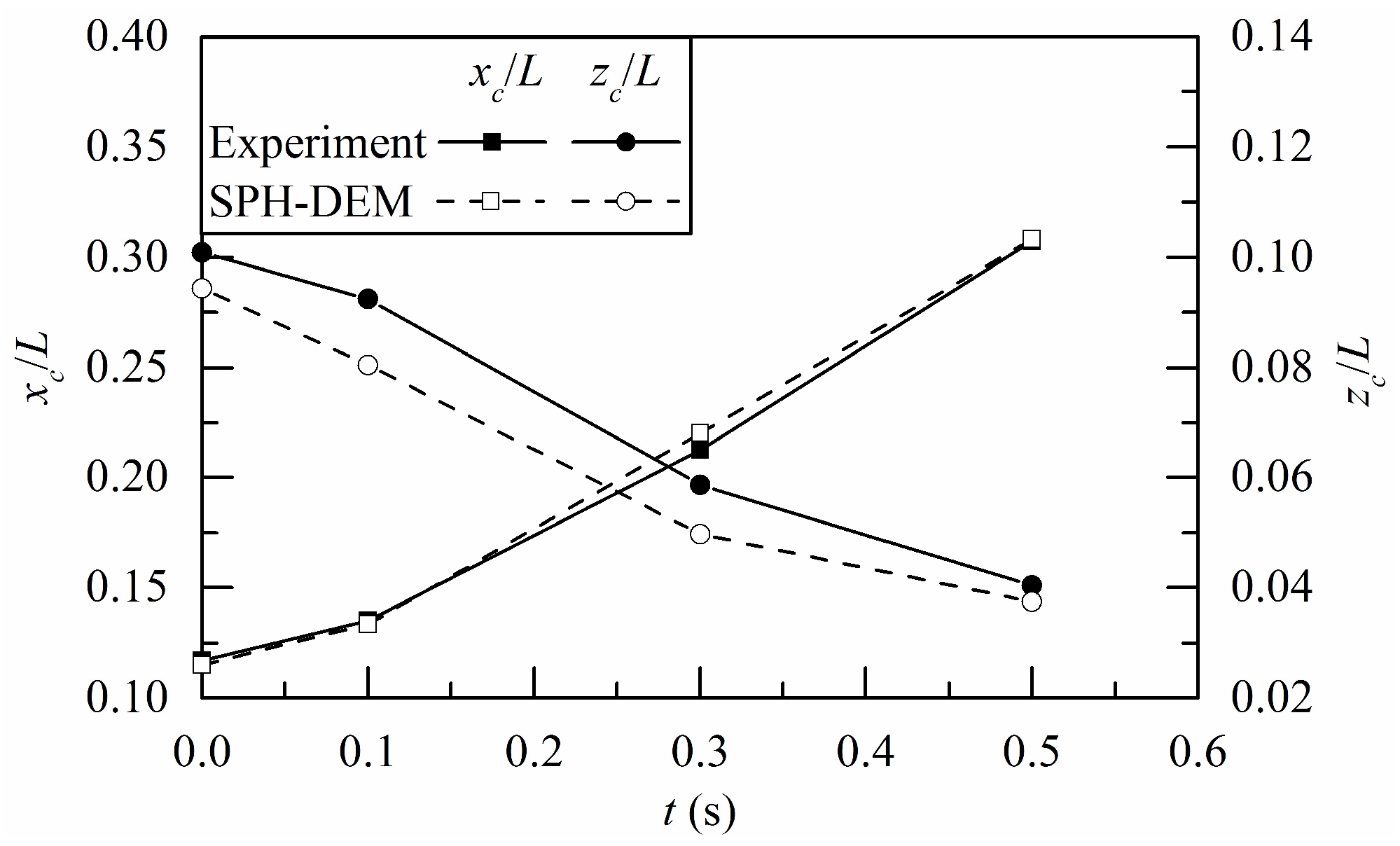
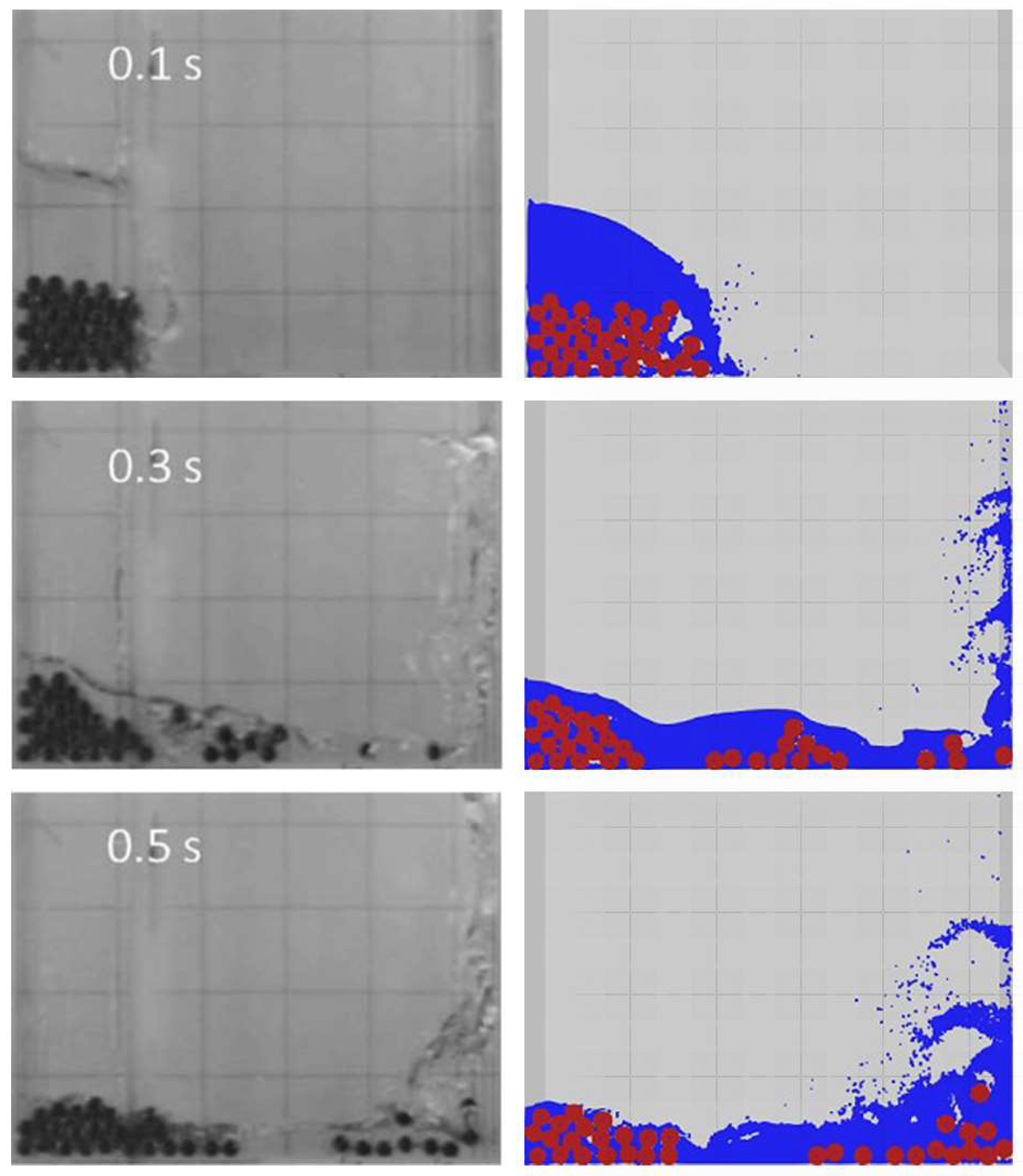
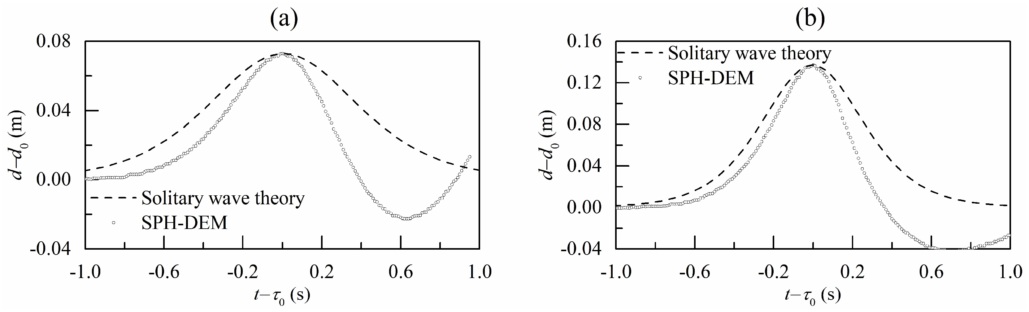
The mechanisms governing the wave generation process are related to many factors, which can be grouped into three categories: (a) slide static parameters, such as slide mass m_s, bulk slide volume V_s, grain density ρ_g, and grain diameter d_g; (b) slide dynamic parameters, such as slide impact shape, slide impact thickness s, and slide characteristic velocity at impact; (c) configuration parameters, including slope angle α and still water depth d₀.

To ensure the accuracy and reliability of the numerical calculation, the density ρ_g and diameter d_g of the solid cylinders were set to 2700 kg/m³ and 0.01 m, respectively, consistent with the verification conditions of the SPH-DEM coupling model presented later. Five parameters were selected and combined to study the impulse wave characteristics: slide length l_s0, thickness s₀ before slide release, slide drop height h_0c, slide impact angle α, and still water depth d₀. The variation in the slide volume V_s or mass m_s was controlled by the variation in l_s0 or s₀, while the variations in the slide dynamic parameters, dependent on the combination of the five governing parameters, were not considered indirectly. Four values were tested for each parameter, and they were selected to produce slides with different shapes upon impact. The main details of the numerical simulations based on orthogonal design are listed in

Table 1. Details of simulations.

Case	α (°)	d0 (m)	hc0 (m)	ls0 (m)	s0 (m)	Slide Shape Type	Vsc0 (ms−1)	Vsc1 (ms−1)	S	M
R1	30	0.2	0.3	0.2	0.10	B	0.96	1.22	0.364	1.060
R2	30	0.4	0.6	0.4	0.20	B	1.16	1.57	0.343	1.060
R3	30	0.6	0.9	0.5	0.25	B	1.39	1.81	0.197	0.736
R4	30	0.8	1.2	0.6	0.30	B	1.51	1.95	0.177	0.596
R5	40	0.2	0.6	0.5	0.30	B	1.35	2.18	1.054	7.952
R6	40	0.4	0.3	0.6	0.25	A	0.42	1.75	0.574	1.988
R7	40	0.6	1.2	0.2	0.20	C	2.17	2.71	0.130	0.236
R8	40	0.8	0.9	0.4	0.10	C	2.00	2.55	0.111	0.133
R9	50	0.2	0.9	0.6	0.20	B	2.12	3.14	0.853	6.362
R10	50	0.4	1.2	0.5	0.10	C	2.77	3.49	0.248	0.663
R11	50	0.6	0.3	0.4	0.30	A	0.77	1.89	0.450	0.707
R12	50	0.8	0.6	0.2	0.25	B	1.82	2.46	0.160	0.166
R13	60	0.2	1.2	0.4	0.25	B	3.08	3.96	0.790	5.301
R14	60	0.4	0.9	0.2	0.30	B	2.64	3.28	0.364	0.795
R15	60	0.6	0.6	0.6	0.10	B	1.84	2.86	0.161	0.353
R16	60	0.8	0.3	0.5	0.20	A	0.72	2.04	0.232	0.331

.

The free-surface characteristics of landslide-generated waves in the wave-generation zone were mainly controlled by the following dimensionless parameters: slide Froude number F = V_sc/(gd₀)^1/2, with characteristic slide velocity V_sc and gravitational acceleration g; relative slide thickness S = s/d₀ (0.111 ≤ S ≤ 1.054); relative slide mass M = m_s/(ρ_wb_sd₀²), with water mass density ρ_w and slide width b_s (0.133 ≤ M ≤ 7.952); slide impact angle α (30° ≤ α ≤ 60°). In this study, the investigated values of S, M, and α were close to the test ranges of earlier studies [16,18,20]. In addition, the minimum value of the still water depth d₀ was set to 0.2 m to avoid scale effects in the wave generation process [23].

2.3. Validation

The Lagrangian method SPH offers an efficient technique for modelling free-surface flows, particularly those involving breaking and splash phenomena. On the other hand, the DEM exhibits a notable advantage in simulating granular flows composed of solid particles [24]. In the context of granular landslide-generated impulse waves, three primary interaction types are present: fluid–fluid, fluid–solid, and solid–solid interactions. In this study, these interactions were comprehensively simulated using the open-source integrated framework DualSPHysics [25], specifically the beta executable of version 5.0. This framework provides a robust coupling between the SPH and DEM methodologies. Within the DualSPHysics environment, both fluid–fluid and fluid–solid interactions were calculated using the Navier–Stokes equation and the continuity equation, leveraging the SPH method. When addressing fluid–solid interactions, the boundary encompassing solid particles was designed to additionally adhere to Newton’s equations for rigid body dynamics [26], indicating the adoption of the Dynamic Boundary Condition. In the context of floating bodies, their motion is characterised by the net force acting on each boundary particle, which is the sum of the contributions from all surrounding fluid particles. Conversely, for boundary domains, these particles remain fixed in position. The interaction between solid particles was modelled using the DEM approach. For a more detailed numerical treatment, readers may refer to the studies conducted by Canelas et al. [26,27].

Once a subaerial uniform granular slide was released, it accelerated under gravity and deformed during rundown, subsequently impacting the water body, resulting in the generation of impulse waves. Therefore, the subaerial deformation of the slide in the vertical plane may be characterised by the collapse of multiple solid cylinder layers. The interaction between the slide and water body is a complicated fluid–solid mixture flow problem. In this section, experiments conducted by Zhang et al. [28] were simulated to validate the proposed SPH-DEM model operating under the two conditions above. The first simulation involved the collapse of six solid cylinder layers, whereas the second simulation involved the breaking of a water dam with a height of 12 cm involving six solid cylinder layers submerged in water.

In the model, six solid cylinder layers were stacked in a 26 cm long, 10 cm wide, and 26 cm deep horizontal rectangular tank with a vertical gate 6 cm from its left wall. The cylinders and tank were made of aluminium and acrylic, respectively. The density and diameter of the cylinders were 2700 kg/m³ and 0.01 m, respectively. The cylinders had a uniform length of 9.9 cm. The cylinders (and water) were released by rapidly removing the gate and collapsing it by gravity. The primary parameters used in the computations are listed in

Table 2. Numerical parameters used in the simulations.

Description	Selected Value
Interaction kernel function	Wendland
Time-stepping algorithm	Symplectic
Viscosity formulation method	Laminar + Sub-particle-scale
Kinematic viscosity	10−6 m2s−1
Density filter	Delta-SPH formulation
Initial distance between particles	0.0005 m

. The material properties of the cylinders and tank were the same as those used in the simulations of Canelas et al. [27] and are presented in

Table 3. Material properties used in the simulations.

Object	Material	Young’s Modulus (Nm−2)	Poisson Ratio	Kinetic Friction Coefficient	Restitution Coefficient
Cylinders	Aluminium	69 × 109	0.30	0.45	0.886
Tank	PVC	30 × 108	0.30	0.45	0.65

.

In Figure 2, the simulated temporary behaviour of the cylinders for the collapse of the six solid cylinder layers is compared with the experimental results. The temporal variation in the average mass centre of the cylinders is shown in Figure 3, where x_c and z_c are the positions of the mass centres in the horizontal and vertical directions, respectively, and are scaled by the tank length L. The numerical and experimental results were in good agreement, and the dynamic features of the cylinder were well reproduced.

Figure 4 shows the simulation results for the mixture flow and their comparison with the test results. The movement process of the cylinders was in reasonable agreement with the test results. The numerical simulation successfully repeated the phenomenon in which most cylinders accumulated on the left side of the tank during dam breakage. Overall, the results showed that the SPH-DEM coupled model is capable of reproducing the key features of solid–fluid interactions.

3. Results and Discussion

3.1. Slide Shape

Once the granular material was released, it slid freely down the slope under the force of gravity and deformed. Figure 5 presents the typical geometries of the slides when their front reached the still water surface (t = 0 s). Overall, three slide-shape patterns—Types A, B, and C—were recognised. Type A occurred if the release position of the slide was close to the still water. The slide impacted the water surface with a nearly rectangular cross-section, with the slide front angle close to 90° (see Figure 5a). As the slide drop height between the slide release and the still water surface increased, the slide underwent significant deformation during the rundown slope, becoming semi-elliptical in shape at impact (i.e., Type B), as indicated in Figure 5b. This slide shape is consistent with the observations reported by Fritz et al. [18], Zweifel et al. [20], and Heller and Hager [16]. In this study, the slide front angle for the Type B slides ranged between 5° and 28°. A slide initially positioned farther from the still water underwent complete deformation during the slope rundown, ultimately transforming into a lengthy and slender material train with an approximately uniform mean thickness at impact (i.e., Type C), as depicted in Figure 5c. This slide type aligns with the observations documented by Miller et al. [15].

3.2. Maximum Wave Amplitude

The maximum crest amplitude plays a crucial role in hazard assessment and mitigation [18]. In this study, the leading wave in a wave group always had the maximum wave crest amplitude at locations in the wave generation zone. Miller et al. [15] stressed that, in the impact region, the submerged mass usually travels at a higher velocity than the impulse wave. In this context, the front edge of the mass was downstream of the leading wave crest, leading to a rapidly developing wave with an unstable wave profile owing to consistent energy transfer from the slide to the wave. Therefore, the maximum wave amplitude a_m referred to the wave amplitude of the leading wave at a location where the leading wave crest just exceeds the slide front.

Several equations based on the slide Froude number F, relative slide thickness S, relative slide mass M, and slide impact angle α have been developed to estimate the maximum wave amplitude of impulse waves generated by a subaerial granular mass. In a study by Fritz et al. [18], the value of a_m/d₀ is related to F and S as follows:

$$a_m/d_0=0.25F^{1.4}{S}^{0.8},$$

(1)

The experimental data of Zweifel et al. [20] led to a different relationship by considering the effect of slide density.

$$a_m/d_0=1/3F{S}^{1/2}{M}^{1/4},$$

(2)

Heller and Hager [16] evaluated the maximum wave amplitude as a function of the impulse product parameter P = FS^1/2M^1/4{cos[(6/7)α]}^1/2, resulting in the following:

$$a_m/d_0=4/9P^{4/5},$$

(3)

Notably, the selection of slide characteristic velocities used to calculate the slide Froude number has remained non-unified for the impulse waves generated by granular slides, primarily encompassing the slide centroid velocity at impact and the slide centroid impact velocity. In this study, the centre of mass in the oxz coordinate system (x_sc, z_sc) can be computed using the following equation:

$$\left\{\begin{array}{c}{x}_{sc}=1/n {\sum }_{i=1}^n{x}_i\\ z_{sc}=1/n {\sum }_{i=1}^n{z}_i\end{array},\right.$$

(4)

where n is the number of solid cylinders and (x_i, z_i) denotes the centroid position of each cylinder. The position of the mass in the coordinate system o’ξ (ξ_sc) is determined using a projection method. Subsequently, the slide centroid velocity was calculated as the temporal derivative of ξ_sc, as referenced by Lindstrøm [19]. The characteristic slide velocities—namely, the slide centroid velocity at impact (V_sc0) and the slide centroid impact velocity (V_sc1)—are listed in Table 1 for each slide.

The performance of the above predictive equations was evaluated, with both V_sc0 and V_sc1 used as input variables to assess their prediction efficiency. A comparison of the computed a_m/d₀ values obtained from the predictive equations and the numerical results is presented in Figure 6. As evident in Figure 6a, the existing maximum wave amplitude equations demonstrated generally poor performance, with significant underprediction when the slide centroid velocity at impact V_sc0 was used. However, when the slide centroid impact velocity V_sc1 was applied for a_m/d₀ predictions, the predictive equation showed improved performance, as indicated in Figure 6b. Overall, the predictive equation developed by Heller and Hager [16] exhibited comparatively better results. Regarding this predictive model, the mean prediction error is 40.61% for slides with Type A shapes, 15.80% for slides with Type B shapes, and 18.93% for slides with Type C shapes. The mean prediction error for the entire dataset is 21.03%. These findings suggest that the model developed by Heller and Hager [16] provides reasonable prediction accuracy of the maximum wave amplitude for slides with different shapes at impact when used with the slide centroid impact velocity V_sc1. This improvement in prediction accuracy highlights the significance of considering the appropriate impact velocity parameter, which was not fully appreciated in previous models. Thus, this study underscores the importance of selecting the right input variable for accurate predictions and demonstrates the potential of the Heller and Hager model for practical applications.

3.3. Waves Interaction with the Slope

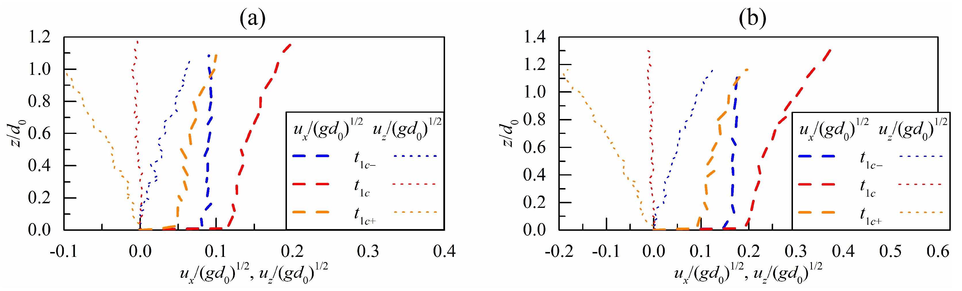
3.3.1. Incident Wave Characteristics

An impulse wave was subject to positive reflection at the slope, leading to higher wave amplitudes near the slope. According to the numerical simulation results, the wave parameters of an incident wave were approximated at x = 1.7 m to avoid wave reflection from the slope. The incident wave amplitude a_i is defined as the leading wave amplitude of the incident wave. Typical wave profiles for incident waves with different wave amplitudes are presented in Figure 7, where the abscissa is the time relative to the leading wave crest. Miller et al. [15] indicated that the leading wave of an impulse wave tends to be a solitary wave during its propagation. Therefore, the theoretical time series of a solitary wave with the same amplitude was also plotted in Figure 7 for comparison, which clearly indicates that the incident waves from the numerical simulation results differed considerably from the solitary wave profiles.

Figure 8 presents the distributions of the vertical velocity profiles beneath the leading wave for three typical moments—t_1c−, t_1c and t_1c+—where the subscript “1c” refers to the passage of the leading wave crest. t_1c− and t_1c+, defined at (d − d₀) = a_i/2, are the moments before and after leading wave crest passage, respectively. Each graph includes the dimensionless velocities u_x/(gd₀)^0.5 and u_z/(gd₀)^0.5 as functions of the relative vertical elevation z/d₀. The vertical velocity showed a linearly increasing trend with the vertical distance from the bed during the leading wave passage, consistent with Boussinesq’s findings [29]. The magnitude of the longitudinal velocities beneath the wavefront was approximately constant along the water column except near the bed, consistent with the first-order solitary wave equation [30]. In contrast, the longitudinal velocity beneath the leading wave crest and its subsequent wave surface exhibited an increasing trend when z increased. This trend deviated from the pattern derived from solitary wave theory.

3.3.2. Maximum Run-Up and Wave Force

The maximum run-up of an incident wave at slope a_r was defined as the maximum elevation of the leading wave crest at the slope. According to Hughes [31], the maximum run-up values of solitary waves on slopes can be predicted using the momentum flux parameter M*, which is defined as

$$\begin{array}{c}{M}^{*}=1/2\left({\left(a_i/d_0\right)}^2+2a_i/d_0\right)+N^2/\left(2O\right)\left(a_i/d_0+1\right)(\mathrm{t}\mathrm{a}\mathrm{n}\left(O/2\left(a_i/d_0+1\right)\right)+\\ 1/3{\left(\mathrm{t}\mathrm{a}\mathrm{n}\left(O/2\left(a_i/d_0+1\right)\right)\right)}^3)\end{array}$$

(5)

The expressions for N and O are as follows:

$$N=0.69\mathrm{t}\mathrm{a}\mathrm{n}\mathrm{h}\left(2.38a_i/d_0\right),$$

(6)

$$O=0.98{\left(\mathrm{t}\mathrm{a}\mathrm{n}\mathrm{h}\left(2.24a_i/d_0\right)\right)}^{0.44},$$

(7)

The relative maximum run-up a_r/d₀ for non-breaking and breaking incident waves is plotted against M* in Figure 9, where the solutions derived by Hughes [31] are shown for reference. Notably, incident waves with amplitudes larger than 0.47 tended to break up in their climbing processes along the slope, resulting in the discontinuity of the wave surface on the slope; hence, the corresponding run-up values were not available. As shown in Figure 9, the maximum run-up exhibits an increasing trend with the momentum flux parameter. In the range of 0.08 < M* < 0.62, the dataset for non-breaking incident waves consistently exhibited lower a_r/d₀ values when compared with the predictions by Hughes [31] for non-breaking solitary waves. The corresponding correlation coefficient R² is 0.86. However, due to limited data availability, the relationship between the breaking wave data and the predicted a_r/d₀ values for breaking solitary waves remained unclear.

In Figure 10, the non-breaking wave run-up data were further compared to the theoretical solution presented by Li and Raichlen [32] for non-breaking solitary wave run-up. The comparison revealed that when the dimensionless incident wave amplitude a_i/d₀ was less than 0.39, there was good agreement between the numerical and theoretical results, with an average relative deviation of 9.51% and R² = 0.99 for Li and Raichlen’s solution [32]. This finding aligns with the work of Miller et al. [15], who suggested that the maximum run-up of a non-breaking impulse wave at a slope can be estimated using solitary wave theory when its leading wave profile matches the theoretical profile. However, our results indicated similar findings even when the leading wave deviated from the corresponding solitary wave of the same amplitude in both wave profiles and velocity distributions. This suggests that this feature is independent of incident wave characteristics, which adds a new perspective to the existing understanding and highlights the robustness of the observed agreement across different wave conditions.

The dynamic wave force exerted on slope F_d is defined as the difference between the total force from the water and the initial static force. The dependence of the normalised maximum dynamic wave force F_dm/(ρgd₀²) on the relative incident wave amplitude a_i/d₀ is shown in Figure 11. As a_i/d₀ increased, the maximum dynamic wave force also increased. In the range of 0.07 ≤ a_i/d₀ ≤ 0.39, the maximum dynamic wave force of a non-breaking wave on the slope can be estimated from (R² = 0.956)

$$F_{dm}/\left(\rho g{d}_0^2\right)=2.136{\left(a_i/d_0\right)}^{1.129},$$

(8)

4. Conclusions

The safety of navigating ships and downstream structures in channel reservoirs, as well as human lives and properties on nearby slopes, are potentially threatened by landslide-generated impulse waves. In this study, numerical modelling of impulse waves generated by subaerial granular landslides was conducted using the open-source code of DualSPHysics. By coupling SPH and DEM methodologies, this complex fluid–solid coupling problem was addressed. An analysis of existing models for maximum wave amplitude prediction revealed that the predictive equation developed by Heller and Hager [16] showed better results when used with the slide centroid impact velocity for the slide Froude number calculation. Notably, the influence of slide shapes at slide impact on the accuracy of Heller and Hager’s model could be neglected. Furthermore, the maximum run-up heights of the impulse waves were found to be close to those predicted via solitary wave theory for non-breaking wave types. Additionally, it was discovered that the maximum dynamic force exerted by a non-breaking impulse wave depended on the incident wave amplitude in a power law. These findings contribute to a better understanding of impulse wave behaviour and provide valuable insights for assessing and managing landslide-generated impulse waves in channel reservoirs, with potential applications in early warning systems, emergency response planning, and mitigation measures.

References

1. Huang, B.L.; Yin, Y.P.; Wang, S.C.; Chen, X.T.; Liu, G.L.; Jiang, Z.B.; Liu, J.Z. A physical similarity model of an impulsive wave generated by Gongjiafang landslide in Three Gorges Reservoir, China. Landslides 2014, 11, 513–525. [Google Scholar] [CrossRef]
2. Huang, B.L.; Yin, Y.P.; Chen, X.T.; Liu, G.N.; Wang, S.C.; Jiang, Z.B. Experimental modeling of tsunamis generated by subaerial landslides: Two case studies of the Three Gorges Reservoir, China. Environ. Earth Sci. 2014, 71, 3813–3825. [Google Scholar]
3. Liu, Y.R.; Wang, X.M.; Wu, Z.S.; He, Z.; Yang, Q. Simulation of landslide-induced surges and analysis of impact on dam based on stability evaluation of reservoir bank slope. Landslides 2018, 15, 2031–2045. [Google Scholar] [CrossRef]
4. Wang, X.L.; Shi, C.Q.; Liu, Q.Q.; An, Y. Numerical study on near-field characteristics of landslide-generated impulse waves in channel reservoirs. J. Hydrol. 2021, 595, 126012. [Google Scholar] [CrossRef]
5. Ataie-Ashtiani, B.; Yavari-Ramshe, S. Numerical simulation of wave generated by landslide incidents in dam reservoirs. Landslides 2011, 8, 417–432. [Google Scholar] [CrossRef]
6. Tan, J.M.; Huang, B.L.; Zhao, Y.B. Pressure characteristics of landslide-generated impulse waves. J. Mt. Sci. 2019, 16, 1774–1787. [Google Scholar] [CrossRef]
7. Heller, V.; Hager, W.H. A universal parameter to predict subaerial landslide tsunamis? J. Mar. Sci. Eng. 2014, 2, 400–412. [Google Scholar] [CrossRef]
8. Huang, B.L.; Wang, S.C.; Zhao, Y.B. Impulse waves in reservoirs generated by landslides into shallow water. Coast Eng. 2017, 123, 52–61. [Google Scholar] [CrossRef]
9. Heller, V.; Spinneken, J. Improved landslide-tsunami prediction: Effects of block model parameters and slide model. J. Geophys. Res. 2013, 118, 1489–1507. [Google Scholar] [CrossRef]
10. Kamphuis, J.W.; Bowering, R.J. Impulse waves generated by landslides. Coast. Eng. 1972, 1972, 575–588. [Google Scholar]
11. Panizzo, A.; De Girolamo, P.; Petaccia, A. Forecasting impulse waves generated by subaerial landslides. J. Geophys. Res. 2005, 110, C12025. [Google Scholar] [CrossRef]
12. Walder, J.S.; Watts, P.; Sorensen, O.E.; Janssen, K. Tsunamis generated by subaerial mass flows. J. Geophys. Res. 2003, 108, 1–2. [Google Scholar] [CrossRef]
13. Wang, W.; Chen, G.Q.; Yin, K.L.; Wang, Y.; Zhou, S.H.; Liu, Y.L. Modeling of landslide generated impulsive waves considering complex topography in reservoir area. Environ. Earth Sci. 2016, 75, 372. [Google Scholar] [CrossRef]
14. Lee, C.H.; Huang, Z.H. Effects of grain size on subaerial granular landslides and resulting impulse waves: Experiment and multi-phase flow simulation. Landslides 2022, 19, 137–153. [Google Scholar] [CrossRef]
15. Miller, G.S.; Take, W.A.; Mulligan, R.P.; McDougall, S. Tsunamis generated by long and thin granular landslides in a large flume. J. Geophys. Res. 2017, 122, 653–668. [Google Scholar] [CrossRef]
16. Heller, V.; Hager, W.H. Impulse product parameter in landslide generated impulse waves. J. Waterw. Port Coast. Ocean Eng. 2010, 136, 145–155. [Google Scholar] [CrossRef]
17. Xu, W.J.; Yao, Z.G.; Luo, Y.T.; Dong, X.Y. Study on landslide-induced wave disasters using a 3D coupled SPH-DEM method. Bull. Eng. Geol. Environ. 2020, 79, 467–483. [Google Scholar] [CrossRef]
18. Fritz, H.M.; Hager, W.H.; Minor, H.E. Near field characteristics of landslide generated impulse waves. J. Waterw. Port Coast. Ocean Eng. 2004, 130, 287–302. [Google Scholar] [CrossRef]
19. Lindstrøm, E.K. Waves generated by subaerial slides with various porosities. Coast. Eng. 2016, 116, 170–179. [Google Scholar] [CrossRef]
20. Zweifel, A.; Hager, W.H.; Minor, H. Plane impulse waves in reservoirs. J. Waterw. Port Coast. Ocean Eng. 2006, 132, 358–368. [Google Scholar] [CrossRef]
21. Mohammed, F.; Fritz, H.M. Physical modeling of tsunamis generated by three-dimensional deformable granular landslides. J. Geophys. Res. 2012, 117, C11. [Google Scholar] [CrossRef]
22. Ataie-Ashtiani, B.; Nik-Khah, A. Impulsive waves caused by subaerial landslides. Environ. Fluid Mech. 2008, 8, 263–280. [Google Scholar] [CrossRef]
23. Heller, V.; Hager, W.H.; Minor, H.E. Scale effects in subaerial landslide generated impulse waves. Exp. Fluids 2008, 44, 691–703. [Google Scholar] [CrossRef]
24. Tan, H.; Chen, S.H. A hybrid DEM-SPH model for deformable landslide and its generated surge waves. Adv. Water Resour. 2017, 108, 256–276. [Google Scholar] [CrossRef]
25. Crespo, A.J.C.; Domínguez, J.M.; Rogers, B.D.; Gómez-Gesteira, M.; Longshaw, S.; Canelas, R.; Vacondio, R.; Barreiro, A.; García-Feal, O. DualSPHysics: Open-source parallel CFD solver based on Smoothed Particle Hydrodynamics (SPH). Comput. Phys. Commun. 2015, 187, 204–216. [Google Scholar] [CrossRef]
26. Canelas, R.; Ferreira, R.M.L.; Crespo, A.J.C.; Domínguez, J.M. A generalized SPH-DEM discretization for the modelling of complex multiphasic free surface flows. In Proceedings of the 8th International SPHERIC Workshop, Trondheim, Norway, 4–6 June 2013. [Google Scholar]
27. Canelas, R.B.; Crespo, A.J.C.; Dominguez, J.M.; Ferreira, R.M.L.; Gómez-Gesteira, M. SPH–DCDEM model for arbitrary geometries in free surface solid–fluid flows. Comput. Phys. Commun. 2016, 202, 131–140. [Google Scholar] [CrossRef]
28. Zhang, S.; Kuwabara, S.; Suzuki, T.; Kawano, Y.; Morita, K.; Fukuda, K. Simulation of solid–fluid mixture flow using moving particle methods. J. Comput. Phys. 2009, 228, 2552–2565. [Google Scholar] [CrossRef]
29. Boussinesq, J.V. Théorie de l’intumescence appelée onde solitaire ou de translation se propageant dans un canal rectangulaire. Comptes-Rendus L’acad. Sci. 1871, 72, 755–759. [Google Scholar]
30. Montes, J.S. Hydraulics of Open Channel Flow; ASCE Press: New York, NY, USA, 1998. [Google Scholar]
31. Hughes, S.A. Estimation of wave run-up on smooth, impermeable slopes using the wave momentum flux parameter. Coast. Eng. 2004, 51, 1085–1104. [Google Scholar] [CrossRef]
32. Li, Y.; Raichlen, F. Solitary wave runup on plane slopes. J. Waterw. Port Coast. Ocean Eng. 2001, 127, 33–44. [Google Scholar] [CrossRef]
Figure 1. Schematic layout of numerical model.
Jmse 12 01692 g001
Figure 2. Comparison of cylinder behaviours.
Jmse 12 01692 g002
Figure 3. Comparison of mass centre positions.
Jmse 12 01692 g003
Figure 4. Comparison of transient behaviours of water dam breakage.
Jmse 12 01692 g004
Figure 5. Typical shapes of slides at impact: (a) Type A, (b) Type B, and (c) Type C.
Jmse 12 01692 g005
Figure 6. Comparison of numerical results and am/d0 predictions (a) from Vsc0 and (b) from Vsc1; Fritz et al. 2004 [18]; Zweifel et al. 2006 [20]; Heller and Hager 2010 [16].
Jmse 12 01692 g006
Figure 7. Comparison between numerical and theoretical wave profiles: (a) R2, ai/d0 = 0.18 and (b) R10, ai/d0 = 0.34.
Jmse 12 01692 g007
Figure 8. Vertical velocity profiles beneath the leading wave: (a) R2, ai/d0 = 0.18 and (b) R10, ai/d0 = 0.34.
Jmse 12 01692 g008
Figure 9. Maximum run-up height as a function of dimensionless momentum flux.
Jmse 12 01692 g009
Figure 10. Comparison of numerical results and ar/d0 predictions from Li and Raichlen [32] for non-breaking waves.
Jmse 12 01692 g010
Figure 11. Maximum dynamic wave force vs. incident wave amplitude.
Jmse 12 01692 g011