Abstract
Over recent years, the emergence of the offshore wind sector has spurred much interest in subsea cables. The predominant failure modes of subsea cables are associated with extreme environmental conditions. Wave-forcing during severe storms is less expected and causes more damage. A generalized multiphysics cable model is constructed to predict the movement, damage, and lifetime of subsea cables subject to dynamic wave and current action due to abrasion and corrosion. The present cable lifespan prediction model extended the previous tide-only model by considering the contribution of hydrodynamic forces by waves and the effect of wave and current incident angle relative to the cable. The predicted cable sliding distance at each section of the cable is combined with the Archard abrasion wear model and the corrosion model to predict the loss of cable protective layers and the resulting expected lifespan of the cable. The model is the first of its kind that can predict the spatial variation of wave and current loading, cable movement, damage, remaining lifetime, and cable failure modes and location. In addition, spatial and temporal variations of magnitude and direction of wave, current, and tide can be incorporated into the model for realistic large-scale simulations of cable performance in field conditions. The model compares well with previous laboratory experiments and numerical models. The present model was applied for the first time to the European Marine Energy Centre (EMEC)’s wave test site located at Billia Croo off the west coast of mainland Orkney, Scotland, and validated by the cable lifespan data. The 1-year and 100-year return period wave height and period and the average wave and tide conditions are used to drive the present cable lifespan model. It was found that the cable movement is predominantly driven by waves, and the previous tide-only model would predict zero cable movement, indicating the importance of the incorporation of wave contribution into the cable model. Furthermore, besides wave height and period, the wave angle relative to cable was found to be a determining factor for the cable movement and lifespan. The present multiphysics cable model provides a new capability to predict 70% of failure modes currently not monitored in situ and to deploy, plan, and manage subsea cables with improved fidelity, reduced cost, and human risk.
Keywords:
subsea cable; underwater cable; lifespan; wave loading; submarine cables; abrasion; corrosion; offshore wind 1. Introduction
In 2021, it was reported that 97% of Scotland’s electric energy was from renewable sources [1,2]. Scotland is rich in natural renewable energy resources, such as wind, wave, and tide, with wind power being a significant driving force of Scotland’s renewable energy sector. Over 70% of Scotland’s renewable energy is generated by wind turbines [2]. The UK government’s decarbonization targets see the present 5 GW of offshore wind farms rising to between 20 GW and 40 GW in the next two decades at a cost of GBP 80 billion to GBP 160 billion.
The operation and maintenance (O&M) of wind farms have largely been ignored in research and development (R&D), with research to date focusing on wind turbines. These cables are often buried beneath the seabed, but sometimes they are left exposed on the seabed, in which case the cables may become damaged due to cyclic slide movement along the seabed. There is a lack of research on subsea cables, particularly regarding cable movement and lifetime.
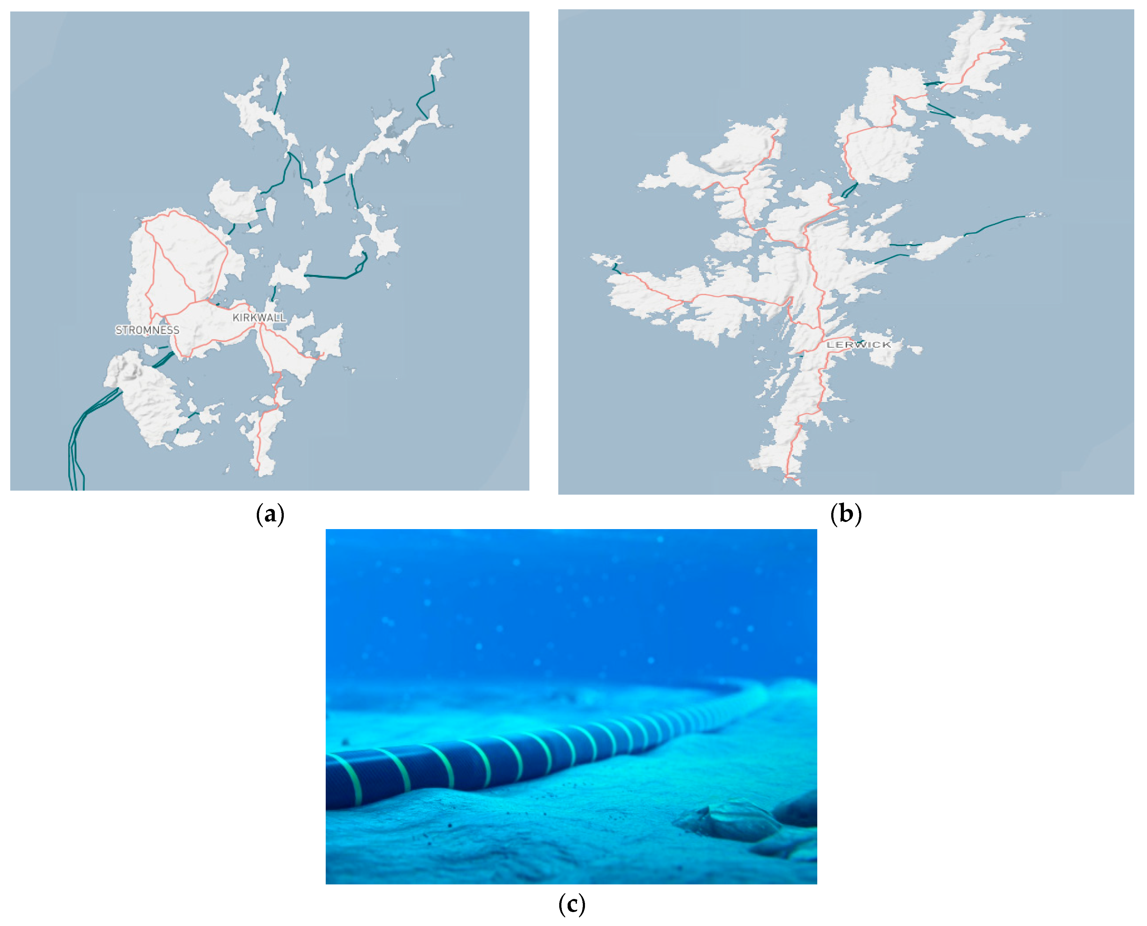
Power cables are one of the most critical assets within the offshore renewable energy infrastructure. These cables are vital to existing power distribution and transmission networks as well as the further development of offshore renewable energy installations. It is reported that global demand for these critical assets will also grow to an estimated total of 24,103 km over the forecast period, driven by the offshore wind cable demand that will grow at a 15% Compound Annual Growth Rate (CAGR), accounting for 45% of the forecast demand. The global submarine cable market is expected to grow four-fold from USD 6.31 billion in 2017 to USD 25.56 billion by 2026. According to GCube Insurance Services, subsea cable failures accounted for 77% of the financial losses in global offshore wind projects in 2015. Subsea cables are also found spanning short distances connecting remote island communities extensively in Scotland. Figure 1a demonstrates cable routes throughout the Orkney Islands, off the north coast of Scotland. The cable arriving from the south connects to the Scottish mainland. Figure 1b shows the cable routes throughout the Shetland Isles, even further north.

Figure 1.
(a) The unburied cables connecting Orkney Islands, off the north coast of Scotland, and (b) the cable routes throughout the Shetland Isles, further north of Orkney [3]. (c) Unburied subsea cable [4].
The cables are vitally important for these communities. The 21st-century advance into offshore renewable energy has led to highly engineered subsea cables, Figure 1c. However subsea cables are still at high risk of failure due to strong mechanical stresses from the action of the sea. In fact, over 40% of subsea cable failure is due to the effect of abrasion and corrosion [1]. Abrasion is caused by cable movement against the seabed; the distance the cable moves and the seabed roughness affect the level of abrasion. Natural slopes and rocks on the seabed may lead to the cable “free spanning”, where the cable spans over a gap. This exposes the cable to greater oscillation and fatigue. According to Scottish and Southern Energy (SSE)’s 15-year data set (http://sse.com/, accessed on 15 January 2022), the predominant failure modes of subsea cables are associated with extreme environmental conditions. A variety of extreme natural events, such as storms, tsunamis, earthquakes, landslides, and volcanic activities, may cause damage to subsea cables.
Cable failure causes unexpected power outages and damages the near-bed environment. For a 300 MW wind turbine, over 5 million pounds in revenue can be lost each month per cable fault [5]. Repairs may take months and cost a further million [1]. While extensive research has been dedicated to cable monitoring [6,7], less research has focused on cable failure predictions. However, 70% of the failure modes in subsea power cables are not detected by state-of-the-art monitoring techniques [1]. The lack of research and high failure rates indicate the need for a reliable mathematical model that can predict when a cable will fail. This would lower the risk of a cable failing unexpectedly and would allow time for cable repair or replacement.
Very few studies have been dedicated to predictions of damage and failures of subsea cables due to corrosion and abrasion [5]. A model was developed by Larsen-Basse et al. [8] to forecast the lifetime of a 40 m cable suspended between rocks in Alenuihaha Channel, Hawaii. The model focused on the localized abrasion wear on a section of cable without considering the full length of a cable or corrosion and scour. Wu [9] proposed a model to consider the effects of abrasion and corrosion on the lifetime of subsea cables. However, the model required the input of measured cable movement.
Dinmohammadi et al. [1] developed a software tool to estimate the lifetime of subsea cables by calculating the force of tidal currents acting perpendicularly on a cable and predicting the resulting movement of cables. The cable abrasion due to movement and cable corrosion was considered to predict when the cable would fail. This model, however, neglected the effect of wave loading and the angle between waves, currents, and cables. This was identified as a gap in the current literature. The present study provides the prediction for the movement and lifespan of a subsea cable due to wave, tide, and current actions to assist those responsible for the repair, monitoring, and design of subsea power cables.
The objective of this paper is to extend Dinmohammadi et al.’s [1] cable lifetime prediction model by incorporating the hydrodynamic forces by waves and the effect of wave and current incident angle relative to the cable for the first time to improve the prediction of movement and lifetime of subsea cables under wave and current forcing in dynamic environments.
2. Hydrodynamic Loading
A subsea cable is subject to a variety of mechanical stresses during its operational lifetime. An unburied cable is exposed to the combined stress of tidal current and wave force, comprising 3 components: horizontal drag, inertia force, and vertical lifting force. The inertia component comes from the water wave acceleration, whereas the drag force is due to the cable’s resistance to flow [10]. The lift force acts perpendicular to the water flow direction and is caused by the pressure zone formed on top of the cable [11]. The cable also experiences restoring forces such as submerged cable weight and seabed frictional resistance. Submerged weight is the weight of the cable in air minus the buoyancy force. Friction is a resisting force that exists when two surfaces move against each other, in this case, the cable and the seabed. The Morison Equation (2) expresses the horizontal hydrodynamic force as the sum of the drag and inertia force exerted by the flow on a horizontal circular cylinder of unit length perpendicular to the flow.
where and are the inertia and drag coefficients, respectively, is the density of seawater, is the cable diameter, the flow acceleration , and velocity are the sum of the components due to tidal current and wave motion and are functions of both time and space, i.e.,
The lift force and friction force are given by
where Ws is the submerged cable weight and µ is the bed friction coefficient.
are the horizontal wave velocity and acceleration perpendicular to the cylinder for a flat bottom according to linear wave theory [12], is the wave height, is the wave period, is the wavelength, is the water depth at which the cable is located, is the vertical distance from the mean free surface water level to the center of the cable, is the time, and is the wave radian frequency, is the wave number.
The hydrodynamic coefficients vary with Reynolds number and wave properties. Therefore, at each model run, suitable coefficients need to be selected. This can be done in a variety of ways. Ref. [3] identified a method to determine the hydrodynamic coefficients. When the acceleration is at its maximum during the wave period, the velocity is equal to zero. Therefore, the drag force equals zero, so the total force is equal to the inertial force, and therefore, the inertia coefficient is given by
Alternatively, when the velocity is at its maximum, the acceleration is at its minimum, so at that instant, the total force acting on the submerged object is equal to the drag force since the inertia force is equal to zero. Therefore, the drag coefficient is given by
To determine the lift coefficient, Equation (10) below [13], can be used. This paper assumes that the lift coefficient is a function of the maximum lift force in one wave period, i.e.,
Various researchers have conducted a wide range of tests to determine the inertia, drag, and lift coefficients. Sarpkaya [13] proposed that these coefficients vary with the Keulegan–Carpenter number (KC), Reynolds number, and other variables such as the Sarpkaya Beta value:
where is the amplitude of wave velocity, is the wave period, is the cable diameter, ν is the kinematic viscosity of the fluid. The KC value is a dimensionless number that describes the relative importance of drag forces over inertia forces in a flow. For a low KC value, inertia force will be the dominant force. Therefore, the drag force can be neglected [14]. As the KC increases, the drag becomes increasingly more dominant.
The bed frictional coefficient µ depends on the seabed type and the cable surface material. Generally, the coefficient increases with the roughness of the seabed. For example, a rocky seabed has a higher frictional coefficient than a clay-based bed. The measurements of frictional coefficients for a wire rope on the seabed are recorded in [15]. Table 1 lists some sample values of frictional coefficients, such as 0.25 for sand, 0.23 for mud with sand, and 0.18 for mud/clay for a wire rope on the seabed. Generally, it is more acceptable to use the “sliding friction coefficient” instead of the starting friction coefficient, which provides a more conservative result (friction data, n.d.).

Table 1.
Samples of bed frictional coefficients for wire rope over a seabed made of sand, mud with sand, and mud/clay [15].
3. Cable Modeling
In this section, the catenary cable model is constructed for current-only and current-plus-wave loading to predict cable movement. The predicted movement is combined with the abrasion and corrosion model to predict the cable lifespan.
3.1. Catenary Model
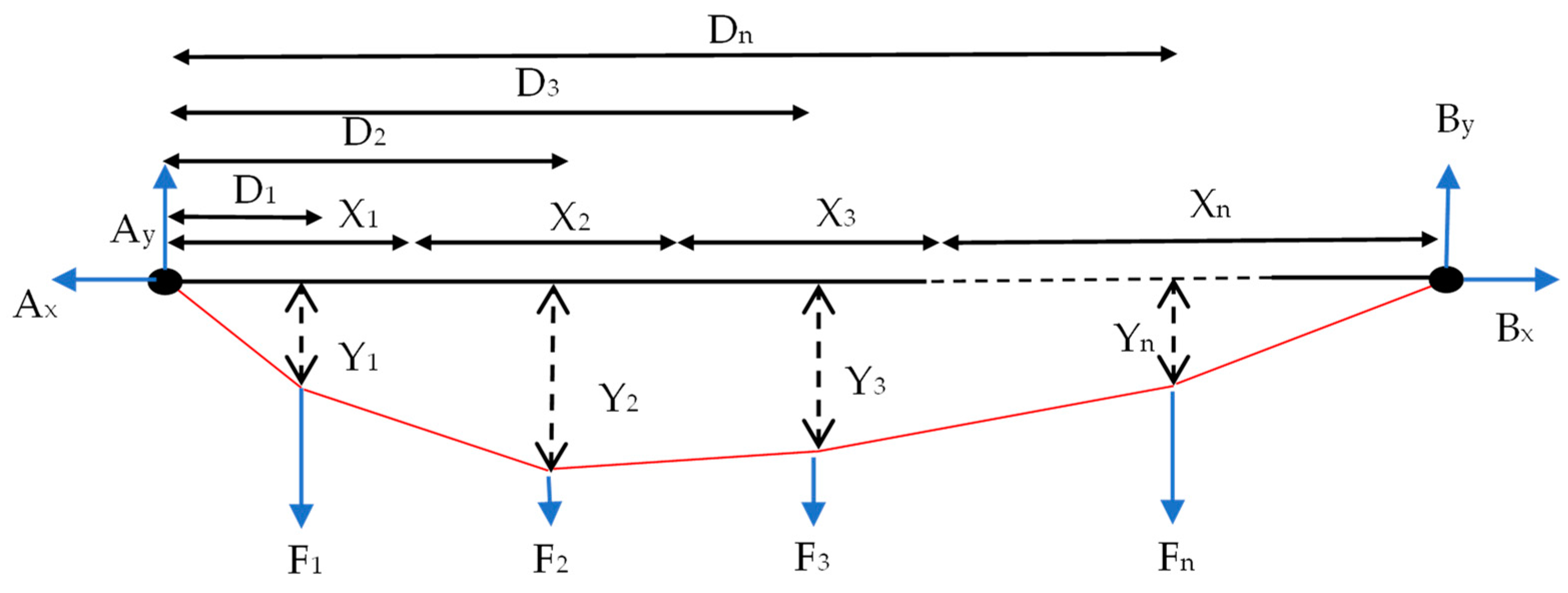
A catenary model is used here, similar to [1]. To increase accuracy, however, we assume the drag force to act at a concentrated point in the center of each zone. This is a common practice in engineering mechanics. Figure 2 shows the present model layout. The distance from the left-hand side of the cable to each zone center is denoted by , which runs from . As can be seen, the model is suitable for use in situations where the cable is fixed at each end. If a cable is buried, the drag force acting on it will be set to zero, and the cable will not move. The undisturbed bed friction velocity is given by [1].
where rbed = 2.5 × d50 is seabed roughness, and d50 is the representative diameter of the seabed sediment grain.
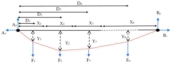
Figure 2.
Catenary model layout. The black horizontal line marks the cable’s original position, and the red line is the cable’s position once loading has commenced. The sliding distance of each zone to the equilibrium position is denoted by Yn. The length of each zone, denoted by Xn. F1, F2…Fn, is the resultant drag force acting on each cable segment at these zones. The cable is supported at both ends at points A and B. The reaction forces at the supports are denoted as Ax, Ay, Bx, and By.
3.2. Current-Only Loading
The total drag force for each zone along the cable is given by the Morrison equation,
where A is the cross-sectional area of the cable perpendicular to the tidal current, which is the product of cable diameter and zone length.
3.3. Current-Only Movement
The reaction forces perpendicular to the cable, at either end of the cable are given by the moment relative to the left end of the cable and the force balance in the y-direction.
Similar to Dinmohammadi’s model [1], it is assumed that the cable will move until it reaches a point of equilibrium as long as the net force is greater than zero. The point at which the cable reaches equilibrium is based on an assumed 1% slacking ratio, i.e., the cable can extend to a maximum length of 1.01 times the distance between points A and B.
When each loading point on a cable zone is at equilibrium, the moment due to the reaction in the y-direction will be equal to the moment due to the reaction in the x-direction, as shown in Equation (18) below. The horizontal reaction force, , is unknown. This can be found by summing the new cable zone lengths at equilibrium using Pythagoras’ Theorem and assuming that to be equal to the cable with a 1% slacking ratio [1], i.e., the cable is 1% longer than the straight distance between points A and B. The sliding distance is expected to change with the cable slacking ratio, which may vary in the real world. The sliding distance is expressed by Equation (19).
The corresponding equation in Dinmohammadi’s model [1] has a mistake: the term was written as . Pythagoras’ theorem states that the hypotenuse is equal to each of the other sides squared and summed together. Equation (19) rectifies this mistake. Once Equation (18) has been solved for the sliding distances to equilibrium for each cable zone can be found. A typical tidal flow pattern involves the tide going in and out twice a day, so multiplying the sliding distance to equilibrium by 8 would give the total sliding distance.
3.4. Current and Wave Loading
To consider the effect of combined wave and current loading, some of the governing equations in Section 2 need to be modified. First, the tidal current velocity is added to the wave motion velocity to obtain the flow velocity. Second, as shown in Equations (4) and (5), it is assumed that the wave motion is acting directly perpendicular to the cable. For the wave and current approach, the cable at an oblique angle of α and , the flow velocity and acceleration becomes
In the case that hydrodynamic forces are perpendicular to cable, and .
Unlike current-only loading, the forces acting upon the cable vary with time in both magnitude and direction in the presence of a wave, so for each cable zone, the force on the cable must be calculated at every chosen time interval of the wave period. The net force acting on the cable is derived by subtracting the frictional resistance from wave and current loading predicted by the Morison equation. This time, however, the horizontal wave force can be negative at some time-steps during the wave period. Since the cable is assumed to be on the ground, the lift force cannot be negative (downward) [16].
The time-step was chosen at 0.5 s. To verify the model convergence at this time-step, time-steps of 2 s, 1 s, 0.5 s, and 0.25 s were compared. For each time-step, drag force was calculated for a cable of 13 zones. As shown in Figure 3, the model results converge around a time-step of 0.5/0.25 s. Hence, a time-step of 0.5 s was presumed to be suitable for normal use of the model. If necessary, the time-step can be easily refined in the model.
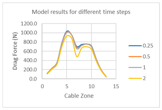
Figure 3.
Model sensitivity to time-step. The drag forces predicted by Equation (1) along the cable (x-axis) for time-steps of 0.25, 0.5, 1, and 2 s.
3.5. Cable Movement under Current and Wave Loading
Unlike current loading, wave loading is a time- and space-dependent variable in magnitude and direction. Therefore, in this scenario, the maximum sliding distance until equilibrium was calculated for each time-step during the wave period. This was deemed acceptable since the net forward force of the wave will also carry the cable forward until it reaches an equilibrium position. This equilibrium position is assumed as the maximum equilibrium distance out of all the time-step values. Once the cable reaches this position, it cannot move any further forward due to the 1% slacking ratio of the cable.
Up to this point, this process has been similar to the current-only sliding distance calculation. However, the major difference in sliding distance in the presence of a wave is the potential backward motion of the cable due to backward flow motion.
A backward force is exerted on the cable every wave cycle if it can overcome the frictional resistance. The model discussed here accounts for this backward movement once it reaches its equilibrium position. The equilibrium position is the point where the cable cannot extend any further forward but can move backward due to wave loading. Backward moving will occur as the cable moves out to this equilibrium position, but this is assumed to be negligible.
To calculate backward movement, the equations of motion were used.
For every calculated backward moving force at Xi, the cable acceleration d2Yi(t)/d2t was derived by dividing the force per unit length by the mass of the cable per unit length at Xi. From the acceleration, the cable velocity and then the relative cable velocity to the water was calculated. This allowed the cable sliding distance to be evaluated for every time-step. The sum of these distances was multiplied by 2 to account for the cable movement back to its original equilibrium position.
A different approach is required when the drag force acting on the cable has equal forward and backward movement, i.e., when wave only is considered and tidal velocity is equal to zero. Here, the cable may not reach the position where it cannot extend further, i.e., the equilibrium position, before it moves in the opposite direction. The cable will remain central and will move forward and backward during each wave period as long as the wave force can overcome the friction.
3.6. Abrasion and Corrosion
Both single- and double-armored cables are considered in the present model. Figure 4 shows the cross-section, materials, and layers for a subsea power cable. Failure is assumed when these armored layers are fully worn away by the combined effect of abrasion and corrosion. Similar to [1], corrosion is neglected for the outer bituminous layer compared to abrasion. For carbon steel, the corrosion penetration rate is assumed to be 4 mm/year [16], and for stainless steel, 0.07 mm/year [17].
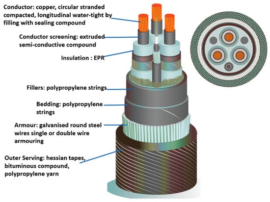
Figure 4.
Cross-section and materials and layers of a subsea cable [1].
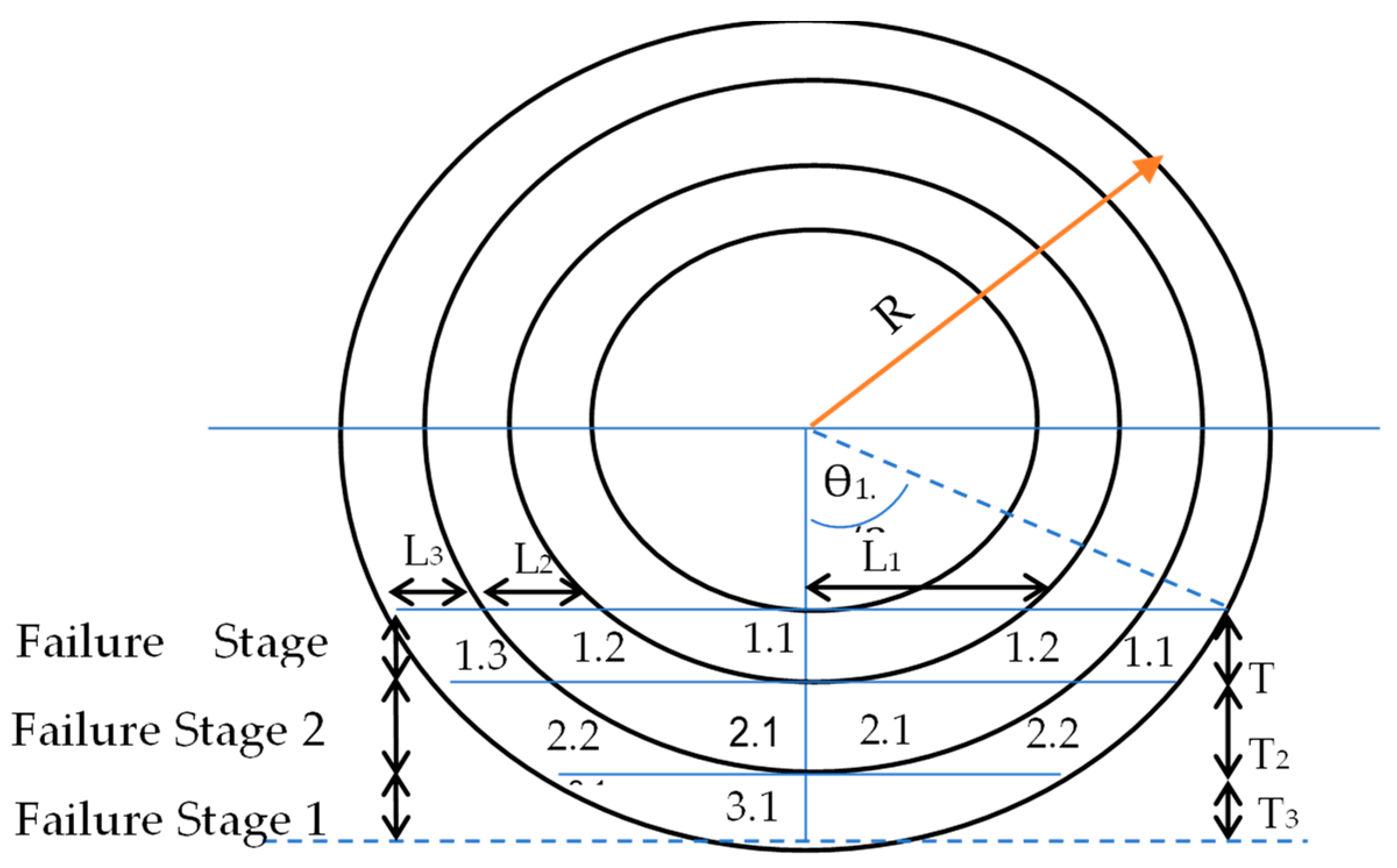
The armor is affected by corrosion and abrasion. Figure 5 below demonstrates the 3 stages of abrasion. Once layer 3 has been worn down, abrasion will start on layer 2 and so on. If the cable is single-armored, corrosion will only occur in zone 1.1. If the cable is double-armored, then corrosion occurs in zones 1.1, 1.2, and 2.1.
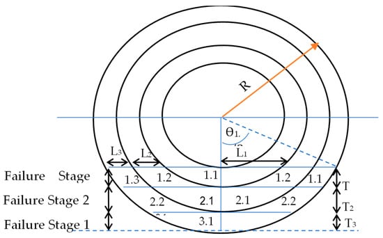
Figure 5.
Cable failure cross-section. The example cable is a double-armored cable with two inner layers (1 and 2) made of steel/steel wire. R is the radius of the cable, ϴ is the angle between each cable layer section and the vertical line, and T is the layer thickness. All these variables are required to calculate the volume of each section.
Every zone volume must be calculated to estimate when the cable will fail. Following [1], the widely used Archard abrasion wear model [18] has been adopted. The corrosion wear model by Qin and Cui (2003) [19] is used to derive the abrasion and corrosion volume.
where is the abrasion wear coefficient, is the sliding distance, and is the cable hardness. is the submerged weight of the cable, is the corrosion penetration rate, and can either be assumed as 0.33 or 1 [20], , is the area of the cable exposed to seawater, is the length of time after the cable has been laid, and is the lifetime of the corrosion protection coating. While the abrasion rate is constant throughout the life of the cable, the corrosion rate is a function of time. Similar to Qin and Cui (2003) [19], it is assumed that corrosion will not start until the corrosive protection layer on the metal has been worn down. This can be due to corrosion itself; a 5-year lifetime for the coating is regarded as being undesirable, and a 10-year lifetime as being desirable [20]. However, it should be noted that if the cable is subject to high sliding distances, the corrosive layer may be worn down before the 5- or 10-year lifetime is reached.
The outward protective materials include bitumen or polypropylene and metal armoring such as steel wire. Due to a lack of data, Dinmohammadi et al., 2019 [1], explain how testing was carried out to provide suitable wear coefficients for the above materials in consultation with the British Approvals Service for Cables (BASEC). Table 2 shows the results. The abrasive wheel types represent the coarseness of the wheel. The lower the number, the coarser the material. H10 represents a coarse material, H18 a medium coarseness and H38 a very fine material. A wheel type that is most like the seabed where the cable is to be laid should be used in this model.
Table 2.
Wear coefficients of 3 types of materials [1].
Corrosion penetration data for steel and other metals are available; however, there is a lack of information regarding corrosion penetration for bitumen or polypropylene [1]. We assume that the corrosion wear is negligible since the abrasion wear is dominant for this part of the cable.
Once the abrasion wear rate is calculated, the expected lifetime of the cable, EL, is obtained using the formula:
where is the total volume that can be lost due to corrosion and abrasion in each layer. In this formula, it is assumed that once 100% of the cable’s protective layers are worn down. The total volume of the protective layer is equal to the volume worn down by abrasion and corrosion.
The model allows an input of a percentage of the total wear volume of the steel layer. If this value is reached before the natural coating lifetime is reached, corrosion will automatically start.
The total wear over time will be combined for each cable section. Once this value is equal to the section volume, that section will be assumed to be disintegrated. The volume of each layer section must be calculated.
4. Model Verification
The predicted cable movement is verified against Dinmohammadi’s model [1] for tidal current-only conditions. Then, the predicted wave loading and the abrasion and corrosion model are validated by the experiments by Neelamani and Al-Banaa (2012) [21] and Qin and Cui (2003) [19], respectively.
4.1. Cable Sliding Distance
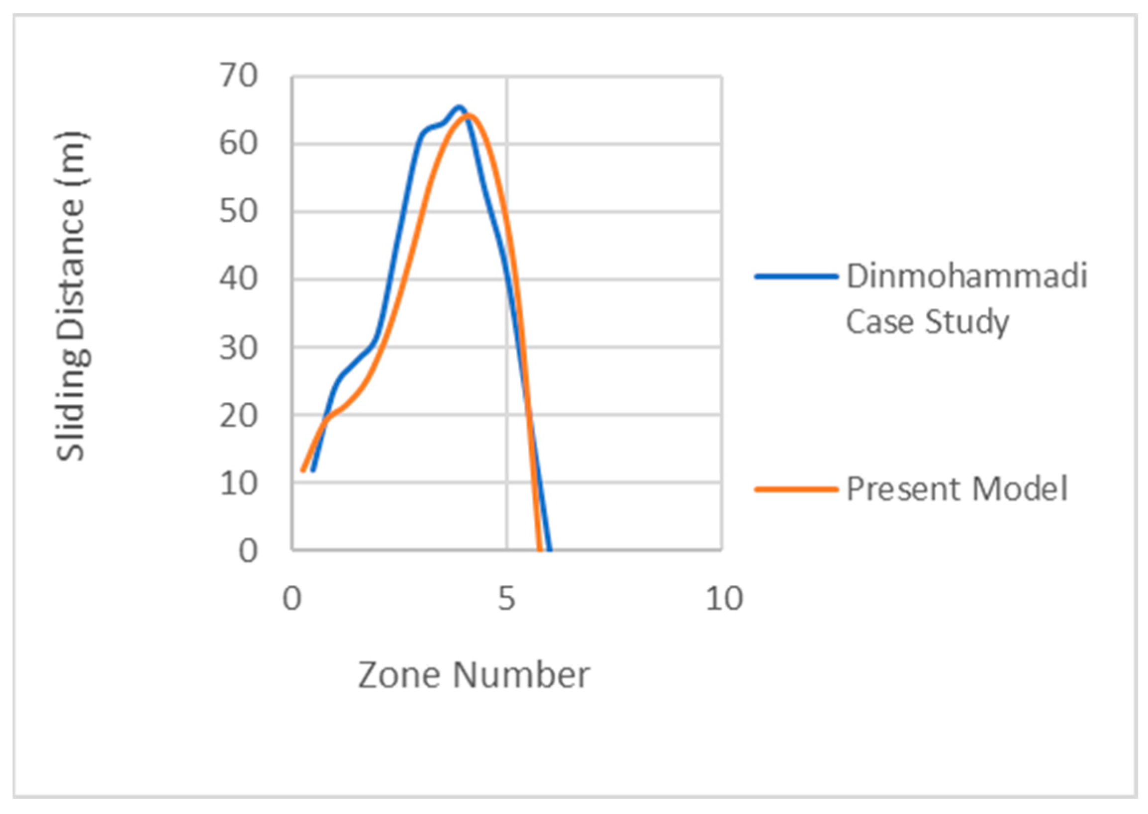
Following Dinmohammadi et al. [1], a case study is carried out to demonstrate how the model functions. It employs 13 cable zones on a 2.1 km cable between two islands with varying tidal velocities and cable lengths. The first seven zones from that case study were used to verify the present model. The present model ran 14 zones to increase accuracy with the data used in Dinmohammadi’s paper. The sliding distance until equilibrium from the present model and Dinmohammadi et al. [1] compare well in Figure 6.
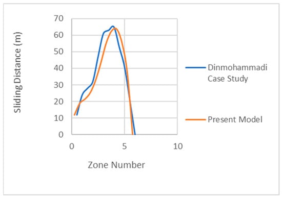
Figure 6.
Cable sliding distance predicted by the present model (red) and Dinmohammadi’s [1] model (blue). The cable sliding distance until equilibrium is shown on the y-axis. The x-axis marks each cable zone.
The phase difference is because the cable sliding distance is calculated at the end and center of each zone in Dinmohammadi’s [1] model and the present model, respectively. As can be seen, this decision does have some disadvantages, as the buried zone only seems to be stationary at a single point in the cable. Dinmohammadi’s model captures this better. However, for the calculation of life expectancy, the most important variable is the maximum sliding distance since it is assumed that this zone will fail first. As can be seen from the comparison, the peak sliding distance predicted by the present model is in good agreement with Dinmohammadi’s [1] model results. However, if a cable is to experience a scenario where multiple zones become self-buried due to scouring, results may vary greater.
4.2. Wave Loading
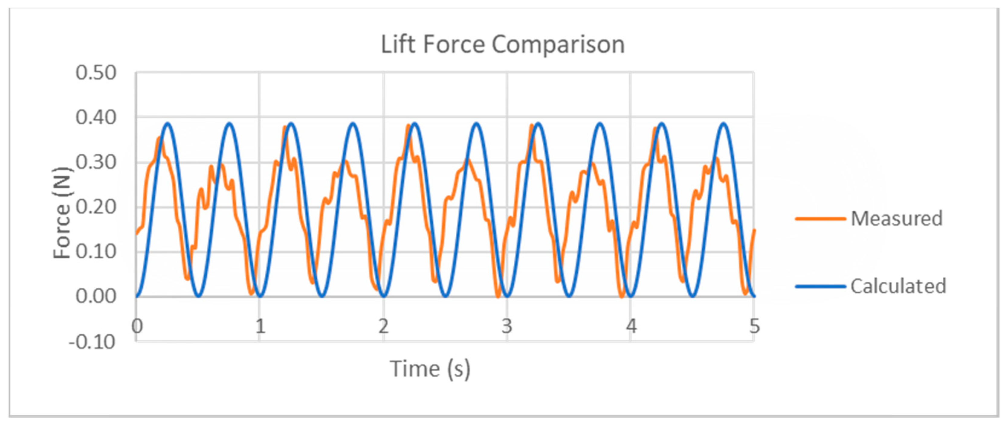
Figure 7 and Figure 8 below show the validation of calculated horizontal in-line forces and vertical lift forces against the experiment of a submarine cable under a wave [19]. The experiment was conducted for a cable with a diameter of 20 cm and a length of 0.597 m, lying on a synthetic seabed at a depth of 45 cm under a regular wave with a height of 5 cm and a period of 1 s.
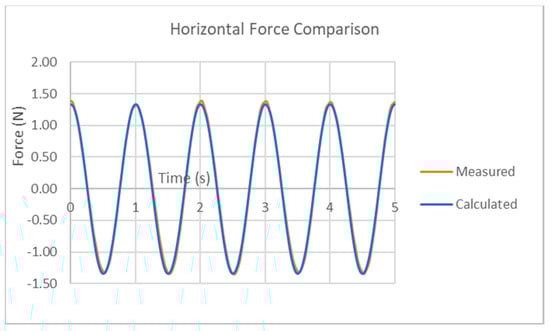
Figure 7.
Comparisons of the predicted horizontal force (blue line) by the present model and the experiment by Neelamani and Al-Banaa (2012) (orange line) [21].

Figure 8.
Comparisons of the predicted Lift force (blue line) by the present model and the experimentation (orange line) [21].
From the experimental data in Neelamani and Al-Banaa (2012) [21], the drag, inertia, and lift coefficients could be derived as , and .
As can be seen from Figure 7, the horizontal force per unit length results from the present model are almost identical to the experimental measurements [19]. There is more variation in the lift force comparison in Figure 8, with a time average error of around 5%. The model still captures the peak loads reasonably well, but this may result in slightly lower values of frictional resistance.
4.3. Cable Lifetime
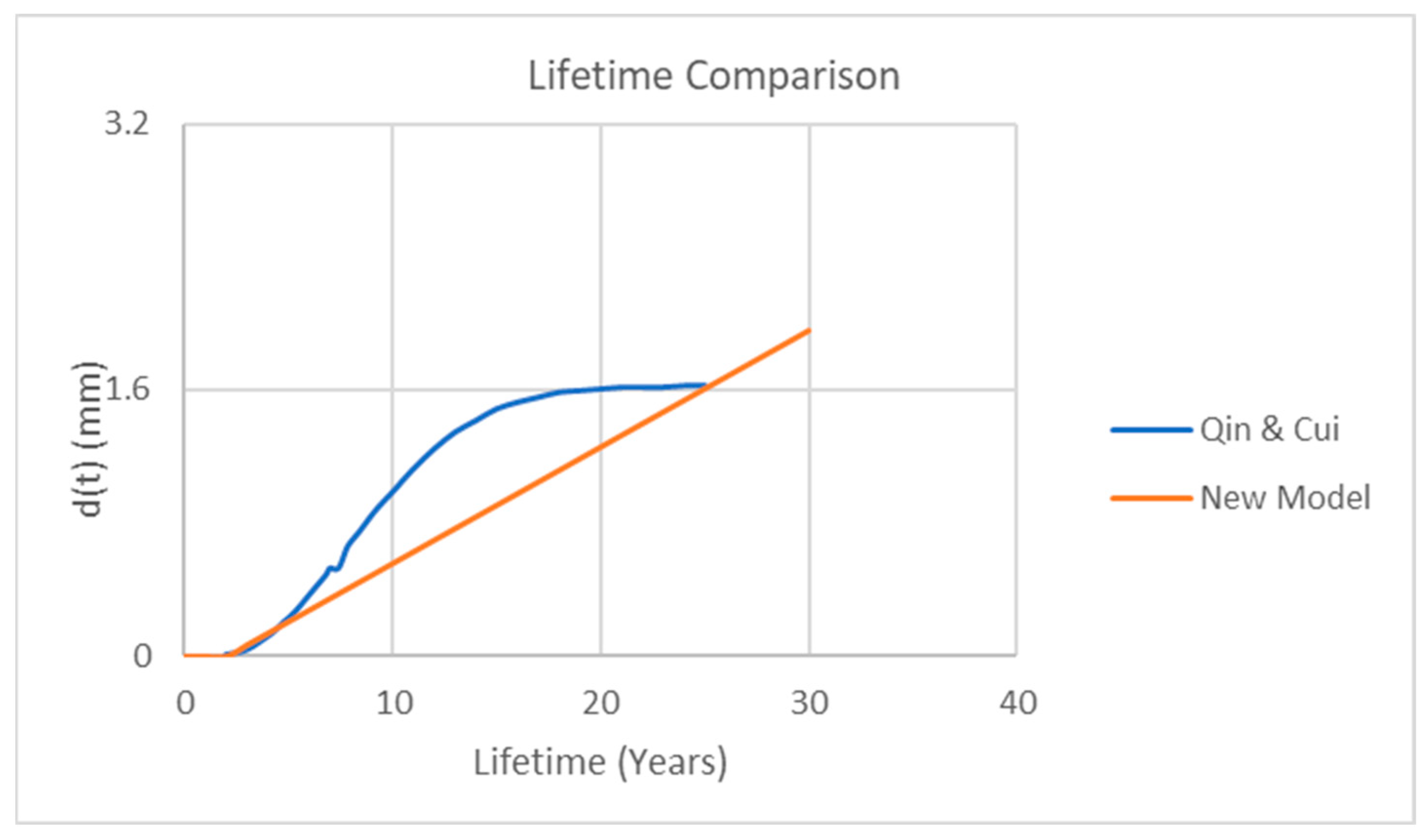
A corrosion testing experiment demonstrates the life expectancy of a flat steel plate of 1.6 mm depth [20]. It was found that the plate has a lifetime of 25 years. When verifying these results using the present model, a slight change had to be made to the code. The present model calculates the total volume lost due to corrosion and compares it to the total zone volume, whereas the corrosion test experiment compares the total thickness lost due to corrosion and compares it to the total thickness. Therefore, the model had to be adapted to the following:
where dplate is plate depth, t is time, and Tcoating is the lifetime of corrosion coating. The corrosion penetration rate (, was assumed as 0.07 mm/year, and a value of 1 was chosen for . The result, Figure 9, estimates a lifetime of 25 years since the wear rate reaches 1.6 mm around this time. There is a clear verification of life expectancy. While this verification does not account for the exact procedure undertaken in the model, it is assumed to be similar enough to justify this verification.
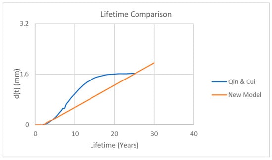
Figure 9.
Corrosion wear verification. Using Equation (28), the wear rate will ultimately result in 1.6 mm of corrosion wear by 25 years.
5. Case Study of EMEC Field Site
The present model is applied for the first time to the European Marine Energy Centre (EMEC)’s wave test site located at Billia Croo off the west coast of mainland Orkney, Scotland, and validated by the cable lifespan data. The 1-year and 100-year return period wave height and period and the average wave and tide conditions are used to drive the model.
5.1. EMEC Field Site
Established in 2003, the European Marine Energy Centre (EMEC) provides purpose-built open-sea testing facilities for wave and tidal energy.
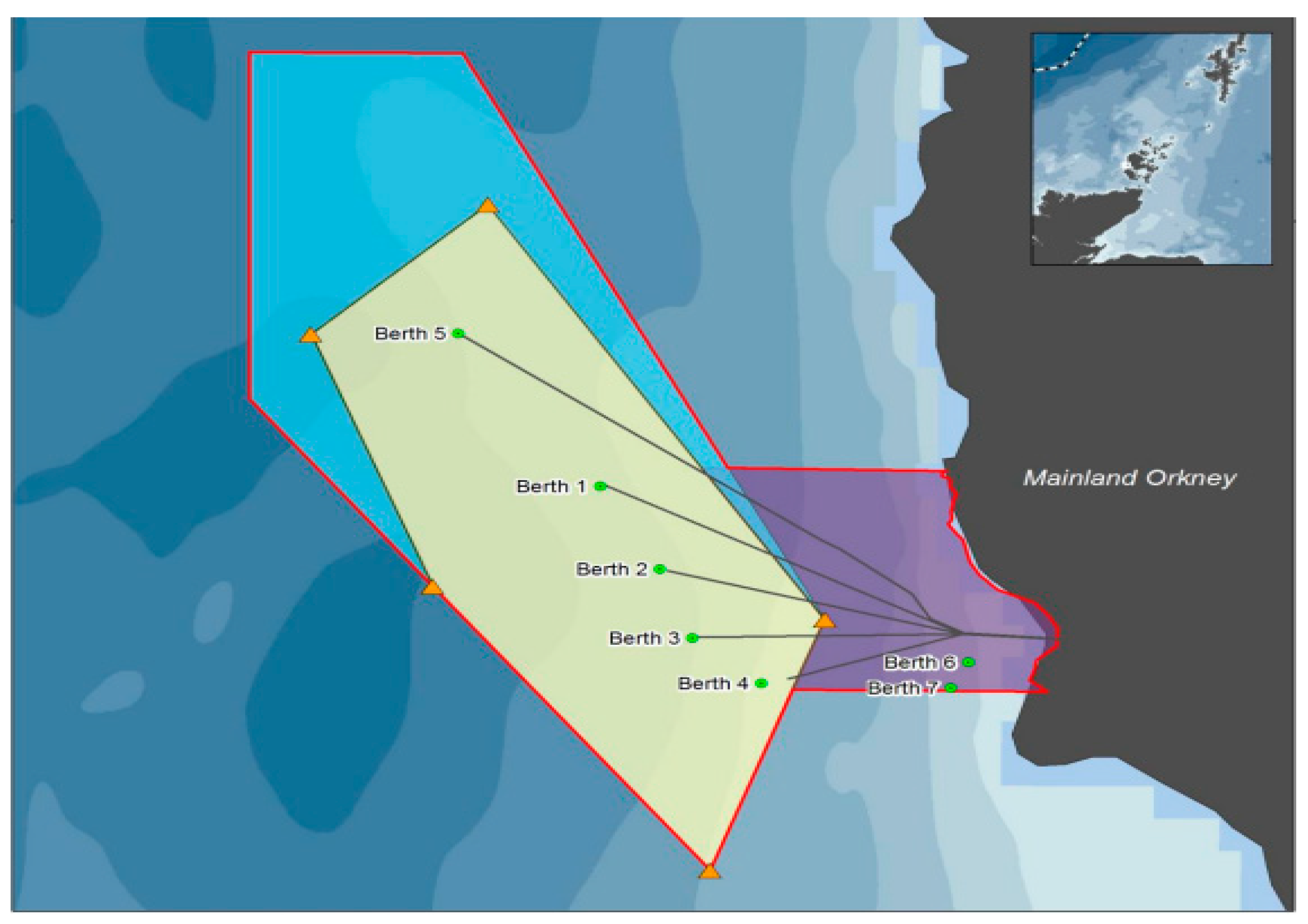
EMEC’s wave test site is grid-connected and located at Billia Croo (Figure 10), off the west coast of mainland Orkney. The site is subject to large waves from the west and northwest, originating in the North Atlantic Ocean. The site has five test berths in the offshore area and two near-shore test berths linked by armored cables to a substation onshore.
As listed in Table 3, wave data for 1-year and 100-year return periods, which is expected to occur once in 1 year and 100 years on average from EMEC’s Directional Waverider buoys is provided by Draycott, Davey, and Ingram (2017) [22], and the average wave conditions can be found at the EMEC website [23]. To compare, storm wave properties with a 1-year return period and a 100-year return period will be input into the present model, as well as the average properties from the test site.
Table 3.
Wave parameters with a 1-year return period and a 100-year return period used in the case study.

Figure 10.
Wave testing site at Billia Croo [23] at the EMEC. The cable running to berth 3 (second from the bottom) was chosen for this case study.
Figure 10.
Wave testing site at Billia Croo [23] at the EMEC. The cable running to berth 3 (second from the bottom) was chosen for this case study.
A tidal velocity of 1 m/s was used for both scenarios [23]. The seabed sand diameter was assumed to be 62.5 m.
5.2. Cable Properties
The cable running from the mainland to berth 3 will be considered. The cable contains 2 layers of galvanized steel wire. Data from EMEC’s cable lifecycle study [24] gave the following cable information, which was input into the model:
- 50 mm2 cross-sectional area
- 0.008 m
- Length of 2 km
- At a depth of approximately 60 m
- Cable weight: 30 N/m
Other cable properties were not available and had to be estimated as follows:
- Drag coefficient: 1.2
- Lift coefficient: 1.2
- Inertia coefficient: 3.1
- Friction coefficient: 0.2
- Steel wear coefficient: 0.02773
- Propylene wear coefficient: 0.000883
- Steel hardness (N/m2): 1.7 × 10⁹
- Propylene hardness (N/m2): 5.0 × 10⁸
- Thickness of each layer constant at 0.001 m
- Corrosion Penetration Rate for steel is 1.92 × 10⁻⁷ m/day
5.3. Model Results
Wave incident angles of 0, 15, 30, 45, and 75 degrees were used to demonstrate the impact of wave approach angle on cable lifetime. The lifetime properties are summarized below in Table 4, with all results being in years:
Table 4.
Predicated lifetime (year) for wave incident angles of 0, 15, 30, 45, and 75 degrees. N/A indicates the wave and tide current loading less than the bed friction with no cable movement.
As expected, when the average wave properties were used by the model, the longest lifetime was predicted. This value should be used as an indication of the total expected lifetime for the cable. The storm weather results are also as expected, with the model predicting longer lifetimes for these cases. An incident angle of 0 means the wave is approaching perpendicularly; hence why lower lifetimes are calculated. For some of the large incident-wave angles and wave height and period, despite the same tidal current loading for all wave incident angles, the model predicts that the hydrodynamic forces will be unable to overcome the frictional forces acting on the cable from the seabed. The model is unable to predict a lifetime in this case. This limitation is discussed in the conclusion. This result indicated that the cable movement at this site is dominated by wave action, and the previous tide-only model by Dinmohammadi et al. [1] would predict zero cable movement. This result indicates the importance of the incorporation of wave contribution in the cable model.
The predicted cable movement every 24 h is shown below in Table 5. All results are in meters:
Table 5.
Predicated cable movement (m) in 24 h for wave incident angles of 0, 15, 30, 45, and 75 degrees.
The predicted total horizontal loading (horizontal loading minus friction) acting on the cable with 1-year return period wave data is listed in Table 6.
Table 6.
Time history of predicated total horizontal loading in N/m for 1-year return period wave conditions.
The predicted horizontal loading (horizontal loading minus friction) acting on the cable with 100-year return period wave data is listed in Table 7.
Table 7.
Time history of predicated total horizontal loading in N/m for 100-year return period wave conditions.
The predicted horizontal loading (horizontal loading minus friction) acting on the cable with average wave data is listed in Table 8.
Table 8.
Time history of predicated total horizontal loading in N/m for average wave conditions.
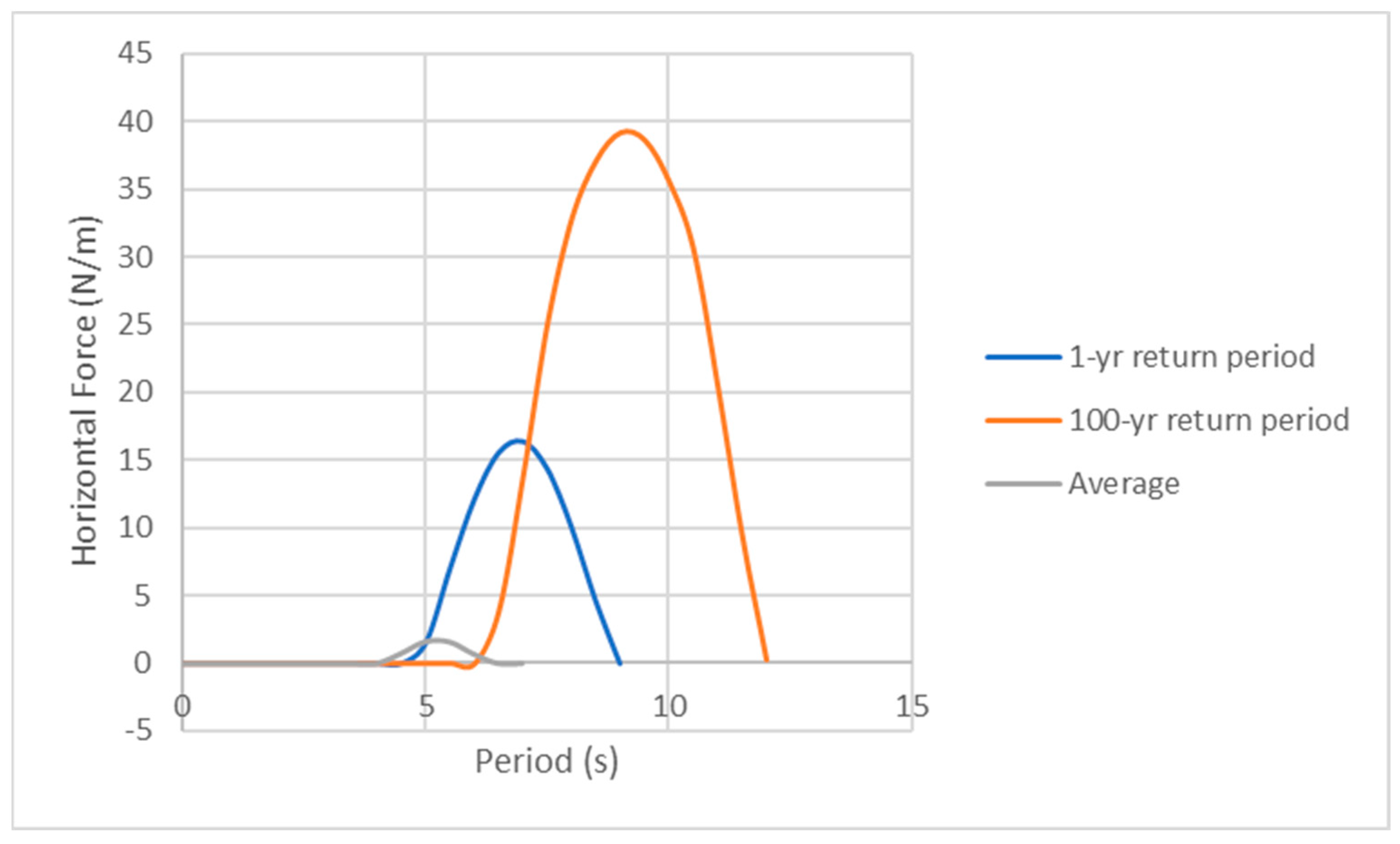
Figure 11 below demonstrates the drag forces acting on the cable for 1-year, 100-year, and average wave conditions and zero incident-wave angle.

Figure 11.
Horizontal loading for 1-year, 100-year, and average wave conditions and zero incident-wave angle.
5.4. Case Study Discussion
At the test site, the cable is approximately 75° to the approaching wave and tidal forces. Although this is not constant, it is assumed to be so in this case study. While no result for this angle was found for the average wave properties, the model clearly predicted a lifetime of at least 7.1 years for the cable. The variation of lifetime against wave approach angle is reasonably small, as seen from the 1- and 100-year results. Hence, it could be estimated that the cable would fail before 10 years, with at least one cable section failing.
The data from EMEC [22], however, shows a different result, and it highlights one major limitation of the model. The cable was placed in 2003, and it was lifted onshore several times throughout the following years for tests and some minor repairs. A remotely operated vehicle (ROV) was used to monitor the cable in 2013 and showed that while some of the outer propylene had worn away and exposed the metal, the cable had not failed. According to the EMEC [23], this was “remarkable”.
One reason for the model results differing is the nature of the seabed where the cables are laid. The cables are mainly in free span at this site [23], meaning that the cable was not experiencing abrasion to the level that the model assumed it was. Currently, the model does not account for this situation, where certain areas experience abrasion, and others do not. This is something that could be worked upon later.
The model predicts failure between 7 and 10 years, and the EMEC data shows a lifetime of more than 10 years, although this was unexpectedly high. However, the EMEC cable was repaired several times during its service. Taking account of this and the regular cable spans, the EMEC data do not contradict the model.
5.5. Model Limitations
The catenary model used in this work does not account for as many factors as sophisticated cable models and flexible slender structure models [24,25], e.g., cable stiffness, although this can be accounted for to some extent in the case of scouring with the selection of reduction factors. The stiffness of the cable would impact the relationship between the different cable zones. A higher stiffness would mean less bending between zones, which, in turn, could lead to a lower sliding distance or a higher sliding distance, depending on the stiffness. Similarly, the model does not consider elasticity, i.e., the ability of an object to return to its original position after unloading, which was incorporated in [25]. This could affect cable sliding distance.
Individual zone deformation is also ignored in this model. The cable zones act as one regarding their movement. With larger cable lengths, the model can become less accurate.
Boundary layers exist whether current flow only is assumed or when wave force is included [26]. This model does not account for the boundary layer. This can cause a negligible impact if the cable has a large diameter and extends well beyond this zone.
The Morison equation has a number of limitations. First, it assumes that water acceleration is uniform when it arrives at the cable [27]. For small structures, however, this assumption is sufficient. The general rule is that if the cylinder diameter is smaller than the wavelength, the assumption is acceptable. Therefore, this will practically always be valid for subsea cables [28,29,30]. The Morison equation may fail to accurately describe the force–time history of the wave loading. However, the coefficients, if selected well enough, allow for an accurate depiction of the extreme force values, i.e., the highest and lowest numbers.
The choice to use the equations of motion to calculate sliding motion has the potential to be one of the largest sources of error within the model. These equations function in a scenario of constant velocity and, therefore, constant movement. This model calculates the cable velocity and movement for every 0.5 s time-step. If, theoretically, the time-step was small enough, this method would be more accurate. However, due to time constraints, this method was employed for this model. In due course, this must be improved for full functionality. If the backward motion is negligible due to friction, then the model is more accurate. The designer should note that if this is not the case and backward cable motion does exist, then the sliding distance has the potential to be too high an estimate. Alternatively, in the event that forward and backward forces are equal, the sliding distance will also be a very high and inaccurate estimate.
In the scenario where either the forward or backward force is larger than the other, the model does not account for cable oscillation as the cable moves toward the equilibrium point. For example, if the resultant wave force moves the cable forward and backward, movement also does occur. This movement will not just occur on the equilibrium line. Backward movement will occur for each wave period while the cable moves in the wave’s resultant direction. This model does not account for this and assumes the majority of backward sliding will occur at the maximum equilibrium position. This assumption is generally valid but could lead to inaccuracy in certain circumstances, i.e., if the net forward wave force is only slightly larger than the net backward force.
While this model is only applicable for unburied cables, the model does account for cable scouring. In the unlikely event that cable scouring occurs for all the cable zones, this model is not suitable for use. This is because movement for a scour zone is assumed to be zero, and, therefore, abrasion is assumed to be zero. The outer layer wear in this model only accounts for abrasion, and, therefore, it will not be able to produce an acceptable life prediction for this scenario.
A cable being caught by a trawler or otherwise being negatively impacted by a human-made disturbance will significantly shorten a cable’s lifetime. This model does not account for this. Extreme weather cases will cause short-term but potentially large increases in sliding distance. Underwater obstacles can also block or prevent cable movement. Perhaps one of the biggest uncertainties of the model results comes from varying tidal currents and wave properties. Each time the model is run, these variables are assumed to be constant for the lifetime.
6. Conclusions
In this paper, the previous cable lifetime prediction model was extended by incorporating hydrodynamic forces by waves and the effect of wave and current incident angle relative to cable. The present model was verified by experimental data and previous models. This generalized cable prediction model can be employed in a wider variety of wave and current conditions, locations, and scenarios compared to the previous model.
The present model was applied for the first time to the European Marine Energy Centre (EMEC) wave test site located at Billia Croo off the west coast of mainland Orkney, Scotland, and validated with cable data. The wave data for 1-year and 100-year return periods and the average wave and tide conditions were used to drive the present model to simulate the cable response to extreme and average environmental conditions. It was found that waves have a dominant effect on cable movements compared to tidal currents at this site. Besides wave height and period, wave angle relative to cable was found to be a determining factor of cable movement and lifespan.
The model discussed here has not been done before and is, therefore, an improvement in the field of subsea cable design and research. No other model allows assessments of cable movement and lifetime under both wave and current loading. This model is unique in that regard and robust for a large-scale field study of cable lifespan. It provides new and improved capabilities for cable monitoring, design, maintenance, and route selection.
As with other models, the present model has its limitations, as discussed in Section 5.5. The model is dependent on cable location, input properties, and the nature of the final results (see Section 4.3 on cable movement). It should be noted that a nominal value of cable property has been used to demonstrate the performance of the present model when a true value is not available. It is worth carrying out systematic parametrical studies of the effect of various cable properties on cable movement and lifespan in the future.
The present model can be combined with a high-resolution wave model and substrate map to improve its prediction capability at a field site. The slacking ratio can be adapted for a cable route at a selected site. Burial and unburial of the cable due to sediment transport and morphology change and scour under dynamic tide, wave, and seabed conditions can be incorporated into the model [31,32,33].
Besides the hydrodynamic force discussed above, fish trawling and anchoring are two of the major causes of cable failure. The mechanical, electrical, and thermal behavior of the cable may also affect cable function and lifetime [34,35]. Multiphysics and structural health monitoring (SHM) through embedded sensors and sonar technology such as fiber-optic sensors [36] and wideband low-frequency sonar [37,38] approaches have been proposed to monitor the integrity of cables. Monitoring techniques can be targeted at the potential weak spots of a cable predicted by the present model.
Author Contributions
Conceptualization, Q.Z. and D.F.; Methodology, L.R.M. and Q.Z.; Formal analysis, L.R.M. and Q.Z.; Investigation, L.R.M. and W.T.; Data curation, L.R.M. and W.T.; Writing—original draft, L.R.M. and Q.Z.; Writing—review & editing, Q.Z., W.T. and D.F.; Supervision, Q.Z. and D.F. All authors have read and agreed to the published version of the manuscript.
Funding
Qingping Zou has been supported by the Natural Environment Research Council of the UK (Grant No. NE/V006088/1).
Institutional Review Board Statement
Not applicable.
Informed Consent Statement
Not applicable.
Data Availability Statement
Data are contained within the article.
Acknowledgments
We would like to thank Neelamani Subramaniam for the dataset of wave and current loading, Terry Griffiths for discussions, and David Dabinyan and Dernis Mediavilla at EMEC for providing EMEC test site info.
Conflicts of Interest
The authors declare no conflict of interest.
Nomenclature
| Ay | Vertical Reaction at Point A |
| Ax | Horizontal Reaction at Point A |
| AExposed | Area of material exposed to seawater |
| By | Vertical Reaction at Point B |
| Bx | Horizontal Reaction at Point B |
| aw | Horizontal Wave Acceleration |
| C1 | Corrosion Penetration Rate |
| Cd | Coefficient of Drag |
| Cm | Coefficient of Inertia |
| D | Water Depth |
| D | Cable Diameter |
| Di | Distance from LHS of cable to the center of the zone |
| Fcable | Submerged Cable Weight |
| F | Force |
| G | Gravitational Constant, assumed as 9.81 ms−2 |
| H | Wave Height |
| K | Wave Number |
| k | Wear Coefficient |
| KC | Keulegan–Carpenter number |
| L | Wavelength |
| R | Radius |
| TCoating | Time until the corrosion coating has disintegrated |
| t | time after cable laying |
| T | Wave Period |
| Ua | Flow Velocity Amplitude |
| Uc | Tidal Velocity |
| UW | Horizontal Wave Velocity |
| V | Volume |
| ρSW | Seawater Density |
| μ | Frictional Coefficient |
| ω | Wave Angular Frequency |
References
- Dinmohammadi, F.; Flynn, D.; Bailey, C.; Pecht, M.; Yin, C.; Rajaguru, P.; Robu, V. Predicting Damage and Life Expectancy of Subsea Power Cables in Offshore Renewable Energy Applications. IEEE Access 2019, 7, 54658–54669. [Google Scholar] [CrossRef]
- Energy Statistics for Scotland. Gov.scot. Available online: https://www.gov.scot/binaries/content/documents/govscot/publications/statistics/2018/10/quarterly-energy-statistics-bulletins/documents/energy-statistics-summary---march-2021/energy-statistics-summary---march-2021/govscot:document/Scotland+Energy+Statistics+Q4+2020.pdf (accessed on 28 June 2022).
- Marine Scotland. Main Grid and Submarine Cables around Scotland and Potential Upgrades; 2015. Available online: https://www.gov.scot/publications/scotlands-national-marine-plan/ (accessed on 11 October 2021).
- Lesaint, C. High Voltage Subsea Cables: Reducing Costs by Simplifying Design. 2021. Available online: https://blog.sintef.com/sintefenergy/high-voltage-subsea-cables-reducing-costs-by-simplifying-design/ (accessed on 11 October 2021).
- Flynn, D.; Bailey, C.; Rajaguru, P.; Tang, W.; Yin, C. Prognostics and health management of subsea cables. In Prognostics and Health Management. Prognostics and Health Management of Electronics: Fundamentals, Machine Learning, and the Internet of Things; Pecht, M., Kang, M., Eds.; Wiley: Hoboken, NJ, USA, 2018; Chapter 16; pp. 451–478. [Google Scholar]
- Xu, C.; Chen, J.; Yan, D.; Ji, J. Review of underwater cable shape detection. J. Atmos. Ocean. Technol. 2016, 33, 597–606. [Google Scholar] [CrossRef]
- Mai, C.; Pedersen, S.; Hansen, L.; Jepsen, K.L.; Yang, Z. Subsea infrastructure inspection: A review study. In Proceedings of the 2016 IEEE International Conference on Underwater System Technology: Theory and Applications (USYS), Penang, Malaysia, 13–14 December 2016; IEEE: Piscataway, NJ, USA, 2016; pp. 71–76. [Google Scholar] [CrossRef]
- Larsen-Basse, J.; Htun, K.; Tadjvar, A. Abrasion-corrosion studies for the Hawaii deep water cable program Phase II-C. Georgia Inst. Technol., Atlanta, GA, USA, Tech. Rep. 1987. [Google Scholar]
- Wu, P.S. Undersea light guide cable reliability analyses. In Proceedings of the Annual Proceedings on Reliability and Maintainability Symposium, Los Angeles, CA, USA, 23–25 January 1990; pp. 157–159. [Google Scholar]
- Morison, J.; Johnson, J.; Schaaf, S. The Force Exerted by Surface Waves on Piles. J. Pet. Eng. 1950, 2, 149–154. [Google Scholar] [CrossRef]
- Tomasicchio, G.R.; Aristodemo, F.; Veltri, P. Wave and current hydrodynamic coefficients for bottom pipeline stability. In Proceedings of the Coastal Structures 2007: (In 2 Volumes); World Scientific: Singapore, 2007; pp. 1067–1078. [Google Scholar]
- Zou, Q.; Hay, A.E.; Bowen, A.J. Vertical structure of surface gravity waves propagating over a sloping seabed: Theory and field measurements. J. Geophys. Res. Ocean. 2003, 108, 21. [Google Scholar] [CrossRef]
- Sarpkaya, T. Force on a circular cylinder in viscous oscillatory flow at low Keulegan—Carpenter numbers. J. Fluid Mech. 1986, 165, 61–71. [Google Scholar] [CrossRef]
- Taylor, R.; Valent, P. Design Guide for Drag Embedment Anchors; TN No N-1688; Naval Civil Engineering Laboratory: Port Hueneme, CA, USA, 1984. [Google Scholar]
- Dalrymple, R.; Dean, R. Water Wave Mechanics for Engineers and Scientists; World Scientific Publishing Company: Singapore, 2014. [Google Scholar]
- Hong, S.; Suh, K.; Kweon, H. Calculation of Expected Sliding Distance of Breakwater Caisson Considering Variability in Wave Direction. Coast. Eng. J. 2004, 46, 119–140. [Google Scholar] [CrossRef]
- Fontaine, E.; Potts, A.; Ma, K.T.; Arredondo, A.L.; Melchers, R.E. SCORCH JIP: Examination and Testing of Severely-Corroded Mooring Chains From West Africa. In Proceedings of the Offshore Technology Conference, Houston, TX, USA, 30 April–3 May 2012. [Google Scholar]
- Francis, R.; Byrne, G.; Campbell, H.S. The corrosion of some stainless steels in a marine mud. In Proceedings of the CORROSION 99, San Antonio, TX, USA, 25–30 April 1999; pp. 1–16. [Google Scholar]
- Qin, S.; Cui, W. Effect of corrosion models on the time-dependent reliability of steel plated elements. Mar. Struct. 2003, 16, 15–34. [Google Scholar] [CrossRef]
- Dieter, G.E.; Schmidt, L.C. Engineering Design, 4th ed.; McGraw-Hill: New York, NY, USA, 2009. [Google Scholar]
- Neelamani, S.; Al-Banaa, K. Effect of Varying the Depth of Burial of Submarine Pipeline on Wave Forces in Well Graded and High Hydraulic Conductivity Sand. Coast. Eng. J. 2012, 54, 1250016-1–1250016-32. [Google Scholar] [CrossRef]
- Draycott, S.; Davey, T.; Ingram, D. Simulating Extreme Directional Wave Conditions. Energies 2017, 10, 1731. [Google Scholar] [CrossRef]
- European Marine Energy Centre (EMEC). Billia Croo Test Site: Environmental Statement; Report by European Marine Energy Centre (EMEC); 2019; 123p. Available online: https://marine.gov.scot/sites/default/files/4._billia_croo_-_eia_report_non_technical_summary_rep665-_redacted_0.pdf (accessed on 11 October 2021).
- EMEC. PFOW Enabling Actions Project: Sub-Sea Cable Lifecycle Study; Technical Report; The Crown Estate and UK Government: London, UK, 2015.
- Chen, H.; Zou, Q.-P. Eulerian-Lagrangian flow-vegetation interaction model using immersed boundary method and OpenFOAM. Adv. Water Resour. 2019, 126, 176–192. [Google Scholar] [CrossRef]
- Zhu, L.; Zou, Q.; Huguenard, K.; Fredriksson, D.W. Mechanisms for the Asymmetric Motion of Submerged Aquatic Vegetation in Waves: A Consistent-Mass Cable Model. J. Geophys. Res. Ocean. 2020, 125, e2019JC015517. [Google Scholar] [CrossRef]
- Gere, J.M.; Goodno, B.J. Mechanics of Materials, 7th ed.; Cengage Learning: Boston, MA, USA, 2008. [Google Scholar]
- Griffiths, T.; Draper, S.; White, D.; Cheng, L.; An, H.; Tong, F.; Fogliani, A. Pipeline and cable stability—Updated state of the art. In Proceedings of the 37th International Conference on Ocean, Offshore & Arctic Engineering, Madrid, Spain, 17–22 June 2018. [Google Scholar]
- Van Der Tempel, J.; Diepeveen, N.; De Vries, W.; Salzmann, D. Offshore environmental loads and wind turbine design: Impact of wind, wave, currents and ice. In Wind Energy Systems; Woodhead Publishing: Cambridge, UK, 2011; pp. 463–478. [Google Scholar]
- Patel, M.H.; Witz, J.A. Compliant Offshore Structures; Butterworth-Heinemann: Oxford, UK, 2013. [Google Scholar]
- Cheng, L.; Yeow, K.; Zhang, Z.; Li, F. 3D scour below pipelines under waves and combined waves and currents. Coast. Eng. 2014, 83, 137–149. [Google Scholar] [CrossRef]
- Cheng, L.; Yeow, K.; Zhang, Z.; Teng, B. Three-dimensional scour below offshore pipelines in steady currents. Coast. Eng. 2009, 56, 577–590. [Google Scholar] [CrossRef]
- Peng, Z.; Zou, Q.P.; Lin, P. A partial cell technique for modeling the morphological change and scour. Coast. Eng. 2018, 131, 88–105. [Google Scholar] [CrossRef]
- Gulski, E.; Anders, G.J.; Jongen, R.A.; Parciak, J.; Siemiński, J.; Piesowicz, E.; Paszkiewicz, S.; Irska, I. Discussion of electrical and thermal aspects of offshore wind farms’ power cables reliability. Renew. Sustain. Energy Rev. 2021, 151, 111580. [Google Scholar] [CrossRef]
- Matine, A.; Drissi-Habti, M. On-Coupling Mechanical, Electrical and Thermal Behavior of Submarine Power Phases. Energies 2019, 12, 1009. [Google Scholar] [CrossRef]
- Drissi-Habti, M.; Abhijit, N.; Sriharsha, M.; Carvelli, V.; Bonamy, P.J. Concept of placement of fiber-optic sensor in smart energy transport cable under tensile loading. Sensors 2022, 22, 2444. [Google Scholar] [CrossRef] [PubMed]
- Tang, W.; Flynn, D.; Brown, K.; Valentin, R.; Zhao, X. The Design of a Fusion Prognostic Model and Health Management System for Subsea Power Cables. In Proceedings of the OCEANS 2019 MTS/IEEE SEATTLE, Seattle, WA, USA, 27–31 October 2019; pp. 1–6. [Google Scholar] [CrossRef]
- Tang, W.; Brown, K.; Mitchell, D.; Blanche, J.; Flynn, D. Subsea Power Cable Health Management Using Machine Learning Analysis of Low-Frequency Wide-Band Sonar Data. Energies 2023, 16, 6172. [Google Scholar] [CrossRef]


Disclaimer/Publisher’s Note: The statements, opinions and data contained in all publications are solely those of the individual author(s) and contributor(s) and not of MDPI and/or the editor(s). MDPI and/or the editor(s) disclaim responsibility for any injury to people or property resulting from any ideas, methods, instructions or products referred to in the content. |
© 2024 by the authors. Licensee MDPI, Basel, Switzerland. This article is an open access article distributed under the terms and conditions of the Creative Commons Attribution (CC BY) license (https://creativecommons.org/licenses/by/4.0/).