Air Pollutant Emission Factors of Inland River Ships under Compliance

Abstract

Inland river ships (IRSs) use diesel with a lower sulfur content and emit relatively low emissions, making it challenging to monitor their emissions. Sniffer monitoring equipment was installed from August 2020 to June 2022 at the Gezhou Dam of the Yangtze River and monitored emissions from 8,238 IRSs passing through the lock. We partnered with the maritime department to select 100 ships passing through the lock to extract fuel oil samples for direct fuel sulfur content (FSC) detection, which determined the actual FSC of the passing ships. The monitoring data from these 100 ships indicated that the relative error of the SO₂ emission factors (EFs) and FSC results is significant at the 10-parts-per-million level. The monitoring data from the remaining 8,138 ships showed that the EFs of NO, NO₂, PM_2.5, and PM₁₀ were 24.02 ± 16.92 g kg⁻¹, 10.30 ± 18.08 g kg⁻¹, 0.72 ± 0.60 g kg⁻¹, and 0.92 ± 0.70 g kg⁻¹, respectively. The NOx EFs of container ships are higher than those of other ship types, while the PM EFs for different ship types do not significantly differ. Based on these EFs, we calculated the average emission rates for different types of ships passing through locks, which is a real-time measurement method for estimating ship emissions. In addition, a comparison of ship EF measurements over the past 20 years revealed that EF values for SO₂, NOx, and PM exhibited a downward trend, with the calculated results of the current study determined to be the lowest numerical level.

1. Introduction

Recently, increased attention has been paid to elucidating the potential harm caused by ship emissions—particularly sulfur oxide, nitrogen oxide, and particulate matter—to humans and the environment [1,2]. To limit the associated harm, the International Maritime Organization (IMO) extended the MARPOL 73/78 International Convention for the Prevention of Pollution from Ships in 1995 and implemented it in 2005 [3]. The restrictive measures include establishing emission control areas (ECAs) for ships and setting global limits on the sulfur content in ship fuel. Accordingly, research efforts have been made to characterize the emission factors (EFs) of pollutant gases (such as SO₂, NO, and NO₂) or particulate matter (PM), and the fuel sulfur content (FSC) can also be monitored by measuring the concentration of SO₂ and CO₂ within ship plumes [4,5]. Indeed, ship EFs represent the most important parameters for developing a ship’s emission inventory and evaluating its environmental impact [6,7,8]. Moreover, the primary measure implemented by maritime authorities to promote the ECA policy is regulation of the FSC.

Many studies have shown that limitations on the FSC have effectively improved air quality [9,10,11,12,13,14]. However, IMO regulations primarily limit the FSC associated with ocean-going vessels (OGVs). Accordingly, the relevant scientific research is also aimed at measuring the smoke plumes from OGVs [4,5,9,15,16]. Meanwhile, a dearth of research has been conducted on the emissions from inland ships, likely due to their limited contribution to total shipping emissions compared to OGVs. However, inland waterway vessels are significant sources of nitrogen oxides (NOx) and particulate matter. NOx includes nitric oxide (NO) and nitrogen dioxide (NO₂), which are key precursors for the formation of ground-level ozone (O₃) and acid rain. Particulate matter, especially fine particles (PM_2.5), can penetrate deep into the lungs, increasing the risk of cardiovascular diseases, respiratory diseases, and lung cancer. Residents in the Yangtze River basin may suffer from health issues due to long-term exposure to these pollutants. Children, the elderly, and those with pre-existing heart or lung conditions are particularly susceptible to the effects of these pollutants [17,18]. Currently, in China, there is a large population residing in the Yangtze River’s inland waterway areas, with approximately 630 million people. Inland shipping in the Yangtze River basin plays a significant role in freight transport, and emissions from inland waterway vessels pose a series of potential health risks to nearby residents. Therefore, it is crucial to reduce the health impacts of emissions from inland waterway vessels on nearby residents—and further research is needed to assess emission factors under different vessel types and operating conditions—as well as to implement more effective emission-control measures.

IRSs typically use high-speed compression-ignition marine engines, which have performance characteristics that differ from the common medium- and slow-speed engines of OGVs. Meanwhile, IRSs generally only sail inland under the supervision of the local government. In China, for example, the 2018 implementation plan for ship ECAs requires the use of diesel fuel with ≤10 ppm of FSC [19,20]. Hence, compared to the 1000 ppm upper limit required for the FSC determination of OGVs, accurate measurement of the pollutant gas EFs or PM—and therefore the FSC—based on IRS plume evaluation is extremely challenging. Even so, a limited number of studies have monitored IRS emissions. For instance, Fu et al. (2013) measured CO, HC, NOx (NO+NO₂), and PM emissions from seven IRSs of different engine powers to compare distance-based and fuel-based EFs between cruise and maneuvering operating modes [21]. They reported that the test IRSs typically used diesel fuels with FSCs generally <2000 ppm. Additionally, Zhang et al. (2016) selected three offshore vessels with different engine power sources (350, 600, and 1600 kW) to measure gaseous species and PM, including NO, NO₂, N₂O, CO, CO₂, TVOCs, SO₂, and the total suspended particulate. The associated FSCs were 500 ppm, 800 ppm, and 1300 ppm, respectively [22]. Meanwhile, Kurtenbach et al. (2016) measured more than 170 emission peaks from motor ships in the river Rhine, Germany; however, only NOx and PM were quantified [18]. Furthermore, Xiao et al. (2019) assessed five cruising ships in the Xijiang River in the Pearl River Delta, China, using a portable emission measurement system [23]. Only one of the five ships used diesel with FSC <100 ppm. Cao et al. (2019) also employed a shipborne-based method to investigate the effects of fuel quality (four fuel types with FSCs of 44, 185, 637, and 670 ppm) on atmospheric pollutant emissions [24]. Additionally, Krause et al. (2023) monitored 32,900 ship passages over the course of four years; however, they measured NOx emission rates only [25].

Although these previous studies measured the EFs of polluting gases or PM from IRSs, in general, the number of ships monitored was relatively small [21,22,23,24,25]; hence, the characterization of a limited number of ships creates a significant source of uncertainty in the existing emission inventory. Moreover, most of these studies measured FSC >10 ppm, which does not reflect the characteristics of IRS emissions under the current limit. Indeed, the paucity of data on actual ship emissions has prevented the comprehensive analysis of the impact elicited by ship emissions on air quality; in other words, the existing ship EFs are derived from data collected from a limited set of IRSs. Additionally, in compiling ship emission inventories, the EF measurement process and inventory compilation process are usually separate. The main process involves researchers measuring EFs for typical ships and analyzing, summarizing, and storing them. Then, based on the ship’s activity information, appropriate EFs are selected for inventory compilation. This results in emission inventory outcomes that are rather general and unable to accurately reflect the emission differences between ships under different navigation states and environmental conditions.

The current strategies to measure ship EFs and the FSC from plumes primarily comprise optical methods [26] and sniffer methods [27,28,29]. Among them, the sniffer method is based on the simultaneous measurement of the increased concentrations of CO₂, pollutant gases, and/or PM in the exhaust plume of a ship, from which more accurate measurements can be obtained [4,30,31]. However, compared with OGV plume measurement, IRS measurements are more difficult. This is primarily due to the fact that IRSs generally have diesel engines, which have relatively low power and fuel consumption. Hence, IRSs typically use diesel fuel as opposed to the heavy oil or fuel oil used by OGVs. This results in low emissions from IRSs, which are difficult to measure. In addition, IRS chimneys are relatively low, making it difficult to effectively deploy monitoring equipment. Although shipboard installation is the most convenient way to obtain plume measurements, only one ship can be monitored at a time, which is costly and impedes adequate monitoring data [21,32].

Since 1 July 2019, China’s domestic diesel fuel has been limited to 10 ppm of sulfur. Hence, to explore the distribution and level of IRS emission factors (EFs) under this limitation, the sniffer ship exhaust monitoring system was set up in the No. 3 lock of Gezhou Dam, China, and the smoke plumes of “100 + 8138” passing ships were measured. Based on the monitoring data, SO₂, NO_X, PM_2.5, and PM₁₀ EFs, as well as the FSC, were calculated. To our knowledge, this is the first study to report the measurements of EFs from a large number of IRSs with the 10 ppm limit for the FSC, which will improve our understanding of the IRS emission characteristics. Furthermore, we estimated the pollutant emissions based on the measured EFs, which also developed a method for compiling a ship’s emissions inventory based on real-time measurement data. This approach allows for a more detailed and accurate estimation of pollutant emissions, which can be used to assess the impact and harm that ships cause to the environment during lock passage in real-time.

2. Experimental Methods

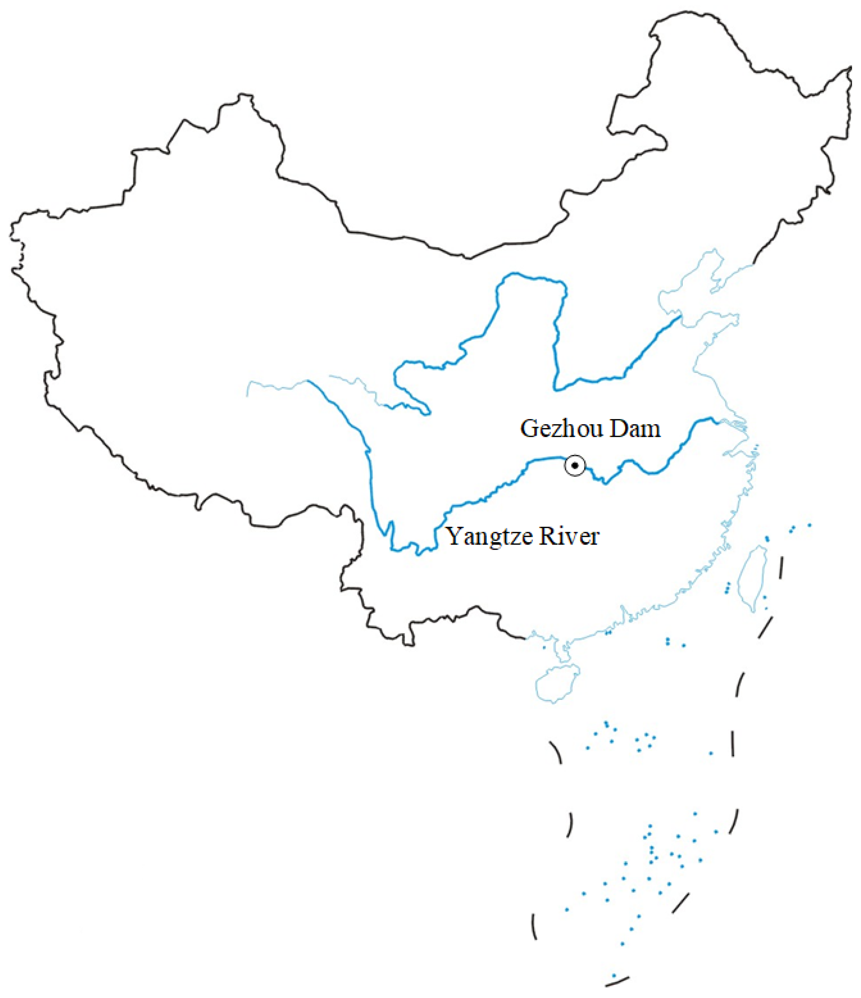
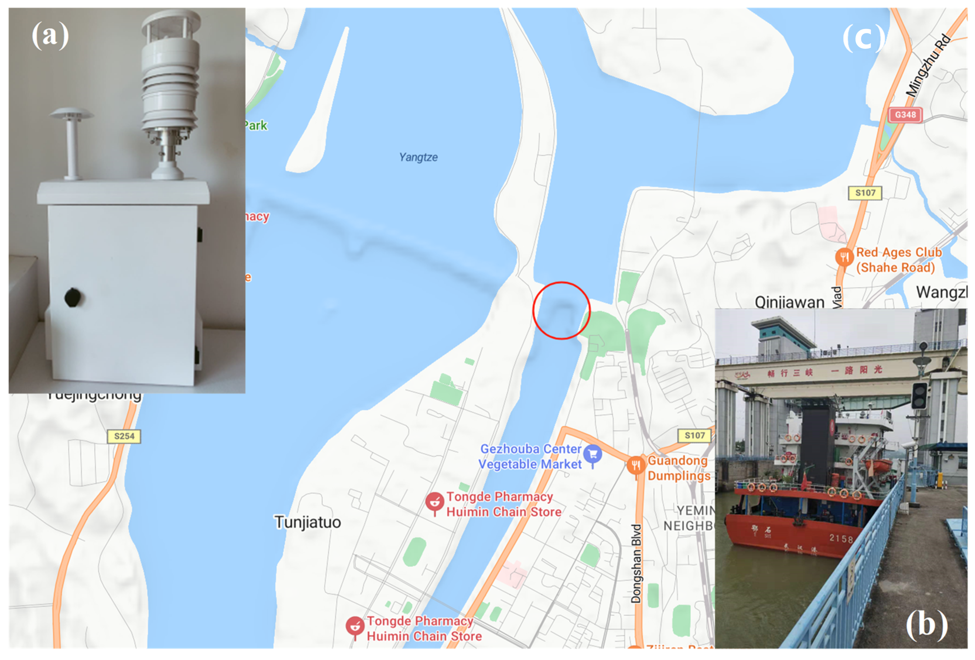
2.1. Instrumentation and Monitoring Location

Land-based monitoring was adopted in this study, and the monitoring location was the Gezhou Dam No. 3 lock in the middle reaches of the Yangtze River, the largest river in China (Figure 1). The sniffer monitoring equipment—which can measure the smoke plume of ships passing through the lock at a close distance—was installed on the Gezhou Dam No. 3 lock, China (Figure 2). The exhaust monitoring equipment included SO₂, CO₂, NO, and NO₂ gas sensors, PM_2.5 and PM₁₀ particulate matter sensors, as well as wind speed, wind direction, temperature, humidity, and pressure sensors. Considering the lower emissions of river vessels, the range of sensors used was more extensive than that typically used to monitor sea vessels. The principle and main parameters of the sensors are shown in

Table 1. Device sensor parameters.

Sensor	Principle	Effective Detection Range	Accuracy
SO2	Electrochemistry	0–1 ppm	≤±10 ppb
CO2	Non-dispersive infrared analyzer	0–1000 ppm	≤±5 ppm
NO2	Electrochemistry	0–1 ppm	≤±10 ppb
NO	Electrochemistry	0–1 ppm	≤±10 ppb
PM2.5	Laser scattering	0–1.0 mg/m3	≤±1%
PM10	Laser scattering	0–10 mg/m3	≤±1%

. The soft and hard technology and related technical details of this equipment have been demonstrated in detail in previous and proven to be an effective and feasible means for monitoring ship exhaust gas [5,33,34].

Gezhou Dam is the first large-scale hydropower station on the Yangtze River and the largest low-head, large-discharge, run-off hydropower station in the world. Ships passing through the dam area are required to lift/lower through the lock before navigation. Our equipment was installed above the No. 3 lock (Figure 2b,c); as the ships passed through this position, the positive sign of the exhaust was measured. Since the calculation of the EFs involves the difference between the measured value and the background value, the error of the sensor can be offset to a certain extent. In addition, it can be seen from Figure 2b that the monitoring position is very close to the ship below, approximately 10 m away. This is about as close as land-based monitoring can be positioned to the ship’s chimney mouth. By measuring in this way, the data obtained by the monitoring equipment in this study are less interfered with by environmental factors. This is not only conducive to obtaining effective measurement data but also to testing the actual measurement effect of the sniffer method.

2.2. Calculation of EF and FSC

Our equipment measured gas/particulate concentrations in the air continuously for 24 h. Only one ship could pass through the lock at a time, allowing the monitoring equipment to measure the ship’s exhaust as it passed. The navigation speed when entering or exiting a lock must not exceed 1.0 m/s, which indicates that the vessels inspected in this study are in the maneuvering phase; it generally took 20 min for ships to pass through the lock; the approximate time for ships to pass through the gate was obtained by combining it with the Automatic Identification System (AIS) data. In this way, we screened the smoke plume measurement dataset from the overall data collected by the equipment. Due to the low emissions from IRSs, some of the measured values were extremely weak, making it difficult to discern if they originated from the plume; therefore, we comprehensively considered the measured values of multiple sensors to determine the accurate time point or range of the measured plume values. The EF calculation formula was then used to calculate the data. Fuel-based EFs were calculated using the carbon balance method. ER_X (emission ratio) is defined as a ratio of the excess concentration of X emitted from a source divided by the excess concentration of CO₂ emitted by the source, as represented in Equation (1):

$${ER}_X={\displaystyle \frac{X_{peak}-X_{bg}}{{CO}_{2,peak}-{CO}_{2,bg}}}={\displaystyle \frac{\mathsf{\Delta }X}{\mathsf{\Delta }{CO}_2}}$$

(1)

where X_peak is the peak measure value of the gaseous (SO₂, NO, and NO₂) or mass concentration (PM_2.5 and PM₁₀); CO_2,peak is the CO₂; and X_bg and CO_2,bg are the background concentrations. Considering that the response times of various sensors were not consistent, we applied integral measurement values. The gases were measured in ppm, and the PM concentration was measured in μg m⁻³. The EF, EF_X (g kg⁻¹), was the amount of compound X released per amount of fuel burned and can be expressed using Equation (2):

$${EF}_X=\left\{\begin{array}{c}{ER}_X\times {\displaystyle \frac{M_X}{M_{{CO}_2}}}\times {EF}_{{CO}_2},for{SO}_2,NO,{NO}_2\hfill \\ {ER}_{PM}{EF}_{{CO}_2},for{PM}_{2.5},{PM}_{10}\hfill \end{array}\right.$$

(2)

where M_X and M_CO2 are the mole masses of the gases X and CO₂, respectively; and EF_CO2 is the EF of the reference species CO₂. We used a value of 3107 (g kg⁻¹) burned (Petzold et al., 2008) [35]. In addition, the FSC was calculated using Equation (3):

$$FSC={\displaystyle \frac{S\left(kg\right)}{fuel\left(kg\right)}}={\displaystyle \frac{{(SO}_{2,peak}-{SO}_{2,bg})\times A(S)}{{(CO}_{2,peak}-{CO}_{2,bg})\times A(C)}}\times 87(\%)=EF(S{O}_2)/20$$

(3)

where A(S) is the atomic weight of sulfur; and A(C) is the atomic weight of carbon. Thus, the FSC can be converted according to the SO₂ EF.

For real-time data monitored using the sniffer device, we used the package PeakUtils 1.3.3 in the Python programming language to identify the peak region in Equation (1) to calculate ER_X. According to the sensor accuracy information in Table 1, the difference between the peak value and the background value of a certain gas or PM must be greater than the accuracy of the corresponding sensor to obtain the valid peak area. For example, for CO₂, the peak area was considered valid only if the difference between the peak and the background value was more than 30 ppm. The most difficult aspect of measuring ship plumes is the low emissions of IRSs. Although we installed monitoring equipment at the location of the lock, we were able to quickly measure the emissions of passing ships at a relatively close distance. Nevertheless, it remains difficult to measure all or part of the effective gas/particulate matter as each ship passes through the lock. Therefore, during data processing, we compared the smoke plume data for various sensors, located the time point of the smoke plume measurement via detection of the peak values of multiple measurements, and applied this time point as the peak value of gas measurement data when calculating the EFs. Moreover, to avoid the influence of systematic error or environmental factors, the measured values of continuous 3-second effective peak values were selected, and the average value was considered the EF. In addition, due to the low emissions from IRSs, the peak region used in Equation (1) can be determined using the joint judgment of multiple sensor measurements. However, some measurements may be too low to be used for EF calculations. For example, while the NO and NO₂ values fell within the peak area, no such peak was observed for SO₂ due to the low sulfur content in the diesel used. Hence, this formula cannot calculate the EF of SO₂.

2.3. Ship Emission Estimate

In the process of compiling the ship emission inventories, the calculation process for emissions of individual ships is as follows:

$$E=E_{ME}+E_{AE}+E_{Boiler}$$

(4)

where E_ME, E_AE, and E_Boile represent the emissions from the main engines, auxiliary engines, and boiler, respectively. The method of compiling an emission inventory based on EFs can be divided into a fuel-based and power-based method. The power-based calculation method for main engines is as follows:

$$E_{ME}=MCR\times LF\times t\times \delta \times {EF}_{power}$$

(5)

where EF_power is the power-based EF (in units of g/kWh), which is usually obtained from ship emission factor databases, such as the Environmental Protection Agency (EPA) database; t is the duration. Then, the calculation formula for the engine load LF (dimensionless unit) is outlined below:

$$LF={\displaystyle \frac{P_{ME}}{MCR}}={\left(V/V_{Max}\right)}^3$$

(6)

where MCR is the maximum continuous power rating of the engine and V_Max is the maximum design speed of the ship—these parameters, along with the type of engine, can be obtained from classification societies, shipping companies, or maritime authorities. V is the ship’s real-time speed, extracted from AIS information; δ is a correction factor for low-load operation (normal load operation is 1), to reflect the ship’s real operating condition. Despite this, EF_power is not measured data, which may be a major source of uncertainty in the emission inventory compilation process; however, δ×EF_power can be converted to EF_fuel (fuel-based EF, in units of g/kg) as follows:

$$\delta \times {EF}_{power}=SFOC{\times EF}_{fuel}$$

(7)

where SFOC is the fuel consumption rate per kilowatt (in units of kg/kWh) per unit of time, which can be calculated from the engine load and type (Moreno-Gutierrez and Duran-Grados, 2021). Then, Formula (5) can be written as outlined below:

$$E_{ME}=MCR\times LF\times t\times SFOC\times {EF}_{fuel}=P_{ME}\times t\times SFOC\times {EF}_{fuel}=FC\times {EF}_{fuel}$$

(8)

where FC represents fuel consumption. Therefore, compiling emission inventories derived from power-based and fuel-based EFs is consistent in principle. The main difference lies in that the fuel-based EF used in this research was obtained through on site measurements, thus providing a more accurate estimate of ship emissions.

2.4. Uncertainties

In this study, the sniffer method was used to measure the exhaust gas of ships passing through the lock. Previously, we used this technology to conduct many studies on ship emissions based on UAV and land-based monitoring points and built a ship exhaust monitoring network system. Although this is a mature method, previous studies mainly measured the smoke plumes of OGVs; the emission intensity of IRSs was lower, which caused more uncertainties in the monitoring process. The main uncertainties of UAV measurements were summarized as sensor, measurement, calculation, and exhaust uncertainties.

The sensors used were purchased from Shenzhen Singoan Electronic Technology Co., Ltd., Shenzhen, China. Regarding sensor uncertainty, if the nonlinearity of two sensors is no more than ±1%, the linear error is negligible. Sensors were corrected via frequent calibrations with standard gases every month, and a quality management system comprising sensor linearity, sensitivity, repeatability, hysteresis, resolution, stability, drift, and other attributes of the minimum requirements was gradually established. Additionally, since the detection of particulate matter relies on the principle of laser scattering, calibration necessitates a complex experimental setup. Consequently, the sensors are generally not calibrated but are replaced on a periodic basis according to usage, typically ranging from six months to a year. Measurement uncertainty is mainly attributable to inadequate sampling, that is, the monitoring device was not placed in the plume to measure the gas concentration. Any sample that is not taken in the plume will face this uncertainty to a greater or lesser extent. In this study, the sampling point we selected is very close to the ship’s chimney, as shown in Figure 2, and is almost the closest position where land-based monitoring methods can be placed. However, due to the low concentrations emitted by IRSs, not all IRSs passing through were able to provide valid gas concentration measurements. Calculation uncertainty lies in selecting the background and peak values of gases and PM. Based on the AIS information, we can obtain the accurate time range of the ship passing under the equipment, and then select the calculated value according to the change trend of the measured gas concentration value. As shown in Equations (1)–(3), the measured values of continuous 3-second effective peak values were selected, and the average value was considered the EF. Exhaust uncertainty arises because the emitted gases or PM will undergo physical processes and chemical reactions in the ambient air, which are dynamic processes. The position of our monitoring equipment was very close to the chimney mouth, and the measured values obtained represent the emission characteristics of gas and particulate matter when the plume was recently discharged.

In any case, these uncertainties will occur during the measurement process. Specifically, uncertainties may vary depending on the environment and ship engine types, the type of fuel used, and the operating conditions. In the study by Beecken et al. (2014), the uncertainties for mass-based emission factors were 20% for SO and 24% for NOx [27]. Alfoldy et al. (2013) reported similar uncertainties of 23% for SO₂ and 26% for NOx [36]. J. Beeckeny et al. (2015) indicated that particulate matter was likely underestimated by about 30% [37]. The measurements in this study were taken from inland river ships, which have lower emissions, hence the uncertainties may be even greater. Therefore, we developed a QA/QC protocol regarding measurements with the monitoring equipment, which was implemented approximately as follows: we randomly sampled all the data in the dataset and automatically calculated the emission factor results of the gas and particulate matter using the calculation method described in Section 2.2. The measured data and calculated results were then evaluated manually by experienced experimenters to determine whether the sample was suitable for the calculation of EFs. Then, each step in the calculation model was optimized, and the sample results obtained by random sampling after multiple adjustments were consistent with the human calculation.

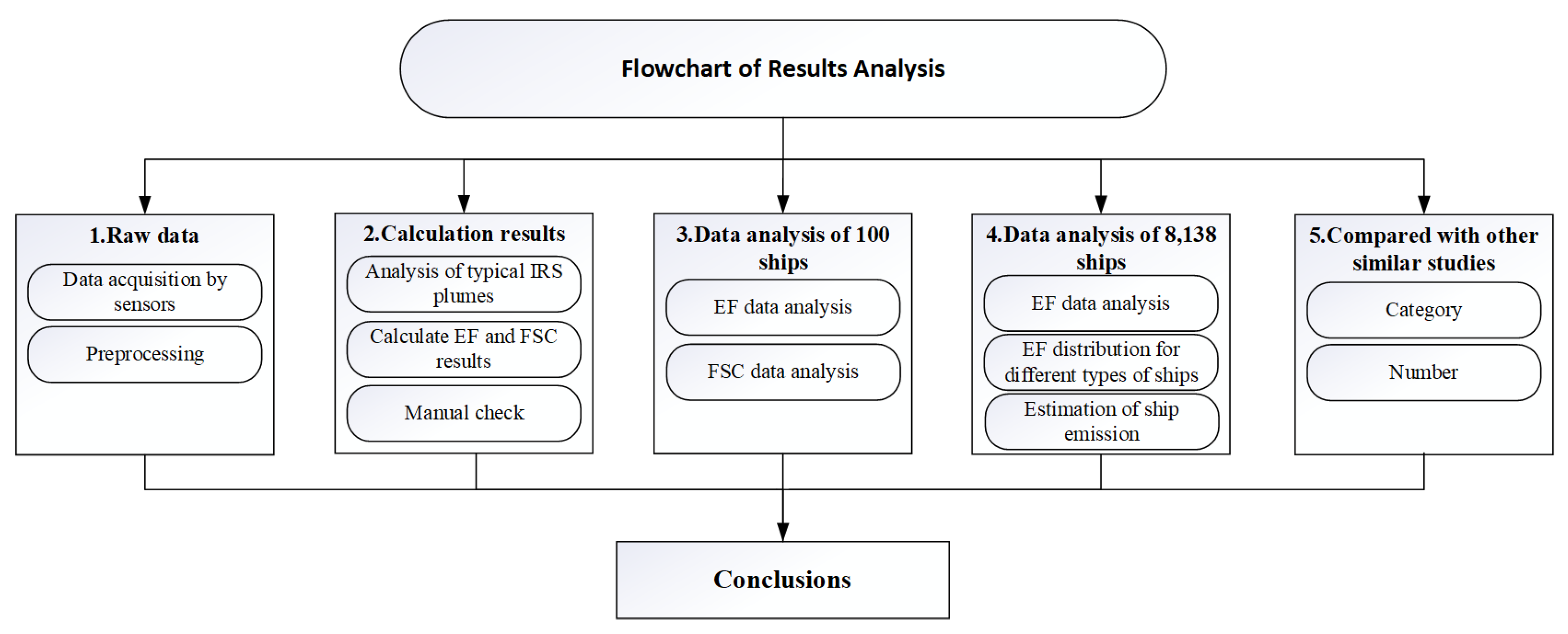
3. Results

In the monitoring campaign, the equipment described in Section 2.1 was utilized to monitor the inland river ships (IRSs) passing through the Gezhouba Dam No. 3 lock in Yichang, China, in order to collect the raw data and perform preliminary data processing. By analyzing typical IRS plume characteristics and selecting usable data, we then followed the methods outlined in Section 2.2 to calculate the fuel consumption coefficient (FSC) and emission factors (EFs) for polluting gases and particulate matter (PM). Finally, the calculated results were manually screened to verify the accuracy of the outcomes. A total of 8238 IRSs were monitored, which were mainly divided into two parts: From August 2020 to April 2021, we monitored the plumes from 100 ships in partnership with the maritime department for boarding and extracting oil samples to detect their FSC values. We determined that the FSC obtained by directly collecting and analyzing these oil samples represented the actual FSC values. From June 2021 to June 2022, we obtained monitoring data for 8138 ships, and only their plume contents were measured. Therefore, the following analyses were performed for two groups: one involving 100 ships and the other involving 8138 ships. The specific process is depicted in Figure 3.

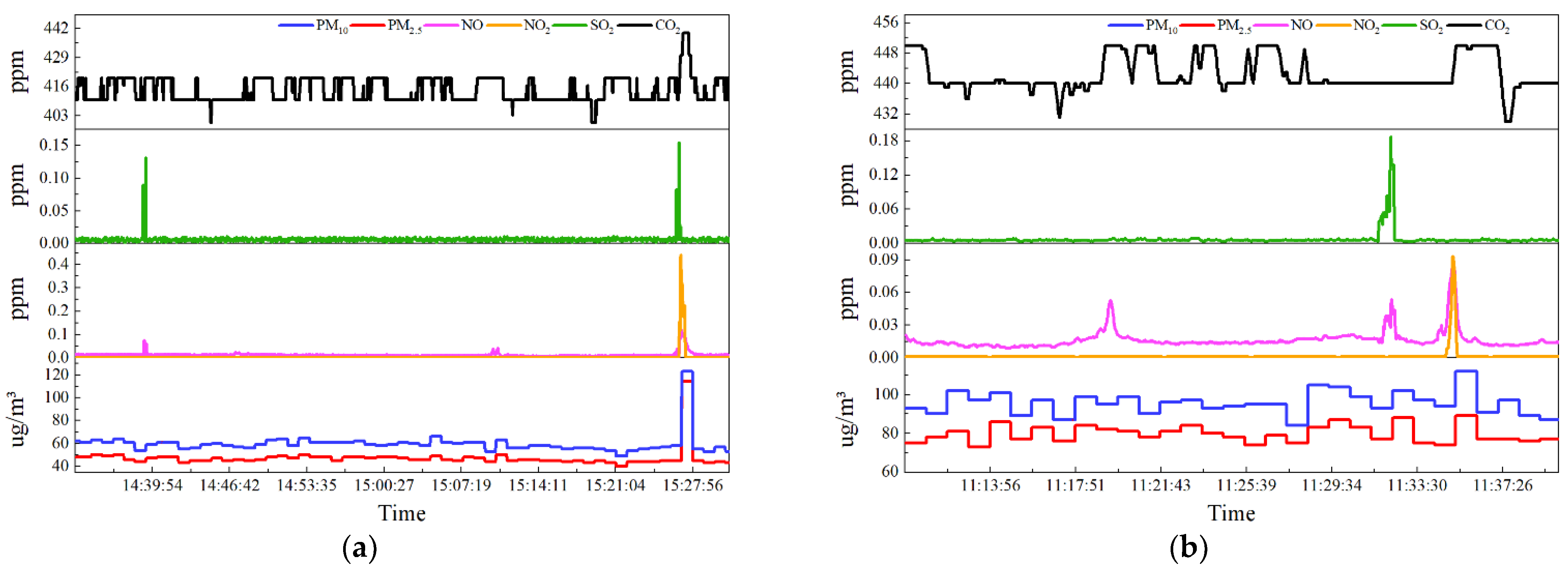
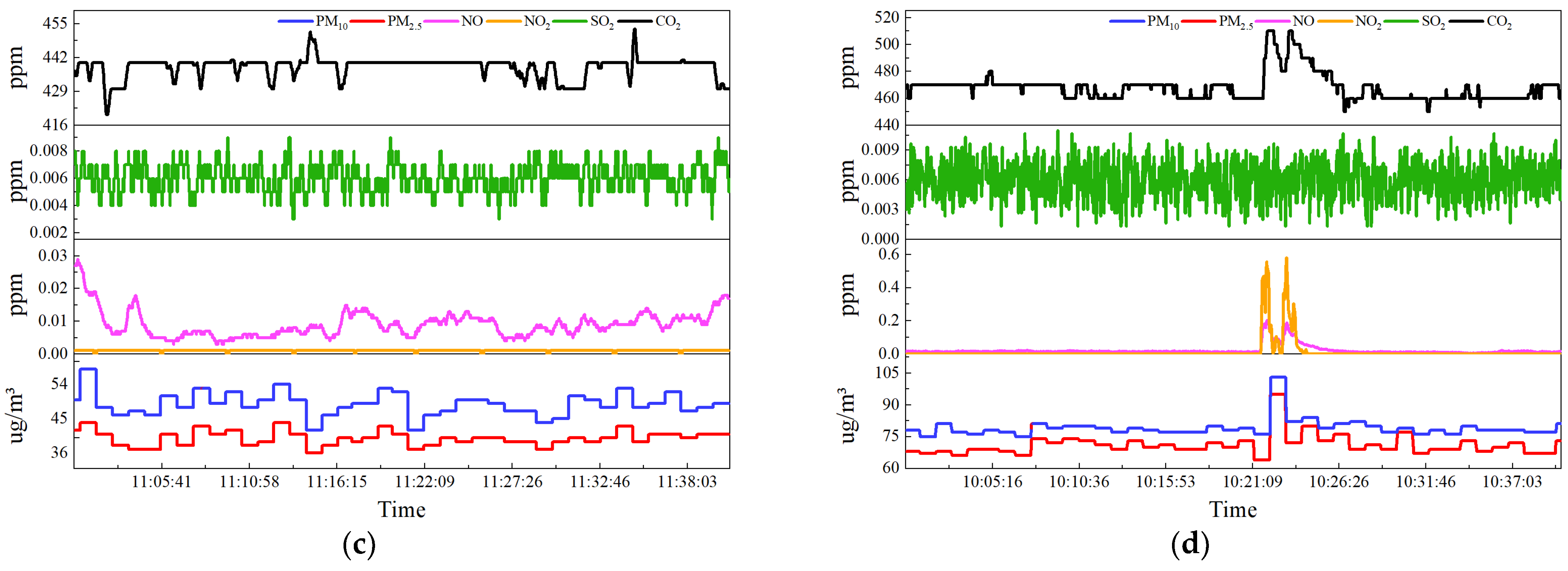
3.1. Typical IRS Plumes

To demonstrate the characteristics of gas/particulate matter measurements of IRSs monitored using the sniffer method, we selected four typical sets of data (Figure 4). CO₂, SO₂, NO, NO₂, PM_2.5, and PM₁₀ all exhibited obvious peak areas around 15:27:00; therefore, this set of data was used to calculate the EFs of SO₂, NO, NO₂, PM_2.5, and PM₁₀ (Figure 2a). Meanwhile, in Figure 4b, NO, NO₂, PM_2.5, and PM₁₀ exhibit obvious peak areas; however, the associated time points are relatively offset. Moreover, there was no obvious peak value in the CO₂ measurement series, and the fluctuation range was small, ranging from 430 ppm to 450 ppm; hence, this dataset could not be used to calculate EFs. According to Equation (2), the difference between the peak CO₂ value and the background value is the denominator. Thus, if the numerator value is fixed, a small denominator can lead to a large EF result, which deviates from the actual situation. Therefore, to calculate the EFs, it was necessary to measure the peak area of obvious CO₂ values. In Figure 4c, CO₂, SO₂, NO, NO₂, PM_2.5, and PM₁₀ have no obvious peaks, which may be due to the low emissions from ships or other environmental factors. Regardless, the measured values were too low, and the associated dataset could not be applied to calculate EFs. In contrast, within Figure 4d, CO₂, NO, NO₂, PM_2.5, and PM₁₀ all have obvious peaks, which can be used to calculate EFs; however, no obvious peak value is observed in the SO₂ measurement, which might be due to the low sulfur content in the fuel oil used by the ship and the low SO₂ concentration in the exhaust gas. Therefore, this dataset was not used to calculate the EF of SO₂.

By analyzing the above four datasets, it was apparent that the IRS emissions were low, making the measurement of the smoke plumes more difficult. Although analysis of the measured values for multiple sensors could determine the peak time point of the measured values, the effective EF calculation results were attainable only when an obvious synchronous peak area was observed between the measured values of a certain gas/particulate matter and the measured values of CO₂. The analysis of these four types of typical data shows that, although plume measurements can be obtained while the ship is passing, only some of the data can be successfully used to estimate the EF and FSC.

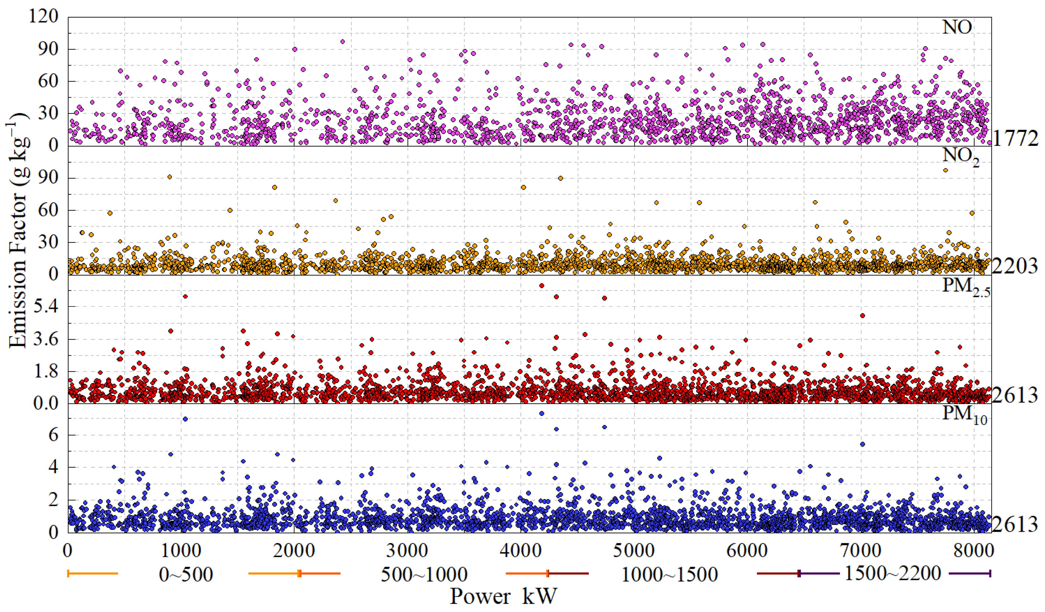
3.2. EF Estimation of 100 Ships

Due to the low emissions from IRSs, only a portion of the data from the 100 boarded ships were calculated to obtain the EFs for SO₂, NO, NO₂, PM_2.5, and PM₁₀ (Figure 4). Only 12 groups of SO₂ EFs were calculated, primarily due to the low FSC and SO₂ concentrations in emissions in accordance with the ECA policy of the Chinese government. As a result, effective monitoring data were only obtained in a small number of cases by using the sniffer method. The EFs of NO were measured in 28 datasets and ranged from 3.37 to 46.74 g kg⁻¹ (average: 20.02 ± 13.17 g kg⁻¹). The EFs of NO₂ were measured in 37 datasets and ranged from 3.37 to 32.80 g kg⁻¹ (average: 8.37 ± 5.25 g kg⁻¹). The EF detection rate of NO₂ was higher than that of NO, primarily because NO is easily oxidized to NO₂ at room temperature, resulting in low NO concentrations in some cases, which could not be applied to calculate NO levels. A total of 39 datasets measured PM_2.5 and PM₁₀ EFs, ranging from 0.05 to 3.19 g kg⁻¹ (average of 1.02 ± 0.80 g kg⁻¹) and 0.05 to 3.19 g kg⁻¹ (average: 1.09 ± 0.81 g kg⁻¹), respectively. Both PM_2.5 and PM₁₀ were detected in the fuel from the same ship, as PM₁₀ contains PM_2.5 particles. Meanwhile, the EF value of PM₁₀ was similar to that of PM_2.5, indicating that the main PM emitted by the ships was smaller than 2.5 μm, which is consistent with previous monitoring conclusions [17,31]. Overall, the detection rates of pollution gas and PM from ships were lower than 50%, indicating that obtaining exhaust gas measurements of IRSs is difficult with these low detection rates. Meanwhile, the power range of all ships ranged from 176 kW to 1942 kW (Figure 5). Within this range, the power level and EF results exhibited no apparent statistical relationships. In addition, some ships did not have any valid EF results, indicating that the sniffer equipment provided no valid gas or PM measurements.

3.3. Comparing the Estimated FSC with the Actual FSC

We then converted the SO₂ EF results into FSCs and compared them with the actual FSC values of the oil samples. The results show that the actual FSC value for ship target No. 2 was 118.94 ppm, while the estimated FSC value was 109.74 ppm, with an ~10 ppm deviation (

Table 2. Actual FSC, estimated FSC, and estimated EF(SO₂) values of ships.

ID	EF-Estimated Value (g kg−1)	FSC-Estimated Value (ppm)	FSC Actual Value (ppm)
1	69.41	34.70	10.93
2	237.88	118.94	108.74
3	113.74	56.87	7.87
4	167.33	83.66	3.69
5	30.36	15.18	8.42
6	17.40	8.70	3.54
7	50.33	25.17	9.95
8	0.78	0.39	9.59
9	0.72	0.36	9.62
10	35.96	17.98	7.61
11	9.55	4.77	8.98
12	48.46	24.23	10.09

), which is considerably smaller than the previously reported 300 ppm deviation [5]. Meanwhile, for all other ships, the actual FSC values were <11 ppm, whereas the estimated FSC values ranged from 0.36 to 83.66 ppm. Collectively, these results suggest that the sniffer method is relatively accurate when measuring levels >100 ppm. However, when the FSC is <100 ppm, the results become significantly skewed due to the relatively low FSC. Hence, with a diesel sulfur limit of 10 ppm, it may be difficult to accurately judge compliance with ship targets using the sniffer method.

3.4. EF Estimation of 8138 Ships

According to the comparative analysis presented in Section 3.1, the calculated SO₂ EF and FSC results markedly differed from the actual values. Therefore, only EFs for NO, NO₂, PM_2.5, and PM₁₀ were calculated in the monitoring data for the 8138 ships (Figure 6). The power range of the ship engines was 140–2131 kW, whereas the EFs for NO, NO₂, PM_2.5, and PM₁₀ were detected in 1772 (21.77%), 2203 (27.07%), 2613 (32.11%), and 2613 (32.11%) of the ships, respectively. The associated EF values were 24.02 ± 16.92 g kg⁻¹, 10.30 ± 8.08 g kg⁻¹, 0.72 ± 0.60 g kg⁻¹, and 0.92 ± 0.70 g kg⁻¹, respectively. By comparing the monitoring results of 100 ships, the EF results from 8138 ships displayed little difference. If the test results for the 100 ships were considered as the sampling group, those for the 8138 ships were considered as the population. It was apparent that the mean and mean square error calculated for the sample did not differ significantly from the mean and mean square error of the population, which conforms to the law of large numbers.

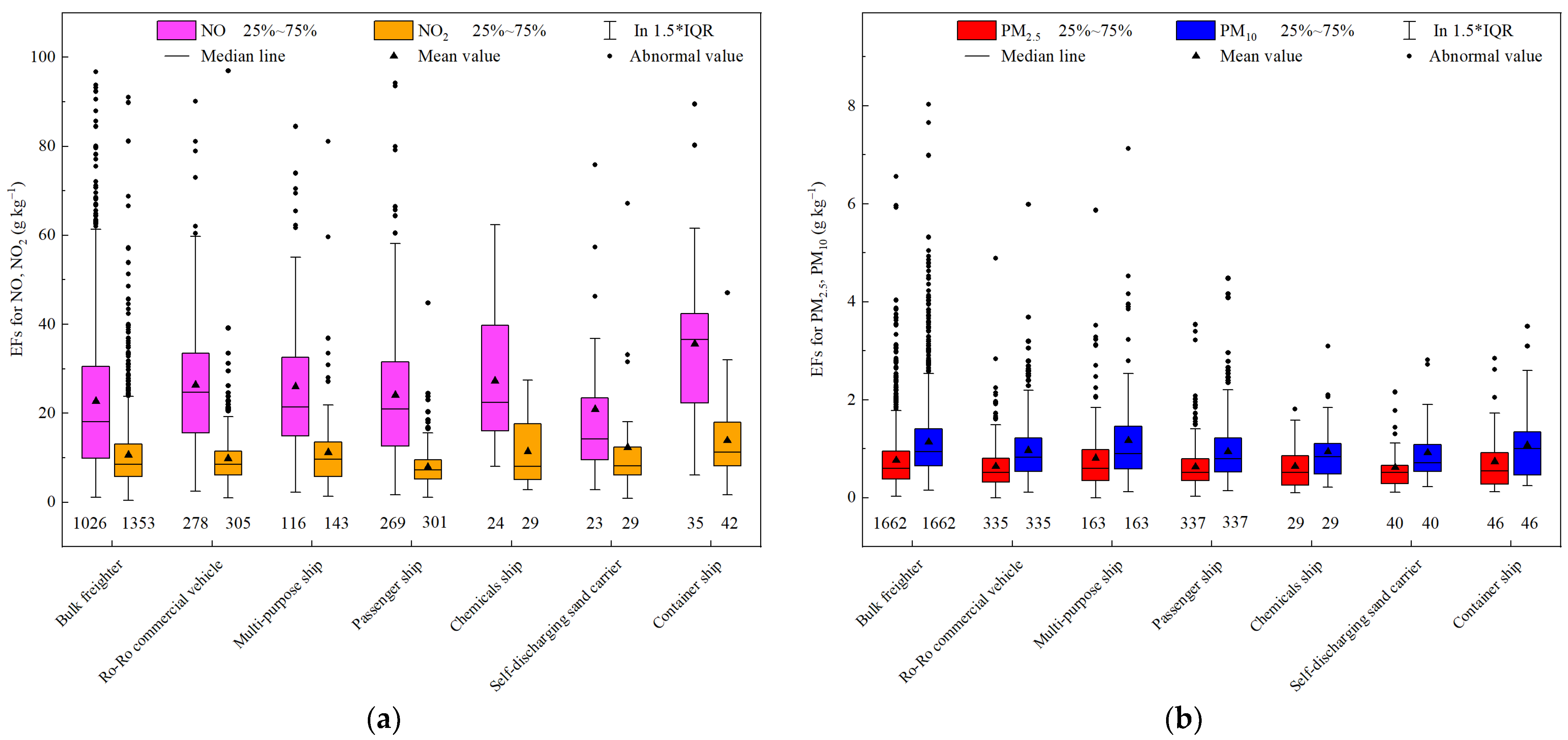
3.5. EF Distributions for Different Types of Ships

According to the maritime department’s ship registration information, ship types were divided into seven categories: Bulk freighter, Ro-Ro commercial vehicle, Multi-purpose ship, Passenger ship, Chemicals ship, Self-discharging sand carrier, and Container ship; the EFs of NO, NO₂, PM_2.5, and PM₁₀ were calculated for each (Figure 7). To avoid the influence of abnormal data, we generated modified box plots, that is, the difference between the first and fourth scores, Q1, and the third and fourth scores, Q3, were applied as the interquartile range (IQR) for the EF results of various ship types. If the value was <Q1−1.5×IQR or >Q3+1.5×IQR, it was considered an outlier and indicated as such in the figure. In terms of nitrogen oxides, the NO and NO₂ EFs of the Container ship were higher than those of the other types of ships, followed by the Chemicals ship type. In terms of PM, the Multi-purpose ship had the highest PM_2.5 EF, while the EFs of the other types of ships did not differ significantly. The EF for PM₁₀ was slightly higher than that of PM_2.5, further confirming that the PM emitted by all ship types was <2.5 μm. Although the NOx EF of the Container ship was higher than those of the other ships, generally, no significant differences were observed in the EFs of the various IRS types. This distinction was consistent with the research results of Burgard and Bria (2016) [38]. This might be caused by the fact that the types of monitored ships in the present study were all river ships. Although the types of ships were different, they all mainly used diesel engines. According to the boarding results of the 100 ships, most of the ships used qualified diesel oil. Moreover, the sailing state of the ship was at a low speed through the lock. As the ships’ engine type, fuel type, and sailing conditions were the same, the measured EFs were also similar.

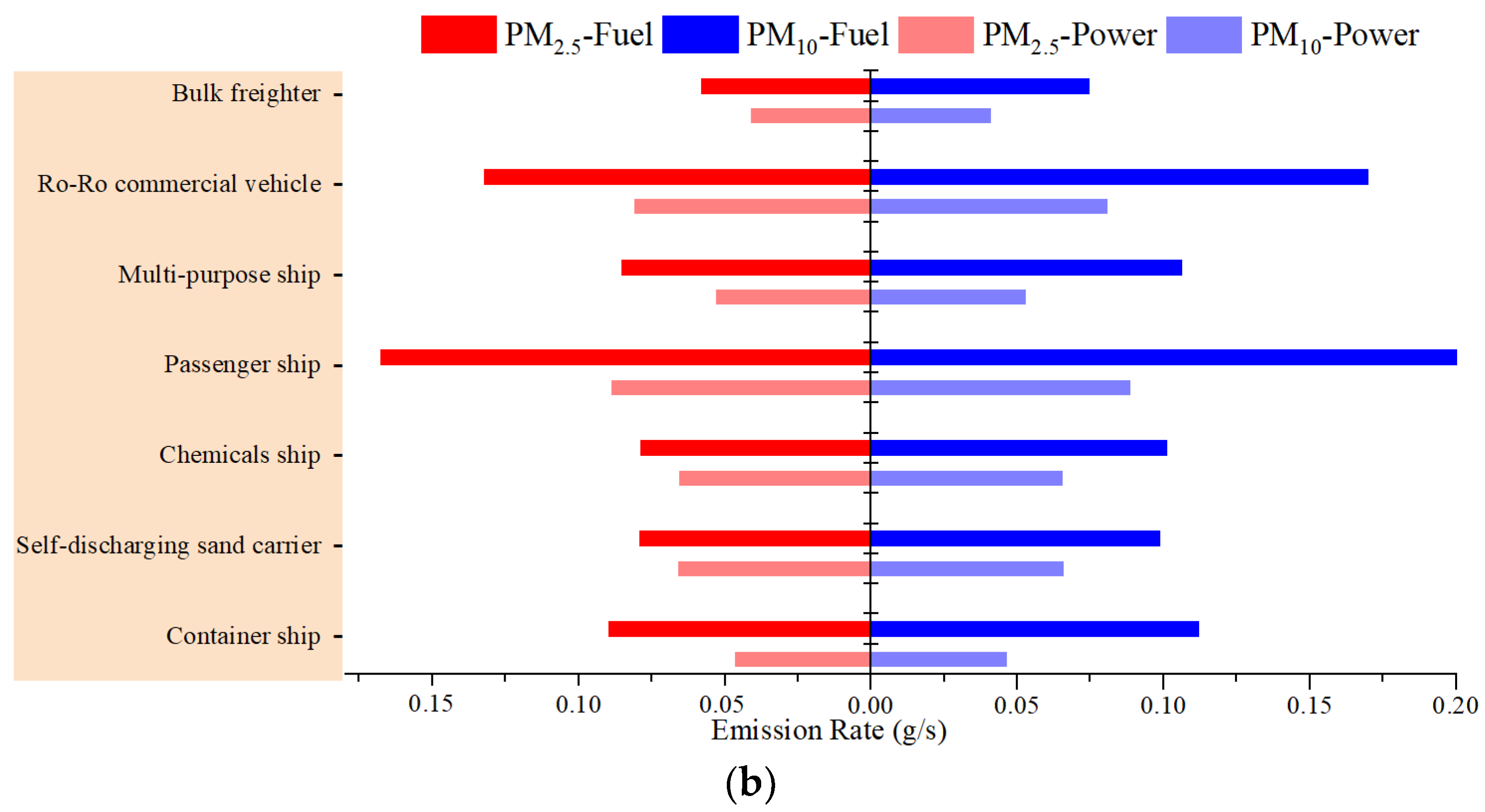
3.6. Estimation of Ship Emission

As shown in Figure 8, the instantaneous emissions (emission rate, unit is g/s) of these ships when they pass through the lock are estimated according to the measured EFs (fuel-based EFs), and the average emission rate calculated for the different types of ships is displayed. Meanwhile, we also used the power-based method mentioned in Section 2.3 to calculate the average emission rate of ships. The power-based EFs used are derived from the EPA (https://www.epa.gov/electronic-reporting-air-emissions/webfire, last access: 6 March 2023).

It can be seen that although there is no significant difference in the estimated emissions between the two methods for any type of ship, there is still a pattern of difference. The NOx emissions estimated based on the fuel method are comparatively lower, while the PM emissions estimated are relatively higher. Since the estimation is directly based on the measured EFs, the fuel-based method may be closer to the actual emissions of ships. The reason for the difference may be that the EFs from EPA are mainly from measurement experiments before 2019, while this study is based on measurements after 2019. Due to the reduction of the FSC, the EFs from earlier measurement experiments may no longer reflect the actual emissions of ships.

3.7. Comparison and Discussion

Our experimental results were compared with those of other similar monitoring studies performed over the past 20 years (Table 3). Two main types of measurements were reported for ship EFs: fuel-based and power-based. Given that the current study measured fuel-based emissions, only other fuel-based EFs are compared here. Among them, since the EF of SO₂ was significantly biased when employing the sniffer method, we applied the actual FSC values detected for the 100 ships to convert to SO₂ EFs. The value of No. 2 in Table 2 is considered as an exception and has been excluded. Meanwhile, NOx represented the combined NO and NO₂ values. However, the PM categories were not consistently defined across the studies, therefore, we have presented them separately.

In terms of quantity, this study includes 8,138 vessels, while the largest sample size in other studies only reaches 311 ships. It is evident that the scope of this study is extensive, covering a greater number of vessels than ever before in similar research, thus providing a solid data foundation for in-depth analysis. Moreover, the EF of SO₂ converted from the FSC is significantly lower than that of other studies. Overall, the EFs of SO₂, NOx, and PM exhibited downward trends over time. However, this conclusion may be insufficient because different studies have used various methods, regions, and fleet compositions without properly correcting for these differences. Moreover, some studies have suggested that NOx emissions may actually be increasing, which contradicts our conclusion. For instance, recent research [39] has reported an upward trend in NOx emissions. Therefore, we need to approach the trend of EF changes with caution and further explore the reasons for these differences in future studies. In spite of this, the comparison results show no significant difference between the EFs of the IRSs and OGVs. Indeed, the measurement times in the current study represent the most recent time point; all of the calculated results were lower than those reported in any other study. This suggests that in recent years, with attention being paid to ship emissions and the implementation of relevant policies, the EFs of ships have been reduced, likely resulting in a subsequent decrease in associated air pollution. At the same time, it can be observed from Table 3 that although OGVs are more powerful than IRSs and their emissions are generally higher, there is no significant difference in the value of NOx EFs, which are basically in the same order of magnitude. The SO₂ EF depends on the quality of fuel used, and the PM data are relatively small and may require more in-depth measurement and demonstration. In addition, as the sulfur content of fuel used by ships decreases, not all emissions show a downward trend, and relevant studies have shown that IVOCs and VOCs are on the rise [40,41,42].

Table 3. Comparison of research results with other studies.

	Year/Category/Number	SO2/g kg−1	NOx (NO+NO2)/g kg−1	PM/g kg−1
Corbett and Robinson, 2001 [43]	1999/IRS/1	/	70 ± 4.2	/
Sinha et al., 2003 [44]	2000/OGV/2	2.9 ± 0.2–52.2 ± 3.7	22.3 ± 1.1–65.5 ± 3.3	/
Williams et al., 2009 [45]	2006/OGV/>200	5.6 ± 8.8–48.1 ± 8.3	27.7 ± 8.2–87.0 ± 29.6	/
Fu et al., 2013 [21]	IRS/1	/	98.9	PM2.5: 3.2
Burgard and Bria, 2016 [38]	2009/OGV/16	24 ± 7–40 ± 5	60 ± 6–94 ± 27	/
Zhang et al., 2016 [22]	3	0.92–2.60	31.6 ± 2.20–115 ± 44.3	PM2.5: 0.16 ± 0.07–9.40 ± 2.13
Beecken et al., 2014 [27]	2011/OGV/158	18.8±6.5	66.6±23.4	/
Beecken et al., 2015 [37]	2011/OGV/311	4.6–18.2	58	/
Kurtenbach et al., 2016 [18]	2013/IRS/>170	/	54 ± 4	PM10: ≥2.0 ± 0.3
Betha et al., 2017 [32]	2014/OGV/1	/	47–64	PM10: 0.5–1.2
Liu et al., 2018 [46]	FS/8	/	48.6 ± 4.3–75.6 ± 7.5	PM2.5: 3.27 ± 0.3–20.9 ± 1.9
Xiao et al., 2019 [23]	IRS/5	0.08–5.50	36.36–48.61	PM2.5: 0.32–4.17
This work	2021/IRS/8138	0.01 ± 0.02	34.32 ± 25.00	PM2.5: 0.72 ± 0.60 PM10: 0.92 ± 0.70

Year refers to the time when vessel-emission-monitoring activities began; Category refers to whether the vessel is an inland river ship (IRS), ocean-going vessel (OGV), or fishing ship (FS); Number refers to the number of ships measured. A range of emission factor results indicates that the study measured different categories of ships. All results were measured in g kg⁻¹. Note: various results came from different sources so the accuracy of the resulting data is inconsistent.

Table 3. Comparison of research results with other studies.

	Year/Category/Number	SO2/g kg−1	NOx (NO+NO2)/g kg−1	PM/g kg−1
Corbett and Robinson, 2001 [43]	1999/IRS/1	/	70 ± 4.2	/
Sinha et al., 2003 [44]	2000/OGV/2	2.9 ± 0.2–52.2 ± 3.7	22.3 ± 1.1–65.5 ± 3.3	/
Williams et al., 2009 [45]	2006/OGV/>200	5.6 ± 8.8–48.1 ± 8.3	27.7 ± 8.2–87.0 ± 29.6	/
Fu et al., 2013 [21]	IRS/1	/	98.9	PM2.5: 3.2
Burgard and Bria, 2016 [38]	2009/OGV/16	24 ± 7–40 ± 5	60 ± 6–94 ± 27	/
Zhang et al., 2016 [22]	3	0.92–2.60	31.6 ± 2.20–115 ± 44.3	PM2.5: 0.16 ± 0.07–9.40 ± 2.13
Beecken et al., 2014 [27]	2011/OGV/158	18.8±6.5	66.6±23.4	/
Beecken et al., 2015 [37]	2011/OGV/311	4.6–18.2	58	/
Kurtenbach et al., 2016 [18]	2013/IRS/>170	/	54 ± 4	PM10: ≥2.0 ± 0.3
Betha et al., 2017 [32]	2014/OGV/1	/	47–64	PM10: 0.5–1.2
Liu et al., 2018 [46]	FS/8	/	48.6 ± 4.3–75.6 ± 7.5	PM2.5: 3.27 ± 0.3–20.9 ± 1.9
Xiao et al., 2019 [23]	IRS/5	0.08–5.50	36.36–48.61	PM2.5: 0.32–4.17
This work	2021/IRS/8138	0.01 ± 0.02	34.32 ± 25.00	PM2.5: 0.72 ± 0.60 PM10: 0.92 ± 0.70

Year refers to the time when vessel-emission-monitoring activities began; Category refers to whether the vessel is an inland river ship (IRS), ocean-going vessel (OGV), or fishing ship (FS); Number refers to the number of ships measured. A range of emission factor results indicates that the study measured different categories of ships. All results were measured in g kg⁻¹. Note: various results came from different sources so the accuracy of the resulting data is inconsistent.

4. Conclusions

Since the implementation of the MARPOL 73/78 International Convention for the Prevention of Pollution from Ships in 2005, numerous studies have been performed to monitor ship emissions. However, IMO limits on ship emissions have been primarily based on OGVs, with most relevant research focused on their emissions. Due to the low emissions from IRSs, obtaining accurate monitoring values is challenging using common equipment. In this study, land-based sniffer equipment was deployed in the Gezhou Dam No. 3 lock to monitor 8,238 ships passing through the lock at a close range. Among them, 100 ships were selected to provide oil samples to obtain actual FSCs. After data analysis and comparison with relevant studies, the following conclusions were made:

• The emissions of IRSs are low and associated monitoring is difficult. Under the restriction of 10 ppm FSC, processing of the samples collected from 100 ships revealed that most ships complied with the regulations, with an average FSC of 7.17 ± 10.90 ppm. However, the measured SO₂ data could not be accurately applied to calculate the effective SO₂ EF and the FSC. Meanwhile, the sniffer method was found to be effective at obtaining accurate results when the FSC exceeded 100 ppm;
• In the monitoring experiment of 8138 ships, the detection rates of NO, NO₂, PM_2.5, and PM₁₀ by the land-based sniffer were 21.77%, 27.07%, 32.11%, and 32.11%, respectively, and the results were 24.02 ± 16.92 g kg⁻¹, 10.30 ± 8.08 g kg⁻¹, 0.72 ± 0.60 g kg⁻¹, and 0.92 ± 0.70 g kg⁻¹, respectively. The monitored ship types were divided into seven categories, with the two categories producing the highest NO EFs being the Container ship category, followed by the Chemicals ship category. The PM EFs of the different ship types did not differ significantly;
• Estimates of the ship emissions during the passage through the lock were made based on the measured fuel-based EF. These results were compared with emission estimates using the power-based method, showing that the estimated NOx emissions based on fuel-based EFs were lower but PM emissions were higher, which may be closer to the actual emissions of ships;
• The conclusion of this paper indicates that, compared to the past, the emission factors (EFs) for SO₂, NOx, and PM have shown a downward trend; however, the comprehensiveness of this conclusion may be questioned as there are differences in methodology, regional selection, and fleet composition among the studies, and these differences have not been properly adjusted for.

In conclusion, in this study, we verified the practicability of the sniffer method and provided a basis for understanding emissions from IRSs under the FSC constraint of 10 ppm, and estimated the emissions of IRSs based on these measured fuel-based EFs. However, this study has certain limitations. Although many ship plumes were measured, the EFs obtained were from the data measured when ships passed through the lock; thus, differences under different sailing states were not thoroughly studied. Furthermore, the real-time power data of these ships were not mastered. This means that the EFs measured by this study can only characterize the emission characteristics during low-speed navigation of ships. These limitations need to be overcome in follow-up monitoring studies to better understand the emission characteristics of IRSs and thus assess the effect of IRS emissions on the atmospheric environment and human health more accurately.

References

- Corbett, J. Shipping Emissions in East Asia. Nat. Clim. Chang. 2016, 6, 983–984. [Google Scholar] [CrossRef]
- Sofiev, M.; Winebrake, J.J.; Johansson, L.; Carr, E.W.; Prank, M.; Soares, J.; Vira, J.; Kouznetsov, R.; Jalkanen, J.-P.; Corbett, J.J. Cleaner Fuels for Ships Provide Public Health Benefits with Climate Tradeoffs. Nat. Commun. 2018, 9, 406. [Google Scholar] [CrossRef] [PubMed]
- MARPOL: International Convention for the Prevention of Pollution from Ships, 1973 as modifified by the Protocol of 1978–Annex VI: Prevention of Air Pollution from Ships; International Maritime Organization (IMO): London, UK, 1997.
- Balzani Lööv, J.M.; Alfoldy, B.; Gast, L.F.L.; Hjorth, J.; Lagler, F.; Mellqvist, J.; Beecken, J.; Berg, N.; Duyzer, J.; Westrate, H.; et al. Field test of available methods to measure remotely SOx and NOx emissions from ships. Atmos. Meas. Tech. 2014, 7, 2597–2613. [Google Scholar] [CrossRef]
- Zhou, F.; Pan, S.; Chen, W.; Ni, X.; An, B. Monitoring of Compliance with Fuel Sulfur Content Regulations through Unmanned Aerial Vehicle (UAV) Measurements of Ship Emissions. Atmos. Meas. Tech. 2019, 12, 6113–6124. [Google Scholar] [CrossRef]
- Liu, H.; Fu, M.; Jin, X.; Shang, Y.; Shindell, D.; Faluvegi, G.; Shindell, C.; He, K. Health and Climate Impacts of Ocean-Going Vessels in East Asia. Nat. Clim. Chang. 2016, 6, 1037–1041. [Google Scholar] [CrossRef]
- Weng, J.; Shi, K.; Gan, X.; Li, G.; Huang, Z. Ship Emission Estimation with High Spatial-Temporal Resolution in the Yangtze River Estuary Using AIS Data. J. Clean. Prod. 2020, 248, 119297. [Google Scholar] [CrossRef]
- Moreno-Gutiérrez, J.; Durán-Grados, V. Calculating Ships’ Real Emissions of Pollutants and Greenhouse Gases: Towards Zero Uncertainties. Sci. Total Environ. 2021, 750, 141471. [Google Scholar] [CrossRef]
- Lack, D.A.; Cappa, C.D.; Langridge, J.; Bahreini, R.; Buffaloe, G.; Brock, C.; Cerully, K.; Coffman, D.; Hayden, K.; Holloway, J.; et al. Impact of Fuel Quality Regulation and Speed Reductions on Shipping Emissions: Implications for Climate and Air Quality. Environ. Sci. Technol. 2011, 45, 9052–9060. [Google Scholar] [CrossRef] [PubMed]
- Tao, L.; Fairley, D.; Kleeman, M.J.; Harley, R.A. Effects of Switching to Lower Sulfur Marine Fuel Oil on Air Quality in the San Francisco Bay Area. Environ. Sci. Technol. 2013, 47, 10171–10178. [Google Scholar] [CrossRef]
- Wan, Z.; Zhu, M.; Chen, S.; Sperling, D. Pollution: Three Steps to a Green Shipping Industry. Nature 2016, 530, 275–277. [Google Scholar] [CrossRef]
- Fan, S.; Liu, C.; Xie, Z.; Dong, Y.; Hu, Q.; Fan, G.; Chen, Z.; Zhang, T.; Duan, J.; Zhang, P.; et al. Scanning Vertical Distributions of Typical Aerosols along the Yangtze River Using Elastic Lidar. Sci. Total Environ. 2018, 628–629, 631–641. [Google Scholar] [CrossRef] [PubMed]
- Feng, J.; Zhang, Y.; Li, S.; Mao, J.; Patton, A.P.; Zhou, Y.; Ma, W.; Liu, C.; Kan, H.; Huang, C.; et al. The Influence of Spatiality on Shipping Emissions, Air Quality and Potential Human Exposure in the Yangtze River Delta/Shanghai, China. Atmos. Chem. Phys. 2019, 19, 6167–6183. [Google Scholar] [CrossRef]
- Ni, P.; Wang, X.; Li, H. A Review on Regulations, Current Status, Effects and Reduction Strategies of Emissions for Marine Diesel Engines. Fuel 2020, 279, 118477. [Google Scholar] [CrossRef]
- Huang, C.; Hu, Q.; Li, Y.; Tian, J.; Ma, Y.; Zhao, Y.; Feng, J.; An, J.; Qiao, L.; Wang, H.; et al. Intermediate Volatility Organic Compound Emissions from a Large Cargo Vessel Operated under Real-World Conditions. Environ. Sci. Technol. 2018, 52, 12934–12942. [Google Scholar] [CrossRef]
- Liu, Z.; Chen, Y.; Zhang, Y.; Zhang, F.; Feng, Y.; Zheng, M.; Li, Q.; Chen, J. Emission Characteristics and Formation Pathways of Intermediate Volatile Organic Compounds from Ocean-Going Vessels: Comparison of Engine Conditions and Fuel Types. Environ. Sci. Technol. 2022, 56, 12917–12925. [Google Scholar] [CrossRef]
- Keuken, M.P.; Moerman, M.; Jonkers, J.; Hulskotte, J.; Denier Van Der Gon, H.A.C.; Hoek, G.; Sokhi, R.S. Impact of Inland Shipping Emissions on Elemental Carbon Concentrations near Waterways in The Netherlands. Atmos. Environ. 2014, 95, 1–9. [Google Scholar] [CrossRef]
- Kurtenbach, R.; Vaupel, K.; Kleffmann, J.; Klenk, U.; Schmidt, E.; Wiesen, P. Emissions of NO, NO2 and PM from inland shipping. Atmos. Chem. Phys. 2016, 16, 14285–14295. [Google Scholar] [CrossRef]
- MOT. Implementation of the Ship Emission Control Area in Pearl River Delta, the Yangtze River Delta and the Bohai Rim (Beijing–Tianjin–Hebei Area); China Ministry of Transport: Beijing, China, 2015. Available online: http://www.gov.cn/xinwen/2015-12/04/content_5019932.htm (accessed on 1 November 2022).
- MOT. Implementation Scheme of the Domestic Emission Control Areas for Atmospheric Pollution from Vessels; China Ministry of Transport: Beijing, China, 2018. Available online: https://www.msa.gov.cn/public/documents/document/mte1/odi2/~edisp/20190124115826051.pdf (accessed on 1 November 2022).
- Fu, M.; Ding, Y.; Ge, Y.; Yu, L.; Yin, H.; Ye, W.; Liang, B. Real-World Emissions of Inland Ships on the Grand Canal, China. Atmos. Environ. 2013, 81, 222–229. [Google Scholar] [CrossRef]
- Zhang, F.; Chen, Y.; Tian, C.; Lou, D.; Li, J.; Zhang, G.; Matthias, V. Emission Factors for Gaseous and Particulate Pollutants from Offshore Diesel Engine Vessels in China. Atmos. Chem. Phys. 2016, 16, 6319–6334. [Google Scholar] [CrossRef]
- Xiao, X.; Li, C.; Ye, X. Emission characteristics of gas- and particle- phase pollutants from river vessels in cruising mode. Acta Sci. Circumstantiae 2019, 39, 13–24. [Google Scholar] [CrossRef]
- Cao, Y.; Zhang, W.; Wang, X.; Wu, L.; Qian, G. The Relationship between Atmospheric Pollutant Emissions and Fuel Qualities of Inland Vessels in Jiangsu Province, China. J. Air Waste Manag. Assoc. 2019, 69, 305–312. [Google Scholar] [CrossRef] [PubMed]
- Krause, K.; Wittrock, F.; Richter, A.; Busch, D.; Bergen, A.; Burrows, J.P.; Freitag, S.; Halbherr, O. Determination of NOx Emission Rates of Inland Ships from Onshore Measurements. Atmos. Meas. Tech. 2023, 16, 1767–1787. [Google Scholar] [CrossRef]
- Berg, N.; Mellqvist, J.; Jalkanen, J.-P.; Balzani, J. Ship emissions of SO2 and NO2: DOAS measurements from airborne platforms. Atmos. Meas. Tech. 2012, 5, 1085–1098. [Google Scholar] [CrossRef]
- Beecken, J.; Mellqvist, J.; Salo, K.; Ekholm, J.; Jalkanen, J.-P. Airborne emission measurements of SO2, NOx and particles from individual ships using a sniffer technique. Atmos. Meas. Tech. 2014, 7, 1957–1968. [Google Scholar] [CrossRef]
- Kattner, L.; Mathieu-Üffing, B.; Burrows, J.P.; Richter, A.; Schmolke, S.; Seyler, A.; Wittrock, F. Monitoring compliance with sulfur content regulations of shipping fuel by in situ measurements of ship emissions. Atmos. Chem. Phys. 2015, 15, 10087–10092. [Google Scholar] [CrossRef]
- Qi, Z.; Peng, S.; Hu, J.; Deng, M.; Zhao, H.; Zhu, G.; Yu, X.; Su, N. Surveillance Practice and Automatic Data Algorithm of Sniffing Telemetry for SO2 Emissions from Ship Exhaust in Tianjin Port. J. Clean. Prod. 2023, 409, 137225. [Google Scholar] [CrossRef]
- Van Roy, W.; Scheldeman, K. Best Practices Airborne MARPOL Annex VI Monitoring, CompMon. 2016. Available online: https://anave.es/wp-content/uploads/2017/02/compmon_project_best_practices_airborne_1.pdf (accessed on 30 September 2024).
- Mellqvist, J.; Conde, V.; Beecken, J.; Ekholm, J. Certification of an Aircraft and Airborne Surveillance of Fuel Sulfur Content in Ships at the SECA Border. CompMon. 2017. Available online: https://core.ac.uk/reader/198044100 (accessed on 30 September 2024).
- Betha, R.; Russell, L.M.; Sanchez, K.J.; Liu, J.; Price, D.J.; Lamjiri, M.A.; Chen, C.-L.; Kuang, X.M.; Da Rocha, G.O.; Paulson, S.E.; et al. Lower NOx but Higher Particle and Black Carbon Emissions from Renewable Diesel Compared to Ultra Low Sulfur Diesel in at-Sea Operations of a Research Vessel. Aerosol Sci. Technol. 2017, 51, 123–134. [Google Scholar] [CrossRef]
- Zhou, F.; Hou, L.; Zhong, R.; Chen, W.; Ni, X.; Pan, S.; Zhao, M.; An, B. Monitoring the Compliance of Sailing Ships with Fuel Sulfur Content Regulations Using Unmanned Aerial Vehicle (UAV) Measurements of Ship Emissions in Open Water. Atmos. Meas. Tech. 2020, 13, 4899–4909. [Google Scholar] [CrossRef]
- Zhou, F.; Fan, Y.; Zou, J.; An, B. Ship Emission Monitoring Sensor Web for Research and Application. Ocean Eng. 2022, 249, 110980. [Google Scholar] [CrossRef]
- Petzold, A.; Hasselbach, J.; Lauer, P.; Baumann, R.; Franke, K.; Gurk, C.; Schlager, H.; Weingartner, E. Experimental Studies on Particle Emissions from Cruising Ship, Their Characteristic Properties, Transformation and Atmospheric Lifetime in the Marine Boundary Layer. Atmos. Chem. Phys. 2008, 8, 2387–2403. [Google Scholar] [CrossRef]
- Alföldy, B.; Lööv, J.B.; Lagler, F.; Mellqvist, J.; Berg, N.; Beecken, J.; Weststrate, H.; Duyzer, J.; Bencs, L.; Horemans, B.; et al. Measurements of Air Pollution Emission Factors for Marine Transportation in SECA. Atmos. Meas. Tech. 2013, 6, 1777–1791. [Google Scholar] [CrossRef]
- Beecken, J.; Mellqvist, J.; Salo, K.; Ekholm, J.; Jalkanen, J.-P.; Johansson, L.; Litvinenko, V.; Volodin, K.; Frank-Kamenetsky, D.A. Emission factors of SO2, NOx and particles from ships in Neva Bay from ground-based and helicopter-borne measurements and AIS-based modeling. Atmos. Chem. Phys. 2015, 15, 5229–5241. [Google Scholar] [CrossRef]
- Burgard, D.A.; Bria, C.R.M. Bridge-based sensing of NOx and SO2 emissions from ocean-going ships. Atmos. Environ. 2016, 136, 54–60. [Google Scholar] [CrossRef]
- Van Roy, W.; Van Roozendael, B.; Vigin, L.; Van Nieuwenhove, A.; Scheldeman, K.; Merveille, J.-B.; Weigelt, A.; Mellqvist, J.; Van Vliet, J.; Van Dinther, D.; et al. International Maritime Regulation Decreases Sulfur Dioxide but Increases Nitrogen Oxide Emissions in the North and Baltic Sea. Commun. Earth Environ. 2023, 4, 391. [Google Scholar] [CrossRef]
- Wu, Z.; Zhang, Y.; He, J.; Chen, H.; Huang, X.; Wang, Y.; Yu, X.; Yang, W.; Zhang, R.; Zhu, M.; et al. Dramatic Increase in Reactive Volatile Organic Compound (VOC) Emissions from Ships at Berth after Implementing the Fuel Switch Policy in the Pearl River Delta Emission Control Area. Atmos. Chem. Phys. 2020, 20, 1887–1900. [Google Scholar] [CrossRef]
- Zhao, J.; Zhang, Y.; Chang, J.; Peng, S.; Hong, N.; Hu, J.; Lv, J.; Wang, T.; Mao, H. Emission Characteristics and Temporal Variation of PAHs and Their Derivatives from an Ocean-Going Cargo Vessel. Chemosphere 2020, 249, 126194. [Google Scholar] [CrossRef]
- Yang, J.; Tang, T.; Jiang, Y.; Karavalakis, G.; Durbin, T.D.; Wayne Miller, J.; Cocker, D.R.; Johnson, K.C. Controlling Emissions from an Ocean-Going Container Vessel with a Wet Scrubber System. Fuel 2021, 304, 121323. [Google Scholar] [CrossRef]
- Corbett, J.J.; Robinson, A.L. Measurements of NOx Emissions and In-Service Duty Cycle from a Towboat Operating on the Inland River System. Environ. Sci. Technol. 2001, 35, 1343–1349. [Google Scholar] [CrossRef]
- Sinha, P.; Hobbs, P.V.; Yokelson, R.J.; Bertschi, I.T.; Blake, D.R.; Simpson, I.J.; Gao, S.; Kirchstetter, T.W.; Novakov, T. Emissions of Trace Gases and Particles from Savanna Fires in Southern Africa. J. Geophys. Res. Atmos. 2003, 108, 2002JD002325. [Google Scholar] [CrossRef]
- Williams, E.J.; Lerner, B.M.; Murphy, P.C.; Herndon, S.C.; Zahniser, M.S. Emissions of NOx, SO2, CO, and HCHO from Commercial Marine Shipping during Texas Air Quality Study (TexAQS) 2006. J. Geophys. Res. Atmos. 2009, 114, 2009JD012094. [Google Scholar] [CrossRef]
- Liu, Y.; Ge, Y.; Tan, J.; Fu, M.; Shah, A.N.; Li, L.; Ji, Z.; Ding, Y. Emission Characteristics of Offshore Fishing Ships in the Yellow Bo Sea, China. J. Environ. Sci. 2018, 65, 83–91. [Google Scholar] [CrossRef] [PubMed]