
Real-Time Monitoring of Seawater Quality Parameters in Ayia Napa, Cyprus

 ,
,  and
and
Abstract
:1. Introduction
2. Equipment
2.1. Multiparameter Monitoring Instrument: Features and Capabilities
2.2. Monitored Parameters
2.2.1. pH

| Sensor | Parameter | Unit |
|---|---|---|
| pH/ORP | pH | pH |
| pH (mV) | mV | |
| ORP | mV | |
| RDO | Dissolved Oxygen Concentration | mg/L |
| Dissolved Oxygen Saturation | % | |
| Oxygen Partial Pressure (OPP) | torr | |
| Conductivity/Temperature | Temperature | °C |
| Actual Conductivity | µS/cm | |
| Specific Conductivity | µS/cm | |
| Salinity | PSU (Practical Salinity Units) | |
| Resistivity | ohm-cm | |
| Water Density | g/cm3 | |
| Total Dissolved Solids | ppt (parts per thousand) | |
| Turbidity | Turbidity | NTU (Nephelometric Turbidity Units) |
2.2.2. Oxidation–Reduction Potential (ORP)
2.2.3. Dissolved Oxygen
2.2.4. Conductivity
2.2.5. Salinity
2.2.6. Temperature
2.2.7. Turbidity
2.2.8. Total Dissolved Solids (TDS)
2.3. Previous In-Field Monitoring Using the Employed Equipment
3. Deployment
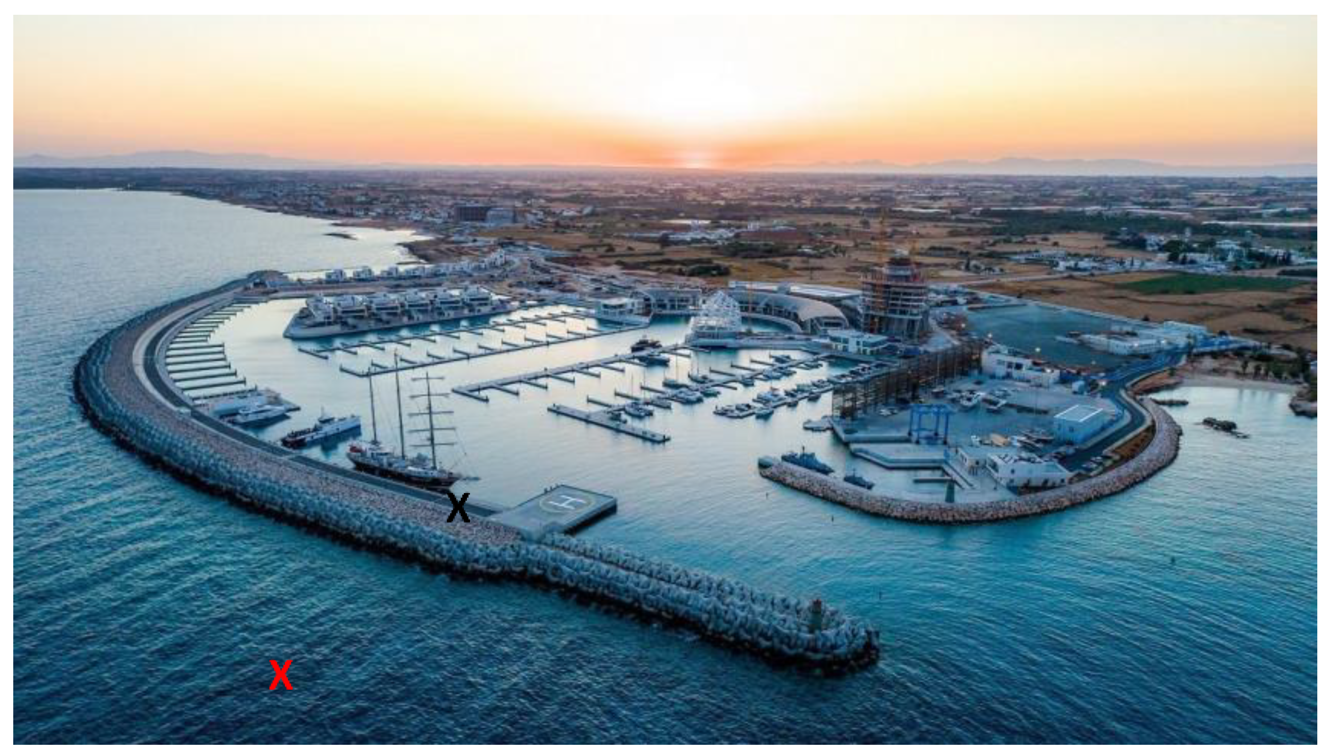
3.1. Site
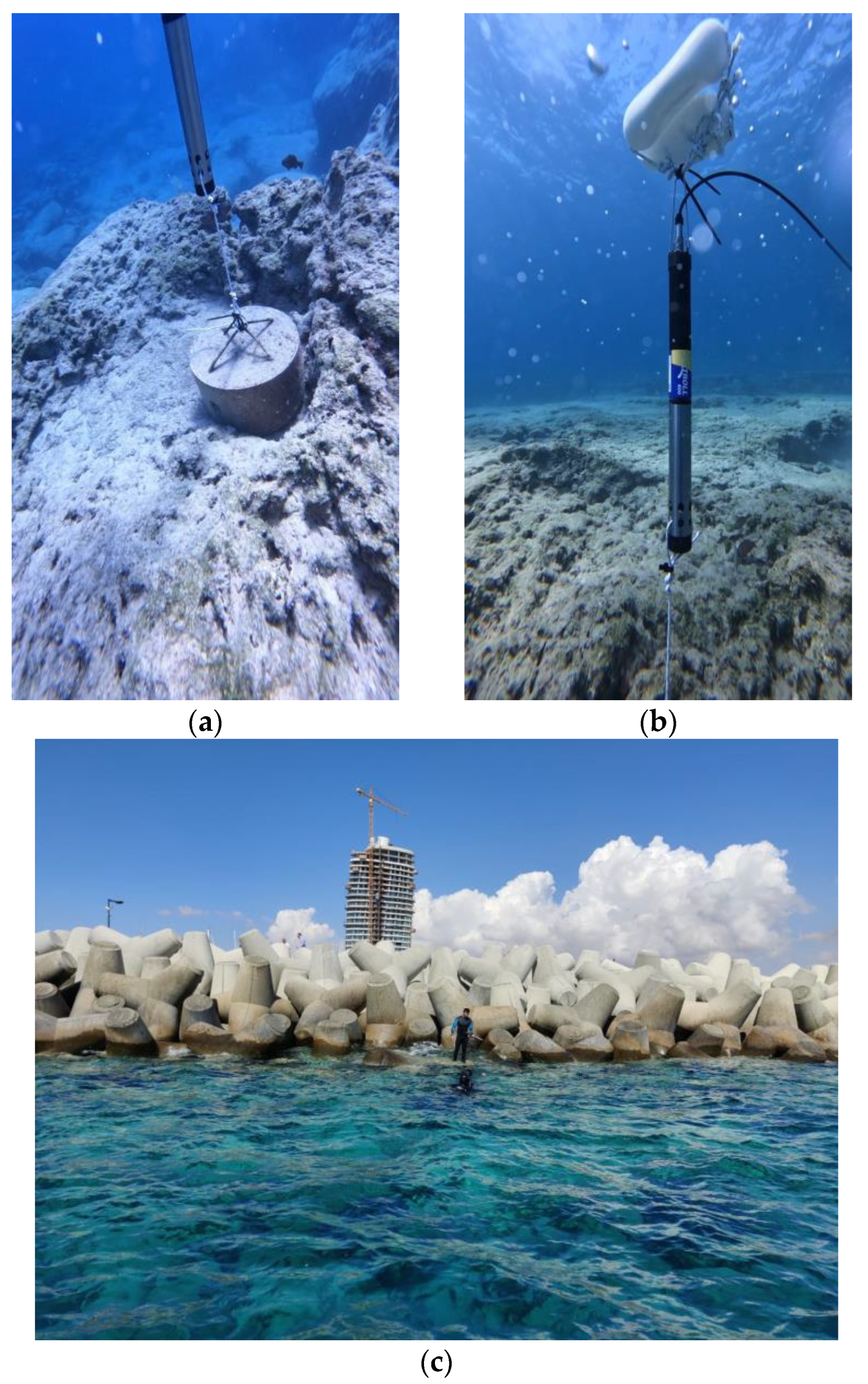
3.2. Installation and Connectivity
3.3. Deployment Considerations
3.4. Sampling Frequency
4. Data Quality Assessment and Processing
5. Lab Testing
6. In-Field Monitoring
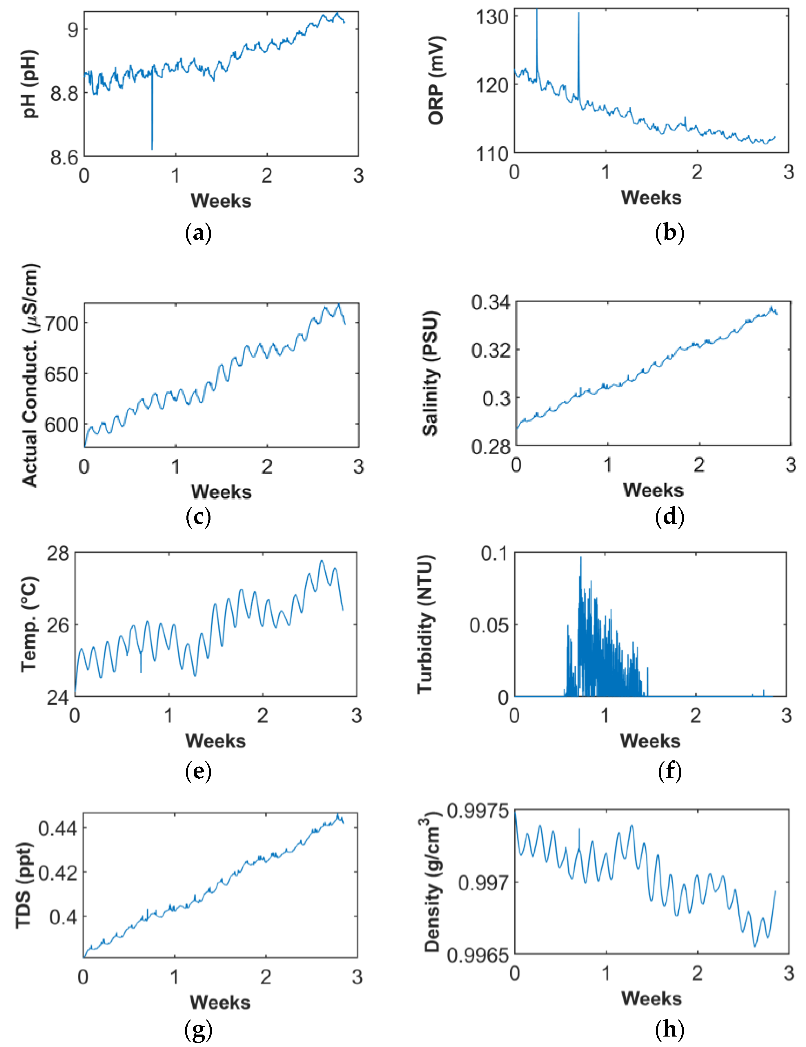
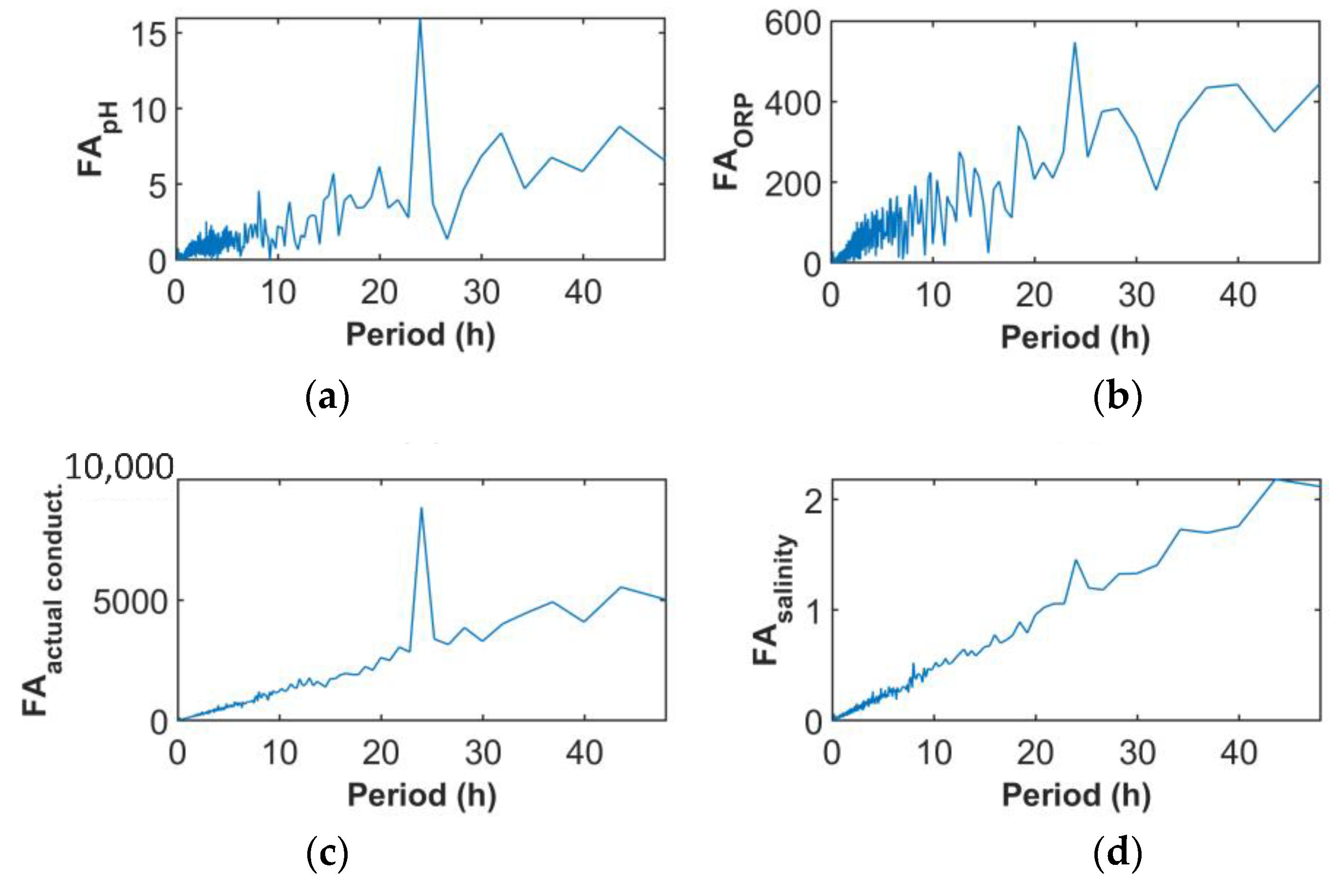
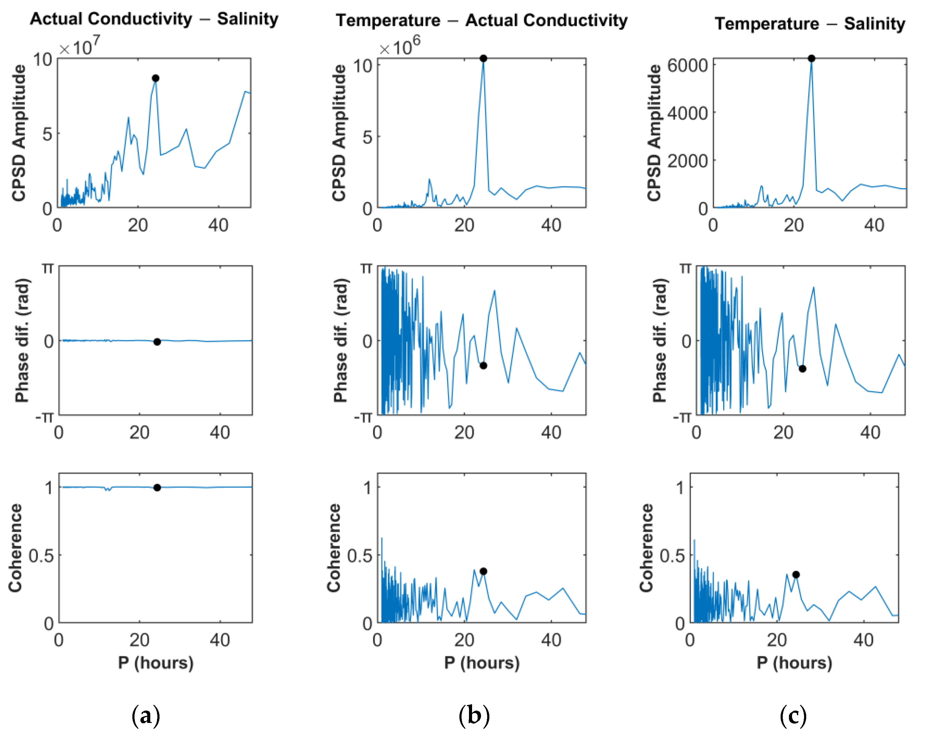
6.1. Time and Frequency Domain Data Interpretation
6.2. Data Noise Cancellation
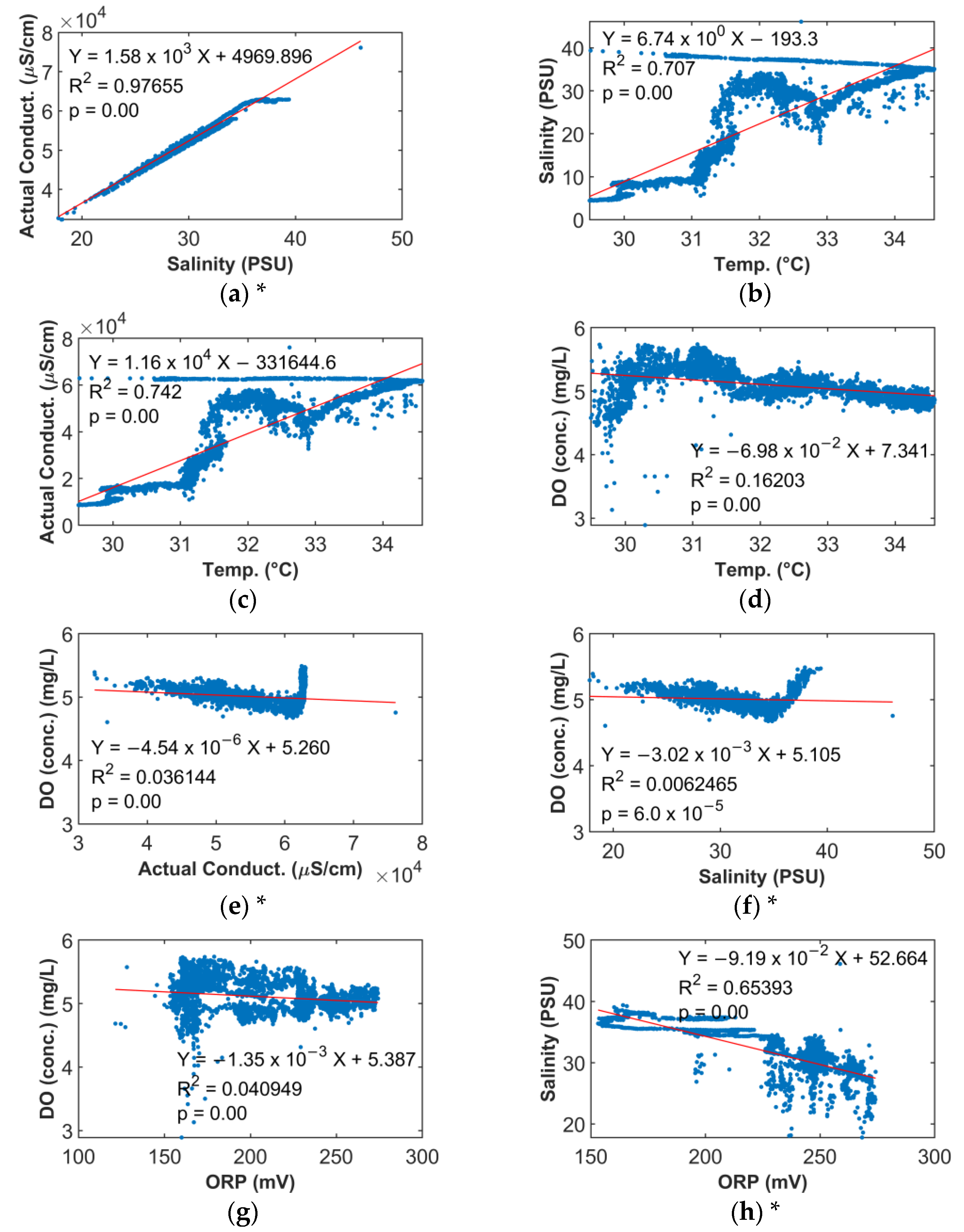
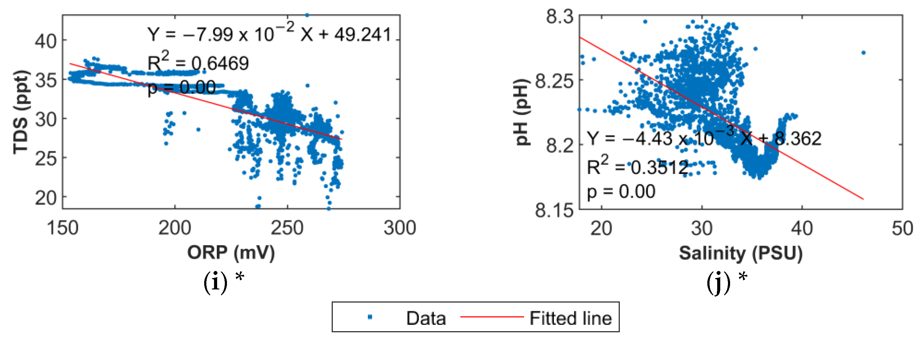
6.3. Water Quality Parameter Correlations
7. Discussion
7.1. Practical Outcomes from the Pilot System
7.2. Data Post-Processing
7.3. Seawater Quality
7.4. Time Variations and Correlations
8. Conclusions
Author Contributions
Funding
Data Availability Statement
Acknowledgments
Conflicts of Interest
Appendix A
| pH | ORP | DO (Sat.) | AC * | SC * | Salinity * | Temp. | Turbidity | TDS * | Density * | |
|---|---|---|---|---|---|---|---|---|---|---|
| pH | 1 | 1.43 × 10⁻⁶ | 1.37 × 10−103 | 0 | 2.90 × 10−240 | 1.48 × 10−243 | 3.36 × 10−183 | 1.10 × 10⁻⁹ | 2.89 × 10−240 | 9.92 × 10−176 |
| ORP | 1.43 × 10⁻⁶ | 1 | 0 | 0 | 0 | 0 | 0 | 3.84 × 10⁻¹ | 0 | 0 |
| DO (Sat.) | 1.37 × 10−103 | 0 | 1 | 3.99 × 10−307 | 0 | 0 | 0 | 3.76 × 10⁻¹ | 0 | 0 |
| AC * | 0 | 0 | 3.99 × 10−307 | 1 | 0 | 0 | 3.53 × 10−59 | 8.03 × 10⁻¹⁶ | 0 | 0 |
| SC * | 2.90 × 10−240 | 0 | 0 | 0 | 1 | 0 | 3.01 × 10⁻¹⁷ | 5.31 × 10⁻¹³ | 0 | 0 |
| Salinity * | 1.48 × 10−243 | 0 | 0 | 0 | 0 | 1 | 6.00 × 10⁻¹⁷ | 4.83 × 10⁻¹³ | 0 | 0 |
| Temp. | 3.36 × 10−183 | 0 | 0 | 3.53 × 10−59 | 3.01 × 10⁻¹⁷ | 6.00 × 10⁻¹⁷ | 1 | 6.92 × 10⁻¹¹ | 3.01 × 10⁻¹⁷ | 7.07 × 10⁻² ** |
| Turbidity | 1.10 × 10⁻⁹ | 3.84 × 10⁻¹ | 3.76 × 10⁻¹ | 8.03 × 10⁻¹⁶ | 5.31 × 10⁻¹³ | 4.83 × 10⁻¹³ | 6.92 × 10⁻¹¹ | 1 | 5.31 × 10⁻¹³ | 1.56 × 10⁻¹⁰ |
| TDSs * | 2.89 × 10−240 | 0 | 0 | 0 | 0 | 0 | 3.01 × 10⁻¹⁷ | 5.31 × 10⁻¹³ | 1 | 0 |
| Density * | 9.92 × 10−176 | 0 | 0 | 0 | 0 | 0 | 7.07 × 10⁻² ** | 1.56 × 10⁻¹⁰ | 0 | 1 |
References
- Pioch, S.; Kilfoyle, K.; Levrel, H.; Spieler, R. Green Marine Construction. Source J. Coast. Res. 2011, 61, 257–268. [Google Scholar] [CrossRef]
- El Gohary, R.; Hassan, N.A.A. Environmental Impact Assessment (EIA) of Marine Structures—A Case Study. KSCE J. Civ. Eng. 2012, 16, 689–698. [Google Scholar] [CrossRef]
- Lee, S.; Lee, E.; Yoo, H.S.; Lee, M.-J. Analysis of Trends in Marine Water Quality Using Environmental Impact Assessment Monitoring Data. Source: J. Coast. Res. 2020, 102, 39–46. [Google Scholar] [CrossRef]
- Yudhistira, M.H.; Karimah, I.D.; Maghfira, N.R. The Effect of Port Development on Coastal Water Quality: Evidence of Eutrophication States in Indonesia. Ecol. Econ. 2022, 196, 107415. [Google Scholar] [CrossRef]
- Jacob, C.; Pioch, S.; Thorin, S. The Effectiveness of the Mitigation Hierarchy in Environmental Impact Studies on Marine Ecosystems: A Case Study in France. Environ. Impact Assess. Rev. 2016, 60, 83–98. [Google Scholar] [CrossRef]
- Borja, Á.; Chust, G.; Rodríguez, J.G.; Bald, J.; Belzunce-Segarra, M.J.; Franco, J.; Garmendia, J.M.; Larreta, J.; Menchaca, I.; Muxika, I.; et al. ‘The Past Is the Future of the Present’: Learning from Long-Time Series of Marine Monitoring. Sci. Total Environ. 2016, 566, 698–711. [Google Scholar] [CrossRef]
- Tavakoly Sany, S.B.; Hashim, R.; Rezayi, M.; Salleh, A.; Safari, O. A Review of Strategies to Monitor Water and Sediment Quality for a Sustainability Assessment of Marine Environment. Environ. Sci. Pollut. Res. 2014, 21, 813–833. [Google Scholar] [CrossRef] [PubMed]
- Saengsupavanich, C.; Rif’atin, H.Q.; Magdalena, I.; Ariffin, E.H. A Systematic Review of Jetty-Induced Downdrift Coastal Erosion Management. Reg. Stud. Mar. Sci. 2024, 74, 103523. [Google Scholar] [CrossRef]
- Gómez, A.G.; Ondiviela, B.; Puente, A.; Juanes, J.A. Environmental Risk Assessment of Water Quality in Harbor Areas: A New Methodology Applied to European Ports. J. Environ. Manag. 2015, 155, 77–88. [Google Scholar] [CrossRef] [PubMed]
- Manjakkal, L.; Mitra, S.; Petillot, Y.R.; Shutler, J.; Scott, E.M.; Willander, M.; Dahiya, R. Connected Sensors, Innovative Sensor Deployment, and Intelligent Data Analysis for Online Water Quality Monitoring. IEEE Internet Things J. 2021, 8, 13805–13824. [Google Scholar] [CrossRef]
- Ramírez, A.; Morant, M.; Llorente, R. Underwater Optical Network for Remote Sensing Applications in Fluvial Environments. In Proceedings of the 21st International Conference on Transparent Optical Networks (ICTON), Angers, France, 9–13 July 2019; pp. 1–4. [Google Scholar]
- Karydis, M.; Kitsiou, D. Marine Water Quality Monitoring: A Review. Mar. Pollut. Bull. 2013, 77, 23–36. [Google Scholar] [CrossRef] [PubMed]
- Pasika, S.; Gandla, S.T. Smart Water Quality Monitoring System with Cost-Effective Using IoT. Heliyon 2020, 6, e04096. [Google Scholar] [CrossRef]
- Glasgow, H.B.; Burkholder, J.A.M.; Reed, R.E.; Lewitus, A.J.; Kleinman, J.E. Real-Time Remote Monitoring of Water Quality: A Review of Current Applications, and Advancements in Sensor, Telemetry, and Computing Technologies. J. Exp. Mar. Biol. Ecol. 2004, 300, 409–448. [Google Scholar] [CrossRef]
- Koričan, M.; Vladimir, N.; Stamatopoulou, E.A.; Ventikos, N.P.; Omanović, D. Early Warning System and Mobile App for Marine Pollution Prevention. In Proceedings of the International Conference on Electrical, Computer, Communications and Mechatronics Engineering, ICECCME 2022, Maldives, Maldives, 16–18 November 2022; Institute of Electrical and Electronics Engineers Inc.: New York, NY, USA, 2022. [Google Scholar]
- Ahmed, U.; Mumtaz, R.; Anwar, H.; Mumtaz, S.; Qamar, A.M. Water Quality Monitoring: From Conventional to Emerging Technologies. Water Sci. Technol. Water Supply 2020, 20, 28–45. [Google Scholar] [CrossRef]
- Bennett, K.; Ilvonen, A.; Bennett, A. Extended Deployment of an Automated Coastal Environment Monitoring System. In Proceedings of the OCEANS 2022, Hampton Roads, VA, USA, 17–20 October 2022; Institute of Electrical and Electronics Engineers Inc.: New York, NY, USA, 2022; pp. 1–9. [Google Scholar]
- Snow, C.; Zeng, J.; Nonas-Hunter, L.; Diggins, D.; Bennett, K.; Bennett, A. Design of a Cable-Mounted Robot for near Shore Monitoring. In Proceedings of the Global Oceans 2020: Singapore—U.S. Gulf Coast, Biloxi, MS, USA, 5–30 October 2020; Institute of Electrical and Electronics Engineers Inc.: New York, NY, USA, 2020. [Google Scholar]
- Bennett, K.R.; Zeng, J.; Diggins, D.; Nonas-Hunter, L.; Snow, C.; Bennett, A.A. The Development and Implementation of an Automated Coastal Environment Monitoring System. In Proceedings of the 2020 Global Oceans 2020: Singapore—U.S. Gulf Coast, Biloxi, MS, USA, 5–30 October 2020; Institute of Electrical and Electronics Engineers Inc.: New York, NY, USA, 2020. [Google Scholar]
- Jiang, J.; Tang, S.; Han, D.; Fu, G.; Solomatine, D.; Zheng, Y. A Comprehensive Review on the Design and Optimization of Surface Water Quality Monitoring Networks. Environ. Model. Softw. 2020, 132, 104792. [Google Scholar] [CrossRef]
- Meyers, D.; Zheng, Q.; Duarte, F.; Ratti, C.; Hemond, H.F.; van der Blom, M.; van der Helm, A.W.C.; Whittle, A.J. Initial Deployment of a Mobile Sensing System for Water Quality in Urban Canals. Water 2022, 14, 2834. [Google Scholar] [CrossRef]
- Danovaro, R.; Carugati, L.; Berzano, M.; Cahill, A.E.; Carvalho, S.; Chenuil, A.; Corinaldesi, C.; Cristina, S.; David, R.; Dell’Anno, A.; et al. Implementing and Innovating Marine Monitoring Approaches for Assessing Marine Environmental Status. Front. Mar. Sci. 2016, 3, 213. [Google Scholar] [CrossRef]
- Jahanbakht, M.; Xiang, W.; Hanzo, L.; Azghadi, M.R. Internet of Underwater Things and Big Marine Data Analytics—A Comprehensive Survey. IEEE Commun. Surv. Tutor. 2021, 23, 904–956. [Google Scholar] [CrossRef]
- Lakshmikantha, V.; Hiriyannagowda, A.; Manjunath, A.; Patted, A.; Basavaiah, J.; Anthony, A.A. IoT Based Smart Water Quality Monitoring System. Glob. Transit. Proc. 2021, 2, 181–186. [Google Scholar] [CrossRef]
- Zhang, X.; Zhang, Y.; Zhang, Q.; Liu, P.; Guo, R.; Jin, S.; Liu, J.; Chen, L.; Ma, Z.; Ying, L. Evaluation and Analysis of Water Quality of Marine Aquaculture Area. Int. J. Environ. Res. Public Health 2020, 17, 1446. [Google Scholar] [CrossRef]
- Tsai, K.L.; Chen, L.W.; Yang, L.J.; Shiu, H.; Chen, H.W. IoT Based Smart Aquaculture System with Automatic Aerating and Water Quality Monitoring. J. Internet Technol. 2022, 23, 177–184. [Google Scholar] [CrossRef]
- Duque, C.; Knee, K.L.; Russoniello, C.J.; Sherif, M.; Abu Risha, U.A.; Sturchio, N.C.; Michael, H.A. Hydrogeological Processes and near Shore Spatial Variability of Radium and Radon Isotopes for the Characterization of Submarine Groundwater Discharge. J. Hydrol. 2019, 579, 124192. [Google Scholar] [CrossRef]
- Yu, X.; Liu, J.; Chen, X.; Yu, H.; Du, J. Fresh and Saline Groundwater Nutrient Inputs and Their Impacts on the Nutrient Budgets in a Human-Effected Bay. Mar. Pollut. Bull. 2024, 199, 116026. [Google Scholar] [CrossRef]
- Onoufriou, T.; Michailides, C.; Christodoulides, P. Digitisation and Proactive Management of Coastal and Offshore Infrastructure and Environment. In Proceedings of the 2nd International Conference on Design and Management of Port, Coastal and Offshore works DMPCO 2023, Thessaloniki, Greece, 24 May 2023; pp. 82–86. [Google Scholar]
- In-Situ Europe Ltd. Aqua TROLL 600 Multiparameter Sonde.; In-Situ Europe Ltd.: Worcestershire, UK, 2024. [Google Scholar]
- Baird, R.B.; Eaton, A.D.; Rice, E.W. Standard Methods for the Examination of Water and Wastewater, 23rd ed.; Americal Public Health Association: Washington, DC, USA, 2017. [Google Scholar]
- Chester, R.; Jickells, T. Marine Geochemistry, 3rd ed.; Wiley-Blackwell: Hoboken, NJ, USA, 2012; ISBN 9781118349076. [Google Scholar]
- Verma, A.K.; Singh, T.N. Prediction of Water Quality from Simple Field Parameters. Environ. Earth Sci. 2013, 69, 821–829. [Google Scholar] [CrossRef]
- Lorenzoni, L.; Telszewski, M.; Benway, H.; Palacz, A. A User’s Guide for Selected Autonomous Biogeochemical Sensors; An Outcome from the 1st International IOCCP Sensors Summer Course—Instrumenting Our Oceans for Better Observations; IOCCP: Sopot, Poland, 2015. [Google Scholar]
- Håkanson, L.; Blenckner, T. A Review on Operational Bioindicators for Sustainable Coastal Management-Criteria, Motives and Relationships. Ocean Coast. Manag. 2008, 51, 43–72. [Google Scholar] [CrossRef]
- Roberge, P.R. Handbook of Corrosion Engineering, 3rd ed.; McGraw-Hill: New York, NY, USA, 2019. [Google Scholar]
- Lewis, E.L.; Perkin, R.G. Salinity: Its Definition and Calculation. J. Geophys. Res. 1978, 83, 466–478. [Google Scholar] [CrossRef]
- Ushkov, A.N.; Strelkov, N.O.; Krutskikh, V.V.; Chernikov, A.I. Industrial Internet of Things Platform for Water Resource Monitoring. In Proceedings of the International Russian Smart Industry Conference, Sochi, Russia, 27–31 March 2023; Institute of Electrical and Electronics Engineers Inc.: New York, NY, USA, 2023; pp. 593–599. [Google Scholar]
- Vilmin, L.; Flipo, N.; Escoffier, N.; Groleau, A. Estimation of the Water Quality of a Large Urbanized River as Defined by the European WFD: What Is the Optimal Sampling Frequency? Environ. Sci. Pollut. Res. 2018, 25, 23485–23501. [Google Scholar] [CrossRef]
- Prasad, R.; Anuprakash, M.V. Pollution Due to Oil Spills in Marine Environment And Control Measures. IOSR J. Environ. Sci. Toxicol. Food Technol. 2016, 10, 1–8. [Google Scholar] [CrossRef]
- Koronides, M.; Kontoe, S.; Zdravković, L.; Vratsikidis, A.; Pitilakis, D. Numerical Simulation of SSI Free and Forced Vibration Experiments on Real Scale Structures of Different Stiffness. Soil Dyn. Earthq. Eng. 2023, 175, 108232. [Google Scholar] [CrossRef]
- Koronides, M.; Kontoe, S.; Zdravković, L.; Vratsikidis, A.; Pitilakis, D.; Anastasiadis, A.; Potts, D.M. Numerical Simulation of Real-Scale Vibration Experiments of a Steel Frame Structure on a Shallow Foundation. In Geotechnical, Geological and Earthquake Engineering, Proceedings of the 4th International Conference on Performance-Based Design in Earthquake Engineering, Beijing, China, 15–17 July 2022; Wang, L., Zhang, J.-M., Wang, R., Eds.; Springer International Publishing: Cham, Switzerland, 2022; pp. 1119–1127. [Google Scholar]
- Rodriguez-Espinosa, P.F.; Fonseca-Campos, J.; Ochoa-Guerrero, K.M.; Hernandez-Ramirez, A.G.; Tabla-Hernandez, J.; Martínez-Tavera, E.; Lopez-Martínez, E.; Jonathan, M.P. Identifying Pollution Dynamics Using Discrete Fourier Transform: From an Urban-Rural River, Central Mexico. J. Environ. Manag. 2023, 344, 118173. [Google Scholar] [CrossRef] [PubMed]
- Kim, S.; Stewart, J.P. Kinematic Soil-Structure Interaction from Strong Motion Recordings. J. Geotech. Geoenviron. Eng. 2003, 129, 323–335. [Google Scholar] [CrossRef]
- State General Laboratory of the Republic of Cyprus. Available online: https://www.moh.gov.cy/Moh/SGL/sgl.nsf/home_en/home_en?opendocument (accessed on 1 August 2024).
- European Union. Directive (EU) 2020/2184 On the Quality of Water Intended for Human Consumption. Off. J. Eur. Union 2020, L 435/1, 1–62. [Google Scholar]
- Hadjisolomou, E.; Antoniadis, K.; Vasiliades, L.; Rousou, M.; Thasitis, I.; Abualhaija, R.; Herodotou, H.; Michaelides, M.; Kyriakides, I. Predicting Coastal Dissolved Oxygen Values with the Use of Artificial Neural Networks: A Case Study for Cyprus. In Proceedings of the IOP Conference Series: Earth and Environmental Science, Depok, Indonesia, 27–28 August 2022; Institute of Physics: Bristol, UK, 2022; Volume 1123. [Google Scholar]
- Hadjisolomou, E.; Rousou, M.; Antoniadis, K.; Vasiliades, L.; Kyriakides, I.; Herodotou, H.; Michaelides, M. Data-Driven Models for Evaluating Coastal Eutrophication: A Case Study for Cyprus. Water 2023, 15, 4097. [Google Scholar] [CrossRef]
- Li, Z.; Sheng, Y.; Yang, J.; Burton, E.D. Phosphorus Release from Coastal Sediments: Impacts of the Oxidation-Reduction Potential and Sulfide. Mar. Pollut. Bull. 2016, 113, 176–181. [Google Scholar] [CrossRef] [PubMed]
- Liu, X.; Wang, J.; Zhang, D.; Li, Y. Grey Relational Analysis on the Relation between Marine Environmental Factors and Oxidation-Reduction Potential. Chin. J. Oceanol. Limnol. 2009, 27, 583–586. [Google Scholar] [CrossRef]
- Zheng, Z.; Fu, Y.; Liu, K.; Xiao, R.; Wang, X.; Shi, H. Three-Stage Vertical Distribution of Seawater Conductivity. Sci. Rep. 2018, 8, 9916. [Google Scholar] [CrossRef] [PubMed]
- Macdonald, R.K.; Ridd, P.V.; Whinney, J.C.; Larcombe, P.; Neil, D.T. Towards Environmental Management of Water Turbidity within Open Coastal Waters of the Great Barrier Reef. Mar. Pollut. Bull. 2013, 74, 82–94. [Google Scholar] [CrossRef] [PubMed]
- Rusydi, A.F. Correlation between Conductivity and Total Dissolved Solid in Various Type of Water: A Review. In Proceedings of the IOP Conference Series: Earth and Environmental Science, Banda Aceh, Indonesia, 26–27 September 2018; Institute of Physics Publishing: Bristol, UK, 2018; Volume 118. [Google Scholar]
- Rahman, M.H.; Pandit, D.; Begum, N.; Sikder, M.N.A.; Preety, Z.N.; Roy, T.K. Fluctuations of Physicochemical Parameters in the Waters of the Chattogram Coastal Area, Bangladesh. Mar. Sci. Technol. Bull. 2023, 12, 530–539. [Google Scholar] [CrossRef]
- Koronides, M. Numerical and Field Investigation of Dynamic Soil Structure Interaction at Full-Scale; Imperial College London: London, UK, 2023. [Google Scholar]


| Parameter | Mean | Min | Max | Parametric Value Aligned with EU Directive | Reference Values |
|---|---|---|---|---|---|
| pH (pH) | 8.90 | 8.62 | 9.50 | ≥6.5 and ≤9.5 | 8.5–8.7 |
| DO Conc. (mg/L) | 6.16 | 5.67 | 7.16 | - | 7.8–8.2 * |
| Specific Cond. (µS/cm) | 633.15 | 586.13 | 687.06 | ≤2500 | 760–900 |
| TDS (ppt) | 0.41 | 0.38 | 0.45 | - | 0.3–0.4 |
| Turbidity (NTU) | 0.0044 | 0 | 1.3 | Acceptable to consumers and no abnormal change | 0.3 * |
| Measured | Reference Values | ||||
|---|---|---|---|---|---|
| Parameter | Mean ± SD | Min | Max | For the Coastal Area of Cyprus [47,48] ** Mean ± SD (min–max) | For Coastal Waters in General |
| pH (pH) | 8.25 ± 0.05 | 8.17 | 8.36 | 7.9 ± 0.5 (6.6–8.8) | 7.9–9.0 [26] |
| ORP (mV) | 210.33 ± 36.46 | 128.13 | 274.22 | - | 100–500 [49,50] |
| DO conc. (mg/L) | 5.13 ± 0.22 | 2.89 | 5.74 | 7.8 ± 0.4 (1.6–8.6) | 1.5–8.5 [50] but typically 7–8 |
| DO sat. (%) | 80.40 ± 4.49 | 40.24 | 92.54 | - | - |
| Actual Cond. (mS/cm) * | 41.74 ± 17.98 | 10.92 | 76.11 | 56.3 ± 4.8 (0.8–67.2) | 30–60 [51] |
| Specific Cond. (mS/cm) * | 36.42 ± 15.26 | 9.77 | 66.44 | - | - |
| Salinity (PSU) * | 23.78 ± 10.75 | 5.58 | 46.11 | 37.7 ± 2.9 (0.86–44.1) | 31–36 [28] |
| Temperature (°C) | 32.19 ± 1.34 | 29.50 | 34.59 | 16 (winter), 26 (summer) (15–36) *** | - |
| Turbidity (NTU) | 38.54 ± 223.21 | 0.00 | 4410.20 | - | 0.1–100 [52] |
| TDS (ppt) * | 23.67 ± 9.92 | 6.35 | 43.19 | - | 19–40 [53,54] |
| Density (g/cm3) * | 1.01 ± 0.008 | 1.00 | 1.03 | - | 1.0 |
| pH | ORP | DO (Sat.) | AC * | SC * | Salinity * | Temp. | Turbidity | TDS * | Density * | |
|---|---|---|---|---|---|---|---|---|---|---|
| P10 | 8.188 | 161.04 | 69.71 | 47,120.56 | 41,153.48 | 26.84 | 30.02 | 0.00 | 26.75 | 1.015 |
| P20 | 8.201 | 163.89 | 74.68 | 50,121.00 | 43,793.11 | 28.77 | 30.54 | 0.04 | 28.47 | 1.016 |
| P50 | 8.259 | 205.05 | 80.72 | 55,547.79 | 48,202.94 | 32.04 | 31.68 | 7.39 | 31.33 | 1.018 |
| P80 | 8.314 | 246.49 | 83.34 | 61,997.15 | 52,618.17 | 35.37 | 33.60 | 25.39 | 34.20 | 1.020 |
| pH | ORP | DO (Sat.) | AC * | SC * | Salinity * | Temp. | Turbidity | TDS * | Density * | |
|---|---|---|---|---|---|---|---|---|---|---|
| pH | 1 | 0.070 | 0.307 | −0.664 | −0.589 | −0.593 | −0.403 | 0.089 | −0.589 | −0.517 |
| ORP | 0.070 | 1 | 0.590 | −0.796 | −0.804 | −0.809 | 0.583 | −0.013 | −0.804 | −0.802 |
| DO (Sat.) | 0.307 | 0.590 | 1 | 0.649 | 0.687 | 0.692 | 0.605 | −0.013 | 0.687 | 0.707 |
| AC * | −0.664 | −0.796 | 0.649 | 1.000 | 0.999 | 0.999 | 0.869 | −0.158 | 0.989 | 0.955 |
| SC * | −0.589 | −0.804 | 0.687 | 0.999 | 1.000 | 1.000 | 0.854 | −0.142 | 1.000 | 0.986 |
| Salinity * | −0.593 | −0.809 | 0.692 | 0.999 | 1.000 | 1.000 | 0.850 | −0.142 | 1.000 | 0.986 |
| Temp. | −0.403 | 0.583 | 0.605 | 0.869 | 0.854 | 0.850 | 1.000 | −0.095 | 0.854 | 0.036 ** |
| Turbidity | 0.089 | −0.013 | −0.013 | −0.158 | −0.142 | −0.142 | −0.095 | 1 | −0.142 | −0.126 |
| TDSs * | −0.589 | −0.804 | 0.687 | 0.989 | 1.000 | 1.000 | 0.854 | −0.142 | 1 | 0.986 |
| Density * | −0.517 | −0.802 | 0.707 | 0.955 | 0.986 | 0.986 | 0.036 ** | −0.126 | 0.986 | 1 |
Disclaimer/Publisher’s Note: The statements, opinions and data contained in all publications are solely those of the individual author(s) and contributor(s) and not of MDPI and/or the editor(s). MDPI and/or the editor(s) disclaim responsibility for any injury to people or property resulting from any ideas, methods, instructions or products referred to in the content. |
© 2024 by the authors. Licensee MDPI, Basel, Switzerland. This article is an open access article distributed under the terms and conditions of the Creative Commons Attribution (CC BY) license (https://creativecommons.org/licenses/by/4.0/).
Share and Cite
Koronides, M.; Stylianidis, P.; Michailides, C.; Onoufriou, T. Real-Time Monitoring of Seawater Quality Parameters in Ayia Napa, Cyprus. J. Mar. Sci. Eng. 2024, 12, 1731. https://doi.org/10.3390/jmse12101731
Koronides M, Stylianidis P, Michailides C, Onoufriou T. Real-Time Monitoring of Seawater Quality Parameters in Ayia Napa, Cyprus. Journal of Marine Science and Engineering. 2024; 12(10):1731. https://doi.org/10.3390/jmse12101731
Chicago/Turabian StyleKoronides, Marios, Panagiotis Stylianidis, Constantine Michailides, and Toula Onoufriou. 2024. "Real-Time Monitoring of Seawater Quality Parameters in Ayia Napa, Cyprus" Journal of Marine Science and Engineering 12, no. 10: 1731. https://doi.org/10.3390/jmse12101731