Identification of Fish Hunger Degree with Deformable Attention Transformer

Abstract

Feeding is a critical process in aquaculture, as it has a direct impact on the quantity and quality of fish. With advances in convolutional neural network (CNN) and vision transformer (ViT), intelligent feeding has been widely adopted in aquaculture, as the real-time monitoring of fish behavior can lead to better feeding decisions. However, existing models still have the problem of insufficient accuracy in the fish behavior-recognition task. In this study, the largemouth bass (Micropterus salmoides) was selected as the research subject, and three categories (weakly, moderately, and strongly hungry) were defined. We applied the deformable attention to the vision transformer (DeformAtt-ViT) to identify the fish hunger degree. The deformable attention module was extremely powerful in feature extraction because it improved the fixed geometric structure of the receptive fields with data-dependent sparse attention, thereby guiding the model to focus on more important regions. In the experiment, the proposed DeformAtt-ViT was compared with the state-of-the-art transformers. Among them, DeformAtt-ViT achieved optimal performance in terms of accuracy, F1-score, recall, and precision at 95.50%, 94.13%, 95.87%, and 92.45%, respectively. Moreover, a comparative evaluation between DeformAtt-ViT and CNNs was conducted, and DeformAtt-ViT still dominated the others. We further visualized the important pixels that contributed the most to the classification result, enabling the interpretability of the model. As a prerequisite for determining the feed time, the proposed DeformAtt-ViT could identify the aggregation level of the fish and then trigger the feeding machine to be turned on. Also, the feeding machine will stop working when the aggregation disappears. Conclusively, this study was of great significance, as it explored the field of intelligent feeding in aquaculture, enabling precise feeding at a proper time.

1. Introduction

Aquatic products have been increasingly recognized for their key role in providing food and nutrition because they can contribute about 17 percent of animal protein, accounting for over 50 percent in many developing countries in Asia and Africa [1]. In 2020, global aquaculture production reached a record of 122.6 million tons, and the world’s consumption of aquaculture production is estimated to continuously rise. With the development of various techniques like the Internet of Things (IoT) and artificial intelligence (AI), traditional labor-intensive aquaculture methods have transformed into smart automated systems [2]. For instance, as a key practice in aquaculture, the traditional feeding method requires a human to determine the feeding frequency and quantity, leading to an increase in the feeding cost and bait waste. Research on intelligent feeding systems in aquaculture has been gaining momentum in recent years due to the potential benefits they offer in terms of optimizing feeding practices, improving efficiency, and reducing environmental impact [3,4,5]. In particular, the feeding system usually first recognizes the fish’s behavior, thereby guiding the feeding practice according to the degree of hunger [6].

It is estimated that feeding expenses account for up to 50% of the total production cost [7]. On the one hand, over-feeding may reduce production efficiency and the excess amount of baits would cause serious issues, such as water contamination and disease. On the other hand, underfeeding would slow the growth rate of fish and even lead to aggressive competition for food [8]. It is also noted that many factors, such as water turbidity, temperature, dissolved oxygen content, pH, nitrogen, and ammonia concentration, can also have an impact on the fish’s appetite [9,10,11,12]. Therefore, monitoring the fish’s behavior and identifying their hunger degree is extremely helpful for determining the feeding time and the quantity of baits to be released.

Recent advances in computer vision have made it possible to analyze fish behavior quickly and non-destructively. In general, the computer-vision technique is a branch of AI, and its goal is to replace human vision with digital cameras (e.g., RGB, RGB-D, and hyperspectral cameras) for observation. After obtaining the images, deep learning (DL) is a preferable approach for recognizing fish behavior. The merit of the DL-based model includes automatic feature extraction, and it can learn semantic information from a given image [13]. Various researchers have reported several successful neural networks in the task of fish behavior recognition. Iqbal et al. [14] proposed an effective end-to-end convolutional neural network (CNN) that can classify fish behavior into two categories: normal and hungry. By integrating three fully connected layers and max pooling operations, the accuracy of the network was improved by 10%. Zhu et al. [15] identified the feeding status of fish by applying a lightweight neural network, MobileNetV3-Small. They classified the degree of appetite of bass into four grades, namely strong, medium, weak, and none. To make the classification more practical, strong and medium appetites were divided into hungry categories, and weak and no appetites were divided into non-hungry categories. Zhou et al. [16] proposed a feeding-intensity assessment system based on the LeNet5 framework, which divided the feeding intensity into four levels, namely, none, weak, medium, and strong.

The traditional convolutional kernels used in the previous approach have fixed sampling positions and pooling layers, which limit the model’s ability to adapt to the complex spatial structure in the image. In contrast, the deformable convolutional neural network (DCNN) introduces deformable convolutional sampling positions that can be adjusted in size and shape based on the complex spatial context of the image. Experimental results have demonstrated that DCNN can achieve better classification performance when compared with typical CNN classification methods like VGG [17] and ResNet [18]. Chen et al. [19] proposed a novel DCNN framework to exploit classification for imbalanced water inflow in rock tunnel faces, and the experimental results showed that it outperformed well-known models in terms of both classification map quality and classification accuracy.

The transformer model [20] was originally developed for natural language processing. In recent years, a variant of this model called vision transformer has shown remarkable performance in computer-vision tasks [21]. As a result, researchers have started to use vision transformer models for fish-feeding behavior recognition and detection. Li et al. [22] proposed a transformer-based multiple fish tracking model to solve the problem of instance loss of fish targets in aquaculture ponds. Zeng et al. [23] proposed a recognition model for fish-feeding behavior that used a sliding window to convert acoustic signals into spectral features, and they used the hierarchical structure of the Swin transformer model to combine shift patch tokenization, local self-attention, and other modules, finally completing the classification task of fish-feeding behavior. Xia et al. [24] introduced a novel deformable attention-based vision transformer, called DAT, which combined the strengths of DCNN and the Swin transformer. DAT has demonstrated its effectiveness by achieving outstanding performance on widely used public datasets, such as ImageNet and COCO.

However, the application of DAT in some specific domains, such as fish behavior recognition, is still limited. Most of the researchers have focused on applying CNN to classify fish behavior, and they did not compare with the vision transformer, nor did they use deformable attention. But recent advances in vision transformers (ViTs) have shown excellent results compared with CNNs [25]. Therefore, further research is needed to apply ViTs in the aquaculture domain. Finally, deep-learning models are often considered a “black box”, meaning that the decision-making mechanism of these models is not transparent. It is noted that the model transparency allows users to have confidence during decision-making. In this study, the largemouth bass (Micropterus salmoides) was chosen as the research subject, and the main contributions of this paper can be summarized as follows.

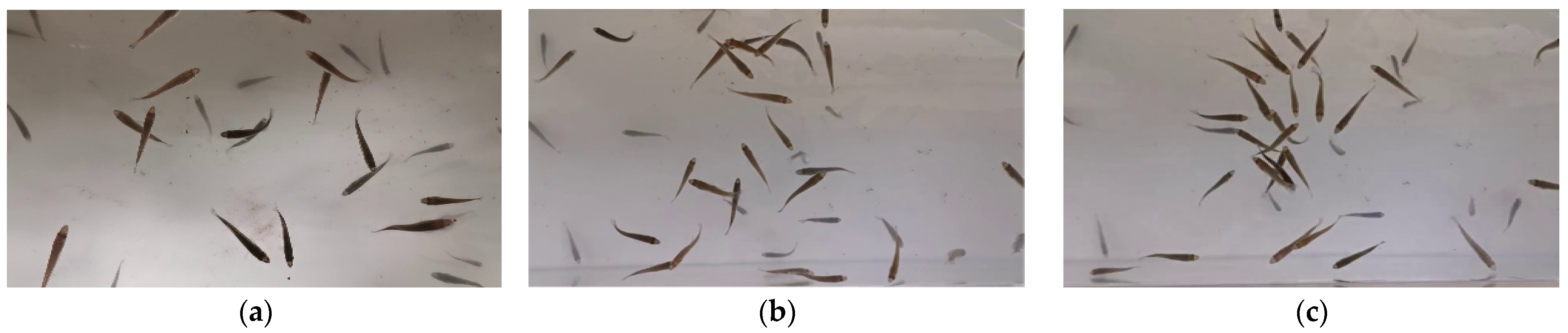
• We constructed a dataset of fish hunger degrees. Three degrees, including weakly, moderately, and strongly hungry, were defined based on the aggregation levels of fish. The established dataset was then used to train and validate the proposed detection model;
• We proposed the DeformAtt-ViT model by integrating the transformer architecture and the deformable attention mechanism to classify the fish hunger degree. The use of the deformable attention mechanism enabled DeformAtt-ViT to adaptively concentrate on the spatial features that were important to generate the final predictions. The comparative experiment verified the effectiveness of DeformAtt-Vit through the evaluation criteria, including accuracy, precision, F1-score, etc. By accurately classifying the hunger level, we can provide guidance on the appropriate time and bait amount to feed the fish;
• We utilized the Grad-CAM method to provide insights into the decision-making process for both CNNs and ViTs. This approach allowed us to visualize the pixels that contributed the most to the model’s predictions in a given image.

2. Materials and Methods

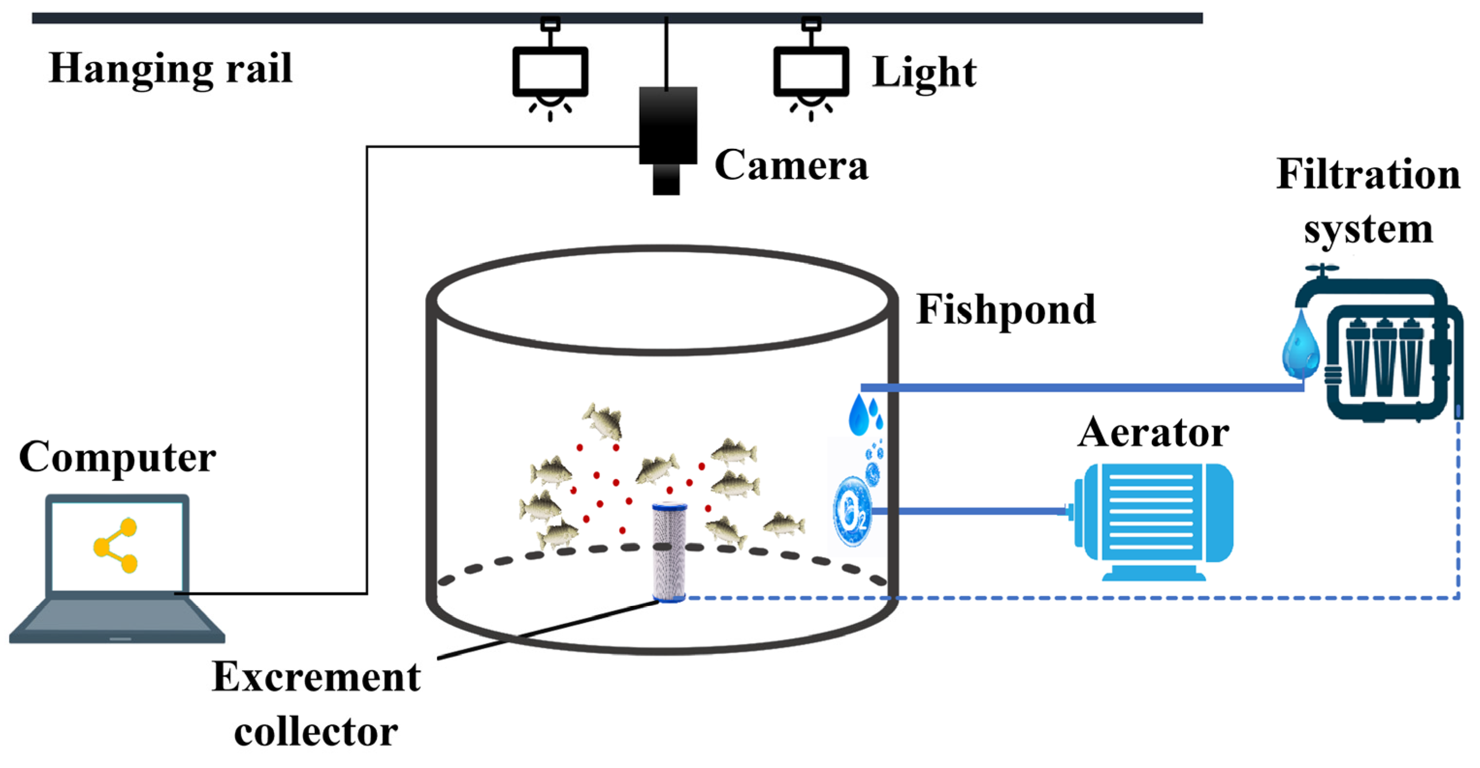
2.1. Fish Samples and Dataset Creation

In this experiment, largemouth basses (4 to 6 cm in length) were used for data collection in a fish tank with a diameter of 1.4 m and a height of 0.5 m. We divided the same batch of 200 basses into two groups. One group was fed manually at 10 am each day regularly. The other group was subjected to controlled feeding stress, with feeding conducted every five days (also at 10 am) to facilitate data collection under hunger conditions. These bass had been domesticated to eat bait and acclimated to the environment. The water temperature was set to 18 °C (maintained by a heater) and the pH value was maintained between 7 and 7.5, which was the most suitable growth temperature for bass [26]. Oxygen was sufficiently provided with an aeration pump. We used two light sources to ensure the illumination during data collection. Since the experiment was carried out indoors, the light sources were also used to simulate day and night. To be exact, the lights were turned on from 6 am to 8 pm and turned off during the rest of the time. The luminous intensity of the light source was around 1800 lx. Meanwhile, the largemouth bass received one feeding a day for 2 weeks before data collection. The water treatment system was used to treat fish excrement and tail water in the fish tank. A camera (Canon EOS 70D) was set up above the fish tank, and the schematic diagram is shown in Figure 1. We used this camera to capture videos of largemouth bass feeding at different hunger intensities, and the original video data was acquired at around 8 am and lasted for 4 h. Then, the downsampling operation was performed over these videos to obtain image frames by extracting representative images from them to be our dataset images. The acquired images were eventually transferred to a computer for further processing. The original resolution of the acquired image was 1280 × 720, and we resized it to 224 × 224 before inputting it to the model.

A total of 1600 images were obtained. These images were then categorized into 3 states: weakly, moderately, and strongly hungry. Additionally, a combination of the relevant literature and expertise from aquaculture experts was used to classify the hunger state of the images during the feeding period of the fish school. In total, the images were categorized into 757 images depicting a weakly hungry degree, 154 images representing a moderately hungry level, and 689 images illustrating a state of strong hunger. The original datasets of these three states are illustrated in Figure 2.

For the category of weakly hungry, the largemouth basses were fed regularly, and the images were taken when they did not respond to food. To induce a state of strong hunger, the largemouth basses were intentionally deprived of bait for a period of 5 days. This was done to create an environment of starvation and accurately capture the hunger degree of the fish. It was noted that the largemouth basses would move around in search of food, gather within a certain area, and float to the water surface more frequently when strongly hungry. As the largemouth basses consumed a certain amount of feed, the degree level of hunger decreased. If feeding was continued at this point, their feeding behavior would slow down, and the intensity of bass gathering and competing for food would decrease. This degree was considered moderately hungry, indicating that the fish have consumed enough to alleviate their initial hunger but are still in need of additional nourishment.

2.2. Network Architecture of DeformAtt-ViT

DeformAtt-ViT is a universal backbone network model with deformable attention. In terms of network architecture, DeformAtt-ViT has replaced the previous multi-head self-attention (MHSA) and combined it with a multi-layer perceptron (MLP) to construct the deformable vision transformer block. To build a hierarchical feature pyramid, the backbone consists of four stages where the stride gradually increases. Between two consecutive stages, a non-overlapping 2 × 2 convolution with a stride of 2 is applied to perform the downsampling operation over the feature map, thereby reducing the spatial dimension by half and doubling the feature size.

The backbone architecture primarily consists of four stages. Prior to Stage 1, the model processes the input fish images with a shape of H × W × 3 using non-overlapping 4 × 4 convolutions with a stride of 4 to obtain embeddings. These embeddings are then normalized to obtain patch embeddings of size (H/4) × (W/4) × C. In the first two stages, the feature maps have a rather large spatial size, leading to the fact that the computational workload, i.e., the dot product and bilinear interpolation, would be extremely heavy. Therefore, we adopted the shift window attention of the Swin transformer during early feature learning [27]. In the latter two stages (i.e., Stages 3 and 4), as the keys and values decrease, the deformable attention module is applied to obtain the global relationships between local tokens. The overall architecture of DeformAtt-ViT is shown in Figure 3. Successive local attention and deformable attention blocks are introduced in the latter two stages. The purpose of local attention is to process the input feature maps and obtain locally aggregated information, which is then passed on to the subsequent deformable attention step. This allows for the modeling of global relationships between enhanced tokens within the local region. As a result, the model possesses both local and global receptive fields. More detailed information about deformable attention blocks will be discussed in the next section.

2.3. Deformable Attention Module

Compared with CNN models, transformer-based models offer the advantage of larger receptive fields and have demonstrated exceptional performance when being trained with a significant amount of data. However, some transformer-based models are facing challenges like high computational costs and slow convergence speed. For instance, the Swin transformer adopts a window-based local attention mechanism to limit attention within local windows. Though this approach is effective, it may not be optimal, as it can result in the exclusion of relevant keys and values while retaining less important ones. In the domain of CNN, the feasibility of learning deformable receptive fields for convolution filters has been put forward. Deformable convolutional networks (DCNs) [28] are one notable example of deformable methods and serve as an inspiration for the development of the deformable attention mechanism.

Deformable attention builds upon the original attention mechanism by directing some inappropriate reference points toward more meaningful positions. This process filters out useless information and enhances the utilization of useful information. Unlike DCNs, which learn different offset values for different pixels in the entire feature map, the deformable attention module learns several sets of shared sampling offsets for all queries and then transfers keys and values to important regions. This enables the original self-attention module to have higher flexibility and efficiency in capturing more informative features. In general, at the initial state, the reference points were evenly distributed in the given image. The deformable attention module allowed for modeling the relationships among tokens effectively under the guidance of the important regions. These important regions were determined by multiple groups of deformed sampling points which were learned from the queries by an offset network. With the learned offsets, the reference points can be shifted towards the appropriate positions.

The principle of deformable attention is shown in Figure 4. For clarity, at the bottom of the figure, four reference points, represented by red, orange, yellow, and green colors, were selected from the given input feature map x (H × W × C). Then, by combining the offset values learned from the query using the offset network, the feature map obtained from the deformed points was effectively utilized to sample the features in the feature map through the application of bilinear interpolation. The sampled features were then inputted into the key and value projections to obtain deformed feature keys and values. Furthermore, based on the deformed points, relative positional bias offsets were calculated to enhance the multi-head attention of the subsequent output transformation features. The features of each head were concatenated together and then projected to obtain the final output z. The relevant formulas are shown below.

$$q=x{W}_q, \tilde{k}=\tilde{x}{W}_k,\tilde{v}=\tilde{x}{W}_v$$

(1)

$$\Delta p=Off\left(q\right),\tilde{x}=\varphi \left(x;p+\Delta p\right)$$

(2)

$$z=Concat\left(z^{\left(1\right)},\dots ,z^{\left(m\right)}\right)W_o$$

(3)

where $\tilde{k}$ represents the deformed key; $\Delta p$ represents the offsets generated by offset network Off(·); $\varphi \left(·;·\right)$ represents a sampling function to a bilinear interpolation, following previous work [27]; $\tilde{v}$ represents the value embeddings; and $z^{\left(m\right)}$ represents the output of an attention head.

In the offset network module, the depthwise convolution performed convolutional calculations on each input channel individually, without considering the relationships between the different channels. This computation can be viewed as a way to compress the model parameters, as it would accelerate the computation process and reduce the overall network size. The input was the query token q, and it was obtained by linearly projecting the feature map. Initially, local features were captured by using Depthwise Convolution. Then, the GELU activation and a 1 × 1 convolution were applied to generate 2D offsets. It is important to note that the bias in the 1 × 1 convolution will be minimized to mitigate the presence of forced offsets at all positions.

2.4. Successive Local Attention

In the field of deep learning, attention mechanisms are commonly used to enhance the model’s focus on certain parts of the input data, thereby improving the model’s performance and accuracy. By learning the relationships between input data and dynamically adjusting weights based on these relationships, attention mechanisms can help models handle complex tasks and data more effectively. The drawback of a standard transformer in image classification is that it performs a global self-attention computation, which performs operations between a token and all other tokens, leading to a quadratic complexity increase in the number of tokens [26]. To avoid excessive attention computation, a window-based local attention was adopted to restrict attention in local windows. For an input image of size C × H × W, the computational complexity of the global MHSA module can be calculated with Formula (4) [27]. The computational complexity of MHSA can be seen as O(np²), where np is the number of patches. It is evident that the computational workload is significant, making it unfriendly for large-scale images.

When the image was divided into multiple windows in a non-overlapping and uniform manner, each window contained M × M patches. Therefore, we only need to calculate attention for all patches in the windows to extract local dependencies. For a window, the computational complexity involves replacing h and w with M in 4hwC² +2 (hw)²C. Thus, the complexity for a window is 4M²C² + 2M⁴C, and since there are hw/M² windows in an image, multiplying the two gives the computational complexity of window-based MHSA as calculated by Formula (5).

$$\Omega \left(\mathrm{MHSA}\right)=4\mathrm{hw}{C}^2+2{\left(hw\right)}^2\mathrm{C}$$

(4)

$$\Omega \left(\mathrm{W}–\mathrm{MHSA}\right)=4{\mathrm{hwC}}^2+2{\mathrm{M}}^2\mathrm{hwC}$$

(5)

when M was set at 7, the computational complexity of window-based MHSA was significantly smaller than that of global MHSA. When the image height and width were large, the global self-attention computation was generally unaffordable, while the window-based local attention was scalable. Thus, the feature maps were first processed by a window-based local attention to aggregate information locally.

2.5. Shift-Window Attention

The window-based local attention module can only perform local self-attention within individual windows, thereby ignoring the connections across windows. This limitation hinders its ability to achieve global modeling power. However, the shift-window attention addresses this issue by facilitating interaction and communication between windows, preserving contextual information, and ensuring efficient computation with non-overlapping windows [27]. By employing window-based local attention and then applying window-based shifted multi-head attention, connections across windows can be established.

As shown in Figure 5, the first module, Layer 1, used a conventional window-partitioning strategy starting from the top-left pixel. The 8 × 8 feature map was divided into 2 × 2 windows evenly, with each window containing 4 × 4 patches (M = 4). Local attention was then computed within each window. The next module, Layer 1 + 1, was obtained by shifting Layer 1 to the bottom-right by (M/2, M/2) pixels. In this case, the self-attention computation in the new window considered both Layer 1 and Layer 1 + 1, allowing for the extraction of information across windows. However, this introduced a new challenge: while the previous module had four uniformly sized windows, Layer 1 + 1 had nine windows of varying sizes, making it difficult to perform batch computation. To address this challenge, cyclic shift and masking operations were applied to enable efficient batch processing of the shift-window attention. By cyclic shift, a batch window was composed of several non-adjacent sub-windows in the feature map. Then, a masking mechanism was used to restrict the self-attention computation within each sub-window. This ensured that the number of batch windows remained the same as the number of windows in the conventional window partition.

Window-based shifted multi-head attention combines the concepts of window-based attention and shifted multi-head attention. This approach allows the model to effectively capture local dependencies and extract important features from different parts of the input sequence. Overall, window-based shifted multi-head attention enhances the model’s ability to analyze and process complex sequences efficiently.

2.6. Performance Evaluation Metrics

To quantitatively assess fish hunger-degree classification performance, four commonly used evaluation criteria, namely precision, recall, F1-score, and accuracy, were used. Precision refers to the proportion of true positive samples among all predicted positive samples. Recall represents the proportion of correctly predicted positive samples among all actual positive samples. F1-score is the harmonic mean of precision and recall, which is used to evaluate the overall classification performance of the model. Accuracy represents the proportion of correctly classified images among the total number of samples. A higher accuracy indicates better performance of the model in identifying the fish’s hunger degree. The four performance-evaluation metrics are defined as follows. Precision, recall, F1-score, and accuracy calculations are shown in Equations (6)–(9).

$$Precision=\frac{TP}{TP+FP}$$

(6)

$$Recall=\frac{TP}{TP+FN}$$

(7)

$$\begin{array}{c}F1-score=\frac{2\times Precision\times Recall}{Precision+Recall}\end{array}$$

(8)

$$Accuracy=\frac{TP+TN}{TP+TN+FP+FN}$$

(9)

TP denotes the number of samples that were predicted to be positive and were positive, and FP denotes the number of samples that were predicted to be positive but were actually negative. Likewise, FN denotes the number of cases that were predicted to be negative but were actually positive, and TN denotes the number of cases that were predicted to be negative and were actually negative.

In addition, visual analysis is a commonly used technique in computer vision and it enables the transparency of the model during decision-making. In image-classification tasks, visualization can analyze the image area that the model is most interested in, such as whether it is a key entity in the image or the image background and infer the current learning situation of the model. Grad-CAM can help us understand the classification decision-making process of deep neural networks, improve the interpretability of the model, and guide us in improving and optimizing the model [29]. To better understand the mechanism of different classification models and to identify the criteria that distinguish hunger intensity, the Grad-CAM was introduced to visualize the feature attention of the three hunger degrees.

3. Results

This section first described the software and hardware information required for the experiments, the experimental dataset division, and the settings of various model parameters. Then, ablation experiments were performed to verify the effectiveness of the deformable attention module in the DeformAtt-ViT model. Then DeformAtt-ViT was compared with three transformers and three CNNs for the experiments, respectively.

3.1. Experiment Setting

All experiments were performed using Pytorch1.11.0 under the computational specification of 64-bit Ubuntu18.04, with an Intel(R) Xeon(R) Platinum 8255C CPU, 64 GB random-access memory (RAM), and NVIDIA GeForce RTX 3090 (24GB) GPU.

For the experiment, we divided the dataset into a training set and a validation set in a ratio of 8:2. To ensure reliable and consistent results, we employed the five-fold cross-validation method. Each model underwent training for 50 epochs, using the same hyperparameter settings across all models. The batch size was set to 64, the initial learning rate was 0.001, and the optimizer used was Adam. We also verified different hyperparameter settings, and the results are presented in Figures S1 and S2.

3.2. Ablation Study on Deformable Attention

As mentioned in Section 2.2, the DeformAtt-ViT model replaced the shift-window attention of the Swin transformer with deformable attention in Stages 3 and 4. An ablation study was used to verify the effectiveness of deformable attention. Five sets of experimental setups and results are shown in

Table 1. Design of ablation studies using deformable attention at different stages.

Experiment Name	Stages w/Deformable Attention				Accuracy (%)
	Stage 1	Stage 2	Stage 3	Stage 4
Model-A	○	○	○	○	95.2
Model-B		○	○	○	95.4
Model-C			○	○	95.5
Model-D				○	94.8
Model-E	Swin transformer				94.6

Note: The bold value represents the optimal performance.

, ○ means that the mentioned stage consisted of successive local attention and deformable attention transformer modules. Results of Model-E showed that the fish hunger-degree dataset by the Swin transformer has an accuracy of 94.6% for classification. Adding deformable attention only in Stage 4 increased the accuracy by 0.2% compared with Model-E, while adding deformable attention in the last two stages at the same time showed the best accuracy, with an accuracy of 95.5%, which was 0.9% higher than that of the Swin transformer. Thus, the subsequent experiments in this paper were all designed using Model-C.

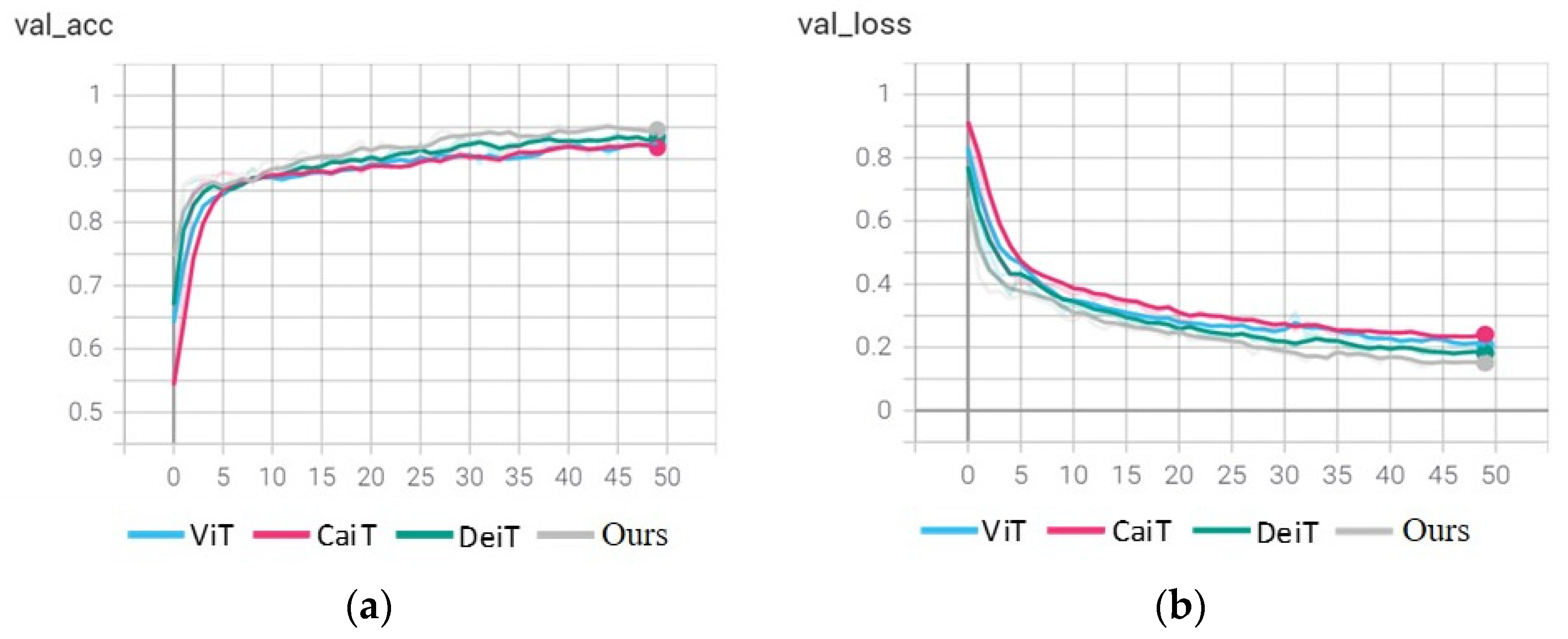
3.3. Comparative Experiments between DeformAtt-ViT and other ViTs

To validate the performance of common ViT models on the task of classifying the hunger degree of fish, we selected three models, ViT, CaiT, and DeiT, to conduct comparative experiments with DeformAtt-ViT. First, we presented comparative graphs of loss and accuracy curves for our DeformAtt-ViT and three transformers. The two sets of comparative experimental tables are shown in Figure 6.

It can be observed that the loss curves of all ViT models gradually decreased and reached a convergence state, while the accuracy curves gradually increased and eventually stabilized. All curves exhibit normal behavior, indicating that the model continuously learns more accurate features. Compared with ViT, CaiT, and DeiT, DeformAtt-ViT had the highest accuracy value and the lowest loss value at the same number of iterations. As shown in Figure 6, after the number of iterations reached 40, the curve of the validation loss value gradually became flattened, indicating that the model was close to convergence. Compared with the other three Transformer models, DeformAtt-ViT had a smoother fluctuation in its loss curve. It demonstrated a better level of model training in the initial stages of iteration, indicating a higher degree of network optimization. Thus, it can be stated that the inclusion of deformable modules in DeformAtt-ViT indeed significantly enhanced the performance of the model, and the network of DeformAtt-ViT was more stable and exhibited good robustness.

We then evaluated the performances of the four models by using the relevant metrics data. As shown in Figure 7, among the four transformer models, both ViT and CaiT exhibited very similar performance in the four metrics, but they were noticeably lower than DeiT and DeformAtt-ViT. DeformAtt-ViT achieved an overall accuracy of 95.50% in fish hunger-degree classification, which was 1.31% higher than the second-best performer (DeiT). Additionally, the precision, recall, and F1-score were 96.58%, 94.17%, and 95.36% respectively, which were all improved compared with other ViT models.

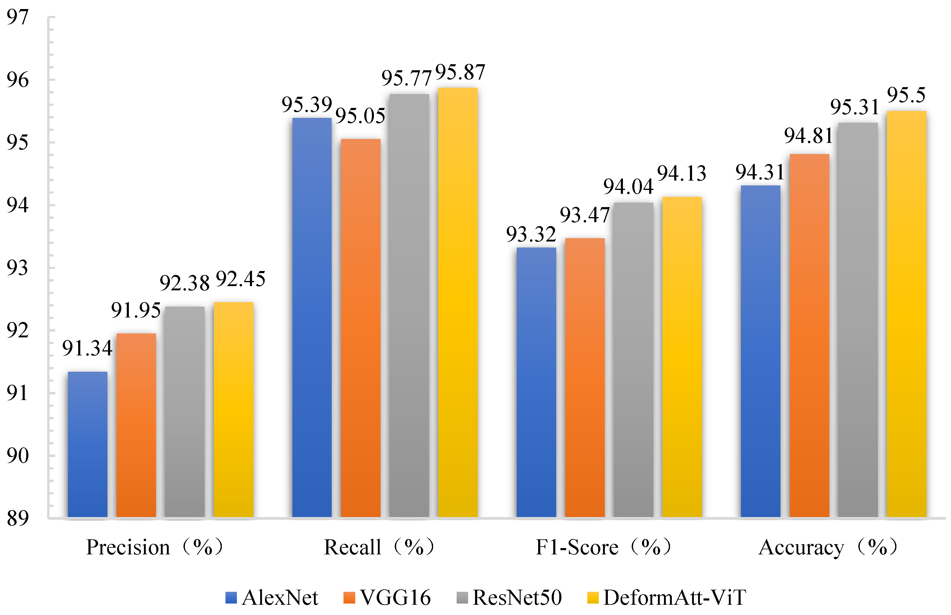
3.4. Comparative Experiments between DeformAtt-ViT and other CNNs

CNN has been widely used in a variety of computer-vision classification tasks due to its inherent good properties. We continued to choose three CNN models as comparative models, including AlexNet, VGG16, and ResNet50 for comparison with DeformAtt-ViT. Graphs of loss and accuracy curves for DeformAtt-ViT and three CNNs are shown in Figure 8. DeformAtt-ViT initially performed well in terms of the accuracy curve, but it was later surpassed by ResNet50 until after the 30th round, when it surpassed again and started to converge. In terms of the loss curve, it can be observed that traditional CNNs had larger loss values during the initial validation stage, but they converged faster, while DeformAtt-ViT had relatively lower values.

The performance evaluation on the four metrics precision, recall, F1-score, and accuracy are shown in Figure 9. As can be seen, among the three CNN models, ResNet50 performed the best in all metrics. The precision, recall, F1-score, and accuracy of ResNet50 were 92.38%, 95.77%, 94.04%, and 95.31% respectively. Additionally, AlexNet, which was the worst-performing model among the three CNN models, also outperformed the other three transformer models in all four metrics, except DeformAtt-ViT. Compared to ResNet50 methods, DeformAtt-ViT showed improvements in all four metrics. DeformAtt-ViT achieved an overall accuracy of 95.50% in fish hunger-degree classification, which is an increase of 0.19%. Additionally, the precision, recall, and F1-score were 96.58%, 94.17%, and 95.36% respectively.

We further compared DeformAtt-ViT with previous publications [14,15,16]. The frameworks of these networks can be referred to in Table S1, while the evaluation results are presented in Figures S3 and S4.

3.5. Model Visualization

To guarantee the robustness of the model, we used Grad-CAM to generate heatmaps for the last layer of the seven models. Grad-CAM is an explainable approach for analyzing the decision-making mechanism of deep-learning models (i.e., to visualize where the deep-learning model is looking). The redder the color, the larger the contribution of the region to the final prediction result will be, while the blue area indicates a weak contribution. From Figure 10, it can be observed that, compared with AlexNet and VGG16, ResNet50 is more focused on detecting overlapping areas of fish shoals and accurately capturing the key features of the fish shoal. On the other hand, ViT showed a more divergent focus in the three classification states. The advantage of ViT lies in its ability to capture long-range dependencies in images without the need for complex convolutional operations [30]. As shown in Figure 10, ViT was better at focusing on small areas where two to three fish congregate. CaiT focused more on the background areas where fish were sparse in the strongly hungry degree. DeiT [31], which is based on ViT and incorporates a distillation token for distillation learning, paid more attention in the hungry degree. In the weakly hungry degree, DeformAtt-ViT had a larger red area, indicating that fish shoals were more dispersed in this state. Through deformable convolutions, DeformAtt-ViT could learn relationships such as the distance between fish shoals. In the two kinds of hunger degrees, several heavily overlapping areas with multiple fish were highlighted, and the feature maps had a better sense of boundaries.

4. Discussion

4.1. Comparison Analysis between CNNs and Transformers

In this study, two popular deep-learning architectures, CNN and transformer, were chosen for comparative evaluation over the established dataset in the fish hunger-degree identification task. In general, the identification accuracy of the proposed DeformAtt-ViT, along with three transformers (ViT, CaiT, and DeiT) and three CNNs (AlexNet, VGG16, and ResNet50), all achieved over 92%, indicating that all models can accurately extract the features of different hunger degrees. Among them, DeformAtt-ViT achieved the optimal performance in regard to all evaluation criteria. The advantageous architecture of DeformAtt-ViT utilized the deformable attention module in Stages 3 and 4 based on the ablation experiment (Table 1). DeformAtt-Vit would focus more on relevant regions (i.e., where the fish objects were located) and identify whether the fish were gathering from a global view, thereby categorizing the fish hunger degree accurately.

It was also worth noting that all three CNNs performed slightly better than ViT, CaiT, and DeiT. This was because the performance of transformers relied on the size of the datasets to be trained. Training vision transformers requires a larger amount of data, with better training results achieved with larger datasets [32]. When insufficient data is provided, the generalization of transformers would be limited. For instance, Li et al. [33] conducted a comparative study on the recognition of 2095 diseased and healthy sugarcane leaves collected in the field environment and found that ResNet50 had a significantly better effect than ViT. Li et al. [34] compared ViTs with ResNet on 7434 sheet face-recognition tasks. The results showed that ResNet-50 performed better than ViT Base but worse than Swin Base. The performance of ViTs and CNN does not entirely depend on the size of the dataset but is closely related to the quality, distribution, application scenarios, and other characteristics of the image dataset itself. For example, Li et al. [35] proposed a specialized medical image-classification model with a visual transformer backbone based on the gap between medical images and natural images.

Meanwhile, the architectures of CNNs and transformers have a major difference [36]. In a CNN, the convolutional kernels can capture local features through local receptive fields and shared weights. However, a vision transformer divides a given image into several patches and assigns a position embedding to each patch. All patches are then flattened by linear projection and transferred to the encoder module. In essence, the vision transformer evaluates the contribution of an individual patch in the whole image when generating the output [37]. Under such a circumstance, more training data is required. Furthermore, a CNN would perform better due to its deep architectures [38]. It can be seen from Figure 9 that ResNet50 achieved the optimal performance among all three CNNs, considering it has 50 layers (49 convolutional layers and 1 fully connected layer) in total. When a CNN has a deep layer, the feature-extraction ability would be greatly enhanced [39]. Usually, shallow layers can capture features like edges and textures, while deep layers are able to extract semantic information.

Compared with ResNet50, DeformAtt-ViT still showed an improvement in precision, recall, F1-score, and accuracy. The success of DeformAtt-ViT was attributed to its unique deformable attention module. The deformable attention ensured that the same receptive field was applied to all queries, and the sampling points were learned through the offset network [40]. Moreover, the offset network leverages query features as inputs to generate corresponding offsets for all reference points. This process effectively shifts the candidate keys and values to important regions, enabling the model to enhance the original self-attention module with greater flexibility and efficiency.

Lastly, considering the use of the attention mechanism, DeformAtt-ViT seemed to be more transparent than CNNs. By visualizing the heatmap generated by the attention mechanism in the given image, highlighted contributing pixels would naturally provide a visual explanation of the decision-making process of the model [41]. In this fish hunger-degree classification task, the deformable attention module was particularly helpful when dealing with the weakly hungry categorization, since fish were generally sparse within the space. From the result in Figure 10a, DeformAtt-ViT successfully looked at multiple objects from a global view with a larger receptive field [42]. However, the feature-extraction ability of CNNs was limited due to the fixed size of convolutional kernels.

4.2. Limitation and Future Work

DeformAtt-ViT has proven to be effective in monitoring the fish-feeding process in recirculating aquaculture systems. DeformAtt ViT can identify the degree of aggregation of fish and then trigger the feeding machine to be turned on. When the aggregation disappears, DeformAtt ViT then suggests stopping the feeding machine. This intelligent and precise feeding approach allows for optimizing the use of feed resources, ensuring efficient aquaculture operations, and reducing production costs. There are also some limitations to be overcome for this study in the future.

First, the feeding dataset was collected in a laboratory setting with relatively small-sized image data. It is crucial to consider that, as the largemouth bass grows, its behavior may change with time. Additionally, fish habits can vary under different conditions, such as water temperature, pH, lighting, and other environmental factors. To address these limitations, future work should involve collecting data in real-life aquacultural environments, evaluating the hunger levels of largemouth bass throughout their entire growth cycle and considering different stress conditions.

Secondly, this study classified the hunger degree of fish based on static 2D feeding images. We acknowledged that image-based and video-based approaches are adopted in the intelligent-feeding research, both of which are important. On the one hand, for the image-based approach adopted in this manuscript, our objective was to detect the aggregation level to determine whether the fish are hungry before the feeding bait is released. Although the image data used in this study was downsampled from videos, we noticed that neighboring video frames might contain redundant information. Inputting a continuous temporal sequence of video frames not only heavies the computational burden but also may affect the mode performance. Therefore, the image-based approach is a preferable option for our study. On the other hand, most of the video-based approaches aim at detecting the feeding intensity of fish after releasing the bait. Also, the behavior analysis under stress (e.g., swimming, cruising, escaping, etc.) needs the support of video-based approaches. For instance, Beyan et al. [43] demonstrated through analysis of 12,247 videos that, as the water temperature increases, the swimming speed of fish increases. Xu et al. [44] analyzed the abnormal behavior trajectory, movement volume, and movement speed of sturgeon, bass, and crucian carp in different stages of acute ammonia nitrogen stress-recovery experiments through video monitoring, in order to alert whether ammonia nitrogen in aquaculture water was abnormal. Conclusively, the image-based and video-based analysis approaches have different objectives. However, intelligent feeding is a complex and dynamic process. Integrating both approaches can potentially enrich the functionality of the intelligent feeding system and improve the system’s performance [45]. We have initiated preliminary experiments by employing YOLOv8 in conjunction with the ByteTrack object-tracking algorithm to track both aggregated and relatively stationary states, as well as normal swimming states. The results are shown in Figure S5. It could be observed that the consecutive frames extracted in Figure S5a indicated that the fish were relatively stationary, as evidenced by the lack of significant movement in the motion trajectories of the fish. In contrast, the consecutive frames in Figure S5b showed that most of the fish were in a normal swimming state, such as fish with the identification numbers 1, 12, and 26, exhibiting distinct changes in their motion trajectories. Additionally, studies have shown that the sound produced by fish during feeding can also quantify their feeding behavior [23]. Therefore, fusing multiple data sources can lead to more reliable and effective decision-making for the feeding process.

Furthermore, although deep-learning models with deep layers have the potential to achieve promising results, they may require more training time. Considering that the deployment of models on edge devices with limited computational capabilities is becoming increasingly important, there is a growing trend toward designing lightweight networks [46].

5. Conclusions

This study focused on the practical requirements of fish feeding, specifically targeting largemouth bass. DeformAtt-ViT, serving as a reference model, was compared with six other models in the classification task of fish hunger degree. The main findings of the paper are as follows. We validated that deformable attention was capable of effectively filtering out irrelevant information and enhancing the utilization of useful information through an ablation study. As a result, it guides the model to prioritize more significant regions. The performance of the results demonstrated that DeformAtt-ViT outperformed the other models, achieving a classification accuracy of 95.5%. To further evaluate the effectiveness of the models, we generated visual heat maps using the Grad-CAM method. These heat maps specifically highlighted the regions of interest that are crucial for determining the hunger degree of fish. The findings of this study have significant implications for the establishment of intelligent feeding systems and the reduction of fish-feeding costs. They also offer valuable guidance for researchers in model selection and optimization for similar tasks. By leveraging the insights gained from this research, future studies can enhance the accuracy and efficiency of fish-feeding systems, leading to improved aquaculture practices.

References

1. FAO. The State of World Fisheries and Aquaculture 2022; Food and Agriculture Organization of the United Nations (FAO): Rome, Italy, 2022. [Google Scholar] [CrossRef]
2. Yang, L.; Liu, Y.; Yu, H.; Fang, X.; Song, L.; Li, D.; Chen, Y. Computer Vision Models in Intelligent Aquaculture with Emphasis on Fish Detection and Behavior Analysis: A Review. Arch. Comput. Methods Eng. 2021, 28, 2785–2816. [Google Scholar] [CrossRef]
3. Zhou, C.; Xu, D.; Lin, K.; Sun, C.; Yang, X. Intelligent feeding control methods in aquaculture with an emphasis on fish: A review. Rev. Aquac. 2018, 10, 975–993. [Google Scholar] [CrossRef]
4. Yang, X.; Zhang, S.; Liu, J.; Gao, Q.; Dong, S.; Zhou, C. Deep learning for smart fish farming: Applications, opportunities and challenges. Rev. Aquac. 2021, 13, 66–90. [Google Scholar] [CrossRef]
5. Wang, C.; Li, Z.; Wang, T.; Xu, X.; Zhang, X.; Li, D. Intelligent fish farm—The future of aquaculture. Aquac. Int. 2021, 29, 2681–2711. [Google Scholar] [CrossRef]
6. Li, D.; Wang, Z.; Wu, S.; Miao, Z.; Du, L.; Duan, Y. Automatic recognition methods of fish feeding behavior in aquaculture: A review. Aquaculture 2020, 528, 735508. [Google Scholar] [CrossRef]
7. Wang, H.; Zhang, S.; Zhao, S.; Lu, J.; Wang, Y.; Li, D.; Zhao, R. Fast detection of cannibalism behavior of juvenile fish based on deep learning. Comput. Electron. Agric. 2022, 198, 107033. [Google Scholar] [CrossRef]
8. Feng, S.; Yang, X.; Liu, Y.; Zhao, Z.; Liu, J.; Yan, Y.; Zhou, C. Fish feeding intensity quantification using machine vision and a lightweight 3D ResNet-GloRe network. Aquac. Eng. 2022, 98, 102244. [Google Scholar] [CrossRef]
9. Michael, S.C.J.; Patman, J.; Lutnesky, M.M.F. Water clarity affects collective behavior in two cyprinid fishes. Behav. Ecol. Sociobiol. 2021, 75, 120. [Google Scholar] [CrossRef]
10. Kramer, D.L. Dissolved oxygen and fish behavior. Environ. Biol. Fish. 1987, 18, 81–92. [Google Scholar] [CrossRef]
11. Volkoff, H.; Rønnestad, I. Effects of temperature on feeding and digestive processes in fish. Temperature 2020, 7, 307–320. [Google Scholar] [CrossRef]
12. Assan, D.; Huang, Y.; Mustapha, U.F.; Addah, M.N.; Li, G.; Chen, H. Fish feed intake, feeding behavior, and the physiological response of apelin to fasting and refeeding. Front. Endocrinol. 2021, 12, 798903. [Google Scholar] [CrossRef] [PubMed]
13. Wu, Y.; Wang, X.; Zhang, X.; Shi, Y.; Li, W. Locomotor posture and swimming-intensity quantification in starvation-stress behavior detection of individual fish. Comput. Electron. Agric. 2022, 202, 107399. [Google Scholar] [CrossRef]
14. Iqbal, U.; Li, D.; Akhter, M. Intelligent Diagnosis of Fish Behavior Using Deep Learning Method. Fishes 2022, 7, 201. [Google Scholar] [CrossRef]
15. Zhu, M.; Zhang, Z.; Huang, H.; Chen, Y.; Liu, Y.; Dong, T. Classification of perch ingesting condition using light-weight neural network MobileNetV3-Small. Nongye Gongcheng Xuebao/Trans. Chin. Soc. Agric. Eng. 2021, 37, 165–172. [Google Scholar] [CrossRef]
16. Zhou, C.; Xu, D.; Chen, L.; Zhang, S.; Sun, C.; Yang, X.; Wang, Y. Evaluation of fish feeding intensity in aquaculture using a convolutional neural network and machine vision. Aquaculture 2019, 507, 457–465. [Google Scholar] [CrossRef]
17. Simonyan, K.; Zisserman, A. Very Deep Convolutional Networks for Large-Scale Image Recognition. arXiv 2014, arXiv:1409.1556. [Google Scholar] [CrossRef]
18. He, K.; Zhang, X.; Ren, S.; Sun, J. Deep Residual Learning for Image Recognition. In Proceedings of the IEEE Computer Society Conference on Computer Vision and Pattern Recognition (CVPR), Las Vegas, NV, USA, 27–30 June 2016; pp. 770–778. [Google Scholar] [CrossRef]
19. Chen, J.; Huang, H.; Cohn, A.G.; Zhou, M.; Zhang, D.; Man, J. A hierarchical DCNN-based approach for classifying imbalanced water inflow in rock tunnel faces. Tunn. Undergr. Space Technol. 2022, 122, 104399. [Google Scholar] [CrossRef]
20. Vaswani, A.; Shazeer, N.; Parmar, N.; Uszkoreit, J.; Jones, L.; Gomez, A.N.; Kaiser, L.; Polosukhin, I. Attention Is All You Need. arXiv 2017, arXiv:1706.03762. [Google Scholar] [CrossRef]
21. Bashmal, L.; Bazi, Y.; Al Rahhal, M.M.; Alhichri, H.; Al Ajlan, N. UAV Image Multi-Labeling with Data-Efficient Transformers. Appl. Sci. 2021, 11, 3974. [Google Scholar] [CrossRef]
22. Li, W.; Liu, Y.; Wang, W.; Li, Z.; Yue, J. TFMFT: Transformer-based multiple fish tracking. Comput. Electron. Agric. 2024, 217, 108600. [Google Scholar] [CrossRef]
23. Zeng, Y.; Yang, X.; Pan, L.; Zhu, W.; Wang, D.; Zhao, Z.; Liu, J.; Sun, C.; Zhou, C. Fish school feeding behavior quantification using acoustic signal and improved Swin Transformer. Comput. Electron. Agric. 2023, 204, 107580. [Google Scholar] [CrossRef]
24. Xia, Z.; Pan, X.; Song, S.; Li, L.E.; Huang, G. Vision Transformer with Deformable Attention. arXiv 2022, arXiv:2201.00520. [Google Scholar] [CrossRef]
25. Zhou, B.; Yu, X.; Liu, J.; An, D.; Wei, Y. Effective Vision Transformer Training: A Data-Centric Perspective. arXiv 2022, arXiv:2209.15006. [Google Scholar] [CrossRef]
26. Dong, X.; Bao, J.; Chen, D.; Zhang, W.; Yu, N.; Yuan, L.; Chen, D.; Guo, B. CSWin Transformer: A General Vision Transformer Backbone with Cross-Shaped Windows. arXiv 2021, arXiv:2107.00652. [Google Scholar] [CrossRef]
27. Liu, Z.; Lin, Y.; Cao, Y.; Hu, H.; Wei, Y.; Zhang, Z.; Lin, S.; Guo, B. Swin Transformer: Hierarchical Vision Trans-former using Shifted Windows. arXiv 2021, arXiv:2103.14030. [Google Scholar] [CrossRef]
28. Dai, J.; Qi, H.; Xiong, Y.; Li, Y.; Zhang, G.; Hu, H.; Wei, Y. Deformable Convolutional Networks. arXiv 2017, arXiv:1703.06211. [Google Scholar] [CrossRef]
29. Selvaraju, R.R.; Cogswell, M.; Das, A.; Vedantam, R.; Parikh, D.; Batra, D. Grad-CAM: Visual Explanations from Deep Networks via Gradient-Based Localization. Int. J. Comput. Vis. 2016, 128, 336–359. [Google Scholar] [CrossRef]
30. Tuli, S.; Dasgupta, I.; Grant, E.; Griffiths, T.L. Are Convolutional Neural Networks or Transformers more like human vision? arXiv 2021, arXiv:2105.07197. [Google Scholar] [CrossRef]
31. Touvron, H.; Cord, M.; Douze, M.; Massa, F.; Sablayrolles, A.; Jégou, H. Training data-efficient image transformers & distillation through attention. arXiv 2020, arXiv:2012.12877. [Google Scholar] [CrossRef]
32. Dosovitskiy, A.; Beyer, L.; Kolesnikov, A.; Weissenborn, D.; Zhai, X.; Unterthiner, T.; Dehghani, M.; Minderer, M.; Heigold, G.; Gelly, S.; et al. An Image is Worth 16x16 Words: Transformers for Image Recognition at Scale. arXiv 2020, arXiv:2010.11929. [Google Scholar] [CrossRef]
33. Li, X.; Li, X.; Zhang, M.; Dong, Q.; Zhang, G.; Wang, Z.; Wei, P. SugarcaneGAN: A novel dataset generating approach for sugarcane leaf diseases based on lightweight hybrid CNN-Transformer network. Comput. Electron. Agric. 2024, 219, 108762. [Google Scholar] [CrossRef]
34. Li, X.; Xiang, Y.; Li, S. Combining convolutional and vision transformer structures for sheep face recognition. Comput. Electron. Agric. 2023, 205, 107651. [Google Scholar] [CrossRef]
35. Li, Y.; Huang, Y.; He, N.; Ma, K.; Zheng, Y. Improving vision transformer for medical image classification via token-wise perturbation. J. Vis. Commun. Image Represent. 2023, 98, 104022. [Google Scholar] [CrossRef]
36. Xiong, B.; Chen, W.; Niu, Y.; Gan, Z.; Mao, G.; Xu, Y. A Global and Local Feature fused CNN architecture for the sEMG-based hand gesture recognition. Comput. Biol. Med. 2023, 166, 107497. [Google Scholar] [CrossRef]
37. Zhou, D.; Kang, B.; Jin, X.; Yang, L.; Lian, X.; Jiang, Z.; Hou, Q.; Feng, J. DeepViT: Towards Deeper Vision Trans-former. arXiv 2021, arXiv:2103.11886. [Google Scholar] [CrossRef]
38. Asswin, C.R.; KS, D.K.; Dora, A.; Ravi, V.; Sowmya, V.; Gopalakrishnan, E.A.; Soman, K.P. Transfer learning approach for pediatric pneumonia diagnosis using channel attention deep CNN architectures. Eng. Appl. Artif. Intell. 2023, 123, 106416. [Google Scholar] [CrossRef]
39. Lin, T.-Y.; Dollár, P.; Girshick, R.; He, K.; Hariharan, B.; Belongie, S. Feature Pyramid Networks for Object Detection. arXiv 2017, arXiv:1612.03144. [Google Scholar] [CrossRef]
40. Jiang, X.; Li, Y.; Jiang, T.; Xie, J.; Wu, Y.; Cai, Q.; Jiang, J.; Xu, J.; Zhang, H. RoadFormer: Pyramidal deformable vision transformers for road network extraction with remote sensing images. Int. J. Appl. Earth Obs. Geoinf. 2022, 113, 102987. [Google Scholar] [CrossRef]
41. Gong, B.; Dai, K.; Shao, J.; Jing, L.; Chen, Y. Fish-TViT: A novel fish species classification method in multi water areas based on transfer learning and vision transformer. Heliyon 2023, 9, e16761. [Google Scholar] [CrossRef]
42. Yang, W.; Wu, J.; Zhang, J.; Gao, K.; Du, R.; Wu, Z.; Firkat, E.; Li, D. Deformable convolution and coordinate attention for fast cattle detection. Comput. Electron. Agric. 2023, 211, 108006. [Google Scholar] [CrossRef]
43. Beyan, C.; Fisher, R.B.; Katsageorgiou, V.-M. Extracting statistically significant behaviour from fish tracking data with and without large dataset cleaning. IET Comput. Vis. 2018, 12, 162–170. [Google Scholar] [CrossRef]
44. Xu, W.; Liu, C.; Wang, G.; Zhao, Y.; Yu, J.; Muhammad, A.; Li, D. Behavioral response of fish under ammonia nitrogen stress based on machine vision. Eng. Appl. Artif. Intell. 2024, 128, 107442. [Google Scholar] [CrossRef]
45. Wang, Y.; Yu, X.; Liu, J.; Zhao, R.; Zhang, L.; An, D.; Wei, Y. Research on quantitative method of fish feeding activity with semi-supervised based on appearance-motion representation. Biosyst. Eng. 2023, 230, 409–423. [Google Scholar] [CrossRef]
46. Kim, W.; Jung, W.-S.; Choi, H.K. Lightweight Driver Monitoring System Based on Multi-Task Mobilenets. Sensors 2019, 19, 3200. [Google Scholar] [CrossRef] [PubMed]
Figure 1. Data-collection schematics.
Jmse 12 00726 g001
Figure 2. Three hunger degrees of fish samples. (a) weakly hungry; (b) moderately hungry; and (c) strongly hungry.
Jmse 12 00726 g002
Figure 3. DeformAtt-ViT architecture. Note: Stage 1 to Stage 4 are the stacked successive local attention, shift-window, and deformable attention blocks. k and s indicate the kernel size and stride. H, W, and C indicate the height, width, and channels.
Jmse 12 00726 g003
Figure 4. Deformable attention module.
Jmse 12 00726 g004
Figure 5. The shifted-window approach.
Jmse 12 00726 g005
Figure 6. Evaluation of four models: (a) the accuracy change curve of ViT, CaiT, Deit, and DeformAtt-ViT; (b) the loss value change curve of ViT, CaiT, Deit, and DeformAtt-ViT.
Jmse 12 00726 g006
Figure 7. Comparison of accuracy, recall, F1-score, and accuracy between ViT, CaiT, DeiT and DeformAtt-ViT.
Jmse 12 00726 g007
Figure 8. Evaluation of four models: (a) the accuracy change curve of AlexNet, VGG16, ResNet50 and DeformAtt-ViT; (b) the loss value change curve of AlexNet, VGG16, ResNet50 and DeformAtt-ViT.
Jmse 12 00726 g008
Figure 9. Comparison of accuracy, recall, F1-score, and accuracy between AlexNet, VGG16, ResNet50 and DeformAtt-ViT.
Jmse 12 00726 g009
Figure 10. Heat maps of seven networks of three hunger degrees. (a) illustrates the visual heat map for the weakly hungry degree, (b) displays the heat map for the moderately hungry degree, and (c) showcases the heat map for the strongly hungry degree. All the original input images were selected randomly for this analysis.
Jmse 12 00726 g010