Article

Nonparametric Modelling of Ship Dynamics Using Puma Optimizer Algorithm-Optimized Twin Support Vector Regression

1
College of Intelligent Systems Science and Engineering, Harbin Engineering University, Harbin 150009, China
2
Nanjing Research Institute of Electronic Engineering, Nanjing 210007, China
*
Author to whom correspondence should be addressed.
J. Mar. Sci. Eng. 2024, 12(5), 754; https://doi.org/10.3390/jmse12050754
Submission received: 24 March 2024 / Revised: 25 April 2024 / Accepted: 29 April 2024 / Published: 30 April 2024

Abstract

:
Ship dynamic models serve as the foundation for designing ship controllers, trajectory planning, and obstacle avoidance. Support vector regression (SVR) is a commonly used nonparametric modelling method for ship dynamics. Achieving high accuracy SVR models requires a substantial amount of training samples. Additionally, as the number of training samples increases, the computational efficiency for solving the quadratic programming problem (QPP) of SVR decreases. Ship controllers demand dynamic models with both high accuracy and computational efficiency. Therefore, to enhance the prediction accuracy and computational efficiency of SVR, this paper proposes a nonparametric modelling method based on twin SVR (TSVR). TSVR replaces a large QPP with a set of smaller QPPs, significantly enhancing generalizability and computational efficiency. To further improve the predictive accuracy of TSVR, the puma optimizer algorithm is employed to determine the optimal hyperparameters. The performance of the proposed method is validated using a Mariner class vessel. Gaussian white noise is introduced into the modelling data to simulate measurement error. The TSVR model accurately predicts various zigzag and turning circle manoeuvring motions under disturbance conditions, demonstrating its robustness and generalizability. Compared to the SVR model, the TSVR model achieves lower root mean square error and computational time, confirming its superior predictive accuracy and computational efficiency.

1. Introduction

The accuracy of ship dynamic models is crucial for analysing ship manoeuvring characteristics, ship controller design, and trajectory planning [1]. However, due to the high complexity and coupling of ship motion, obtaining accurate and reliable ship dynamic models is extremely challenging. Additionally, the design of ship controllers requires ships to update their models or perform online modelling based on external environmental changes [2]. This necessitates ship dynamic models to possess both high accuracy and computational efficiency, further increasing the modelling complexity.
Existing methods for ship dynamics modelling can be categorized into mechanistic modelling and data-driven modelling [3]. Mechanistic modelling aims to obtain a mathematical model of ship motion. Its kinematic model describes the relative relationships of the ship in multiple coordinate systems [4]. The dynamic model formulates hydrodynamic forces/moments, control forces, and environmental disturbances acting on the hull [5]. The parameters in the dynamic model, known as hydrodynamic derivatives, are obtained through a Taylor expansion of the state variables [6]. There are various methods to determine the specific values of these parameters, such as computational fluid dynamics, captive model tests, and empirical formulas or databases [7]. However, when determining a large number of hydrodynamic derivatives, these methods suffer from issues such as high computational costs, significant time consumption, or low accuracy [8]. Moreover, mechanistic modelling methods require a significant amount of prior knowledge (e.g., ship dynamics and ship kinematics), which further increases the complexity of modelling [9].
Data-driven modelling is the latest modelling approach developed through machine learning techniques. Compared to mechanistic models, data-driven modelling requires less prior knowledge [10]. This method offers lower computational costs and higher modelling efficiency. System identification (SI) is the primary method of data-driven modelling. SI does not require complex tank experiments to obtain hydrodynamic derivative values but instead models using data collected from free-running model tests or full-scale trials [11]. Parametric modelling is a direct and widely used method of SI modelling [12,13]. To capture the six-degree-of-freedom (DOF) dynamics of ships, Zhu et al. [14] designed a simplified parametric model. The hydrodynamic derivatives within the parametric model are identified through support vector regression (SVR). Chen et al. [15] constructed a parametric model for a four-DOF container ship using a least squares SVR (LSSVR) for SI. The robustness of this parametric model was validated under multilevel noise interference. Sutulo and Guedes Soares [16] designed a Hausdorff metric loss function combined with a genetic algorithm to reduce the impact of noise on the parametric model. Yadollah Sajedi and Mohammad Bozorg [17] designed a robust extended Kalman filter (EKF) and an extended H-infinity filter and applied them to identify autonomous underwater vehicles. Perera et al. [18] suggested that unstructured uncertainty is associated with the improved turning model when applying the EKF for model identification. Padilla et al. [19] proposed two methods for identifying continuous-time ship dynamic models using real data obtained from rivers. The first method involves identification through optimization using disturbance observers. The second method corresponds to the modified auxiliary variable method for linear time-varying systems. Muske et al. [20] identified a nonlinear dynamic model of an unmanned vessel using parameter estimation data from towing experiments. Haro Casado et al. [21] proposed a four-parameter identification algorithm for ship models based on adaptive processes and backstepping theory. This work makes a contribution to solving the problem of parameter identification for ship models based on experimental results. During turning experiments, only knowledge of the ship’s turning radius is required for identification. Ibrahim et al. [22] established the inherent nonlinear motion control equations of ships for studying the dynamic behaviour of ships navigating in adverse environments. They include an assessment of roll stochastic stability and probabilistic approaches used to estimate the probability of capsizing and parameter identification. Phairoh et al. [23] updated the parameters of a linear roll model using system identification methods when the ship’s dynamics changed. Numerical simulation results show that generalized predictive control performs optimally in controlling ship roll motion. Parametric modelling relies on prior knowledge of the model structure and input–output data [24]. The four commonly used model structures are the Abkowitz model [25], the manoeuvring modelling group model [26], the Fossen model [5], and the response model [27]. The first three types of model structures all have the capability to capture ship dynamics. However, due to the highly coupled and nonlinear nature of ship motion, a large number of parameters need to be identified. Moreover, the presence of parameter drift makes accurately identifying these parameters very challenging [3]. The response model, on the other hand, is simple in form and easy to implement. However, it cannot fully simulate ship motion, and its predictive accuracy needs improvement [28]. Therefore, choosing the appropriate model structure is very challenging even for experienced modellers.
The nonparametric modelling (black-box modelling) is another modelling method in SI [29]. This approach does not require the selection of complex model structures but relies on input and output data to construct a nonlinear function to describe ship dynamic information, which increases modelling efficiency [24]. Black-box modelling has been widely applied in ship dynamic modelling. Zongkai et al. [30] addressed the issue of constructing ship dynamic models typically using model ships or simulated data by proposing a nonparametric ship dynamic model based on real ship voyage data. The results demonstrate the feasibility and practical value of the ship dynamic model. Moreno et al. [31] established general and robust black-box models using real experimental data from random motion and identified them using ridge, kernel ridge, and symbolic regression techniques. The results prove that machine learning techniques are robust approaches to model surface marine vehicles. Moreno-Salinas et al. [32] utilized kernel ridge regression and kernel ridge regression confidence machine to model unmanned vessels. The model reproduces ship behaviour with significant accuracy, and the model response is within the confidence interval. Skulsad et al. [33] proposed a tool for ship-based support based on integrating machine learning models of ships into ship dynamic models to provide position predictions. Machine learning models are applied as compensators for inaccuracies in the dynamic model. Experimental results show that the inclusion of data-driven machine learning models significantly improves prediction accuracy. Diez et al. [34] proposed and discussed a data-driven, equation-independent ship wave manoeuvring response prediction method based on dynamic mode decomposition. It provides a finite-dimensional representation of nonlinear system dynamics through a set of modes with associated oscillation frequencies and decay/growth rates. It allows for short-term future estimates of system states and can be used for real-time prediction and control. Prediction results for the heading keeping of the 5415 M Navy destroyer in irregular stern waves and the turning motion of the KRISO container ship in regular waves demonstrate the effectiveness of this model. Xue et al. [35] designed a Gaussian process regression model to consider the impact of uncertainty in ship dynamics modelling. The effectiveness of the model was validated through a database of ship manoeuvring simulation methods. Wang et al. [7] employed nu-SVR to identify the dynamics model for a KVLCC2 vessel. The model utilized a radial basis function (RBF) kernel, and the hyperparameter values were determined through a designed optimization method. Zhang et al. [29] employed a random excitation signal as training data to optimize the performance of a dynamic model of Mariner vessels. Additionally, Zhang et al. designed a multioutput nu-SVR for the identification of the dynamics model. Luo et al. [36] utilized SVR for dynamic modelling of a catamaran. In the modelling process, the influence of environmental disturbances (e.g., wind and currents) on ship dynamics is considered. Jiang et al. [24] employed multioutput LSSVR for modelling a container ship. The multioutput LSSVR considers the correlation and differences among four-DOF state variables. The prior information of nonparametric modelling includes only training data and input–output features [37]. The training data are collected through onboard sensors from free-running model tests or full-scale trials. Input–output features are selected based on the ship’s dynamics to choose relevant variables for the state variables. Due to its ease of implementation and high accuracy, it has become the preferred modelling method for unknown model structures [38].
There are many methods that can be used for ship dynamic nonparametric modelling, such as artificial neural network (ANN) [39] and SVR [7,11,24,29]. ANN is based on traditional statistical theory and is suitable for large-sample regression fitting. However, when it comes to modelling ship dynamics with small sample sizes, ANN often encounters issues such as local optima and slow training speeds [7]. SVR is a machine learning method proposed by Vapnik [40] based on the Vapnik–Chervonenkis dimension and statistical learning. Compared to ANN, SVR is better at handling small-sample regression problems and is less prone to getting trapped in local optima [7]. SVR aims to find a hyperplane to fit the training data. During the training process of SVR, quadratic programming problems (QPPs) need to be solved to obtain the optimal solution of the dual problem [41]. However, the computation time of the QPPs increases with increasing training sample size. This decreases the computational efficiency of SVR [42]. In the design stage of modern ship controllers, high-precision and -computational efficiency ship dynamic models are required [43]. This requires that the SVR model improve its robustness, generalizability, prediction accuracy, and computational efficiency. Twin SVR (TSVR) is a variant of SVR proposed by Peng [44] in 2010. Unlike SVR, TSVR aims to find two nonparallel hyperplanes to fit the training data. This generates a pair of small-scale QPPs during the training process, each of which determines a constrained bound function. The final prediction value is the average of the predicted values of the two decision functions. Compared to SVR, TSVR has better fitting ability and less training time [45]. Additionally, TSVR also has better generalization ability than SVR [46]. TSVR has been widely applied in various fields, including wind speed forecasting [47], PH prediction [48], potato yield prediction [49], financial time series forecasting [50], and feature selection [51]. Therefore, TSVR has the potential to be used for nonparametric modelling in ship dynamics.
To improve the computational efficiency and accuracy of ship dynamic models, this paper proposes a nonparametric modelling method based on TSVR. TSVR is employed to construct a three-DOF dynamics black-box model for ship manoeuvring motion. The RBF kernel is utilized in the construction of the TSVR model. The optimal hyperparameter values of TSVR are determined by a puma optimizer (PO) algorithm [52]. The effectiveness and robustness of the proposed algorithm are validated through simulation on a Mariner class vessel.
The remainder of the paper is organized as follows: Section 2 describes ship kinematics and implicit ship dynamics. Section 3 introduces SVR, TSVR, hyperparameter optimization, and modelling processes. In Section 4, the Mariner class vessel is identified based on simulation. The conclusion is summarized in Section 5.

2. Problem Formulation

This study focuses on the 3-DOF dynamics model of surface ships, which primarily encompassing surge speed u , sway speed v , and yaw rate r . Figure 1 illustrates the Earth-fixed coordinate system X O Y and the body-fixed coordinate system x o o y o of a surface ship. Here, ψ , δ , and U are the heading angle, rudder angle, and instantaneous ship speed, respectively.
The kinematic model [6] of the ship is represented by Equation (1):
X ˙ = u cos ψ v sin ψ Y ˙ = u sin ψ + v cos ψ ψ ˙ = r
where X ˙ , etc., are the accelerations of the X , etc.
Based on considerations of ship manoeuvring motion dynamics [7], the 3-DOF dynamics model of the ship can be implicitly represented as Equation (2):
u ˙ = f 1 ( u , v , r , δ ) v ˙ = f 2 ( u , v , r , δ ) r ˙ = f 3 ( u , v , r , δ )
where f i ( ) , i = 1, 2, and 3 are the nonlinear mappings of ship dynamics. Equation (2) can be reformulated as a discrete form:
u ˙ t = f 1 ( x t ) = f 1 ( u t , v t , r t , δ t ) v ˙ t = f 2 ( x t ) = f 2 ( u t , v t , r t , δ t ) r ˙ t = f 3 ( x t ) = f 3 ( u t , v t , r t , δ t )
where t is the time step. x t is the input vector of f i ( ) at the t time step. Equation (3) is selected as the black-box model for the nonparametric modelling of ship dynamics.

3. Twin Support Vector Regression Method

3.1. Support Vector Regression Method

SVR is a commonly used nonparametric modelling method for ship dynamics [7]. SVR is a regression method proposed based on the Vapnik–Chervonenkis dimension and statistical learning [15]. It aims to find a hyperplane to fit training data. This section presents the basic principles of SVR. Given training samples X , y = x i , y i i = 1 n , x i = [ u i , v i , r i , δ i ] T represents the input vector. y i = u ˙ i   v ˙ i , or r ˙ i represents the output responses corresponding to f 1 , f 2 , or f 3 , respectively. n is the number of training samples. The nonlinear SVR needs to find a regression hyperplane (regression function):
f ( x ) = w T φ ( x ) + b
where f = f 1 , f 2 , or f 3 . w is the weighting vector. b is the bias. φ ( ) is a nonlinear mapping. The unknown parameter values within Equation (4) are determined by solving the following minimization problem:
min w , b , ξ , η 1 2 w T w + c ( l T ξ + l T η ) s . t .   y ( φ ( X ) w + l b ) ε l + ξ ( φ ( X ) w + l b ) y ε l + η ξ i 0 , η i 0
where c and ε are the hyperparameters. ξ = [ ξ 1 , , ξ i , , ξ n ] T and η = [ η 1 , , η i , , η n ] T are the slack vectors. l is a unit vector. φ ( X ) = [ φ ( x 1 ) T ; ; φ ( x n ) T ] .
By introducing Lagrange multipliers α = [ α 1 , , α i , , α n ] T and β = [ β 1 , , β i , , β n ] T and using the Karush–Kuhn–Tucker (KKT) conditions, the following dual problem can be obtained:
max α , β 1 2 ( α β ) T k ( X , X T ) ( α β ) ε l T ( α + β ) + y T ( α β ) s . t .   l T ( α β ) = 0 0 l α ,   β c l
where k ( ) is a kernel function. k ( X , X T ) = ( φ ( X ) φ ( X T ) ) is a kernel matrix. ( ) is a dot product operator. In this paper, RBF is used as the kernel function, and its expression is as follows:
k ( x , x i ) = exp ( γ x x i 2 )
where γ is a width hyperparameter. After obtaining the solution to Equation (6), the nonlinear regression function of SVR can be written in the following form:
f ( x ) = i = 1 n ( α i β i ) k ( x , x i ) + b

3.2. TSVR Method

TSVR is an efficient regression algorithm proposed by Peng [44]. TSVR generates two nonparallel hyperplanes (regression functions), corresponding to the ε 1 -insensitive down-bound regressor f 1 ( ) and ε 2 -insensitive up-bound regressor f 2 ( ) , respectively [45]. Compared to SVR, TSVR only needs to solve a pair of small-scale QPPs. The advantage of this approach is that it not only reduces training time but also improves generalizability [46]. The f 1 ( ) and f 2 ( ) can be formulated as:
f 1 ( x ) = k ( x T , X T ) w 1 + b 1 f 2 ( x ) = k ( x T , X T ) w 2 + b 2
where w 1 , w 2 , b 1 , and b 2 are the weightings and bias, respectively. The unknown parameters within Equation (9) need to be solved using the following pair of minimization problems:
min w 1 , b 1 , ξ 1 2 ( y l ε 1 ( k ( X , X T ) w 1 + l b 1 ) ) T     ( y l ε 1 ( k ( X , X T ) w 1 + l b 1 ) ) + c 1 l T ξ s . t .   y ( k ( X , X T ) w 1 + l b 1 ) l ε 1 ξ , ξ i 0 min w 2 , b 2 , η 1 2 ( y + l ε 2 ( k ( X , X T ) w 2 + l b 2 ) ) T     ( y + l ε 2 ( k ( X , X T ) w 2 + l b 2 ) ) + c 2 l T η s . t .   ( k ( X , X T ) w 2 + l b 2 ) y l ε 2 η , η i 0
where c 1 and c 2 are the hyperparameters. ε 1 = ε 2 = 10 4 .
By introducing the Lagrange multipliers α and β and using the KKT conditions, the following dual problem can be obtained:
max α 1 2 α T H ( H T H ) 1 H T α + g T H ( H T H ) 1 H T α g T α s . t .   0 l α c 1 l max β 1 2 β T H ( H T H ) 1 H T β h T H ( H T H ) 1 H T β + h T β s . t .   0 l β c 2 l
where H = [ k ( X , X T ) l ] , g = y l ε 1 , and h = y + l ε 2 . After solving Equation (11), the unknown parameters within Equation (9) can be represented as:
[ w 1 T b 1 ] T = ( H T H ) 1 H T ( g α ) [ w 2 T b 2 ] T = ( H T H ) 1 H T ( h + β )
Finally, the nonlinear regression function of TSVR is obtained as follows:
f ( x ) = 1 2 ( f 1 ( x ) + f 2 ( x ) ) = 1 2 k ( x T , X T ) ( w 1 + w 2 ) + 1 2 ( b 1 + b 2 )

3.3. Hyperparameter Optimization

The performance of TSVR is influenced by its hyperparameters. Specifically, the hyperparameters c 1 , c 2 , and γ control the complexity and accuracy of the model [7]. To enhance the accuracy and generalizability of TSVR, it is necessary to choose appropriate combinations of hyperparameter values. The mean square error (MSE) is a metric for measuring the prediction accuracy [11]. In this paper, MSE is used as the objective function to adjust the hyperparameters:
min μ 1 n v i = 1 n v ( y i y ^ i ( μ ) )
where n v is the number of validation samples. The validation samples and training samples are independent of each other. This approach is used to adjust hyperparameters to enhance the model’s generalizability. y i and y ^ i are the output response and predicted value, respectively. μ = [ c 1 , c 2 , γ ] is the hyperparameter vector to be optimized.
There are many methods that can be used to solve the optimization problem shown in Equation (14). Optimization algorithms are efficient solving methods and have been used for hyperparameter optimization in ship dynamic modelling [6,8,24]. The PO algorithm [52] is a metaheuristic optimization algorithm inspired by the hunting behaviour of pumas. It utilizes different operators for exploitation and exploration phases. These operators can accurately determine the global optimal solution for various optimization problems while achieving rapid convergence speed. Currently, the PO algorithm has been applied to 23 standard functions and 4 machine learning optimization problems [52]. In this paper, the PO algorithm is used to optimize the hyperparameter vector μ . Its initial parameter settings are as follows: the population size is 30, the number of iterations is 500, the search lower bound is [ 0 , 0 , 0 ] , and the search upper bound is [ 100 , 100 , 1 ] .

3.4. Modelling Process

The ship dynamic modelling based on nonparametric modelling methods involves three steps [6,7,8]. Figure 2 illustrates the nonparametric modelling process. The first step is to train the TSVR model based on the training dataset. The training dataset is typically collected from free-running model tests or full-scale trials. TSVR generates a pair of nonparallel hyperplanes to fit these training data. The second step is to optimize hyperparameters based on the validation dataset. There are three hyperparameters μ = [ c 1 , c 2 , γ ] in TSVR that significantly impact model performance. This paper employs the PO algorithm to optimize the numerical combinations of hyperparameters. MSE is selected as a fitness function. The optimization process is conducted on the validation dataset to enhance the model’s generalizability. Once the PO algorithm finds the optimal hyperparameters or reaches the maximum number of iterations, the optimization process finishes. The last step is to conduct free-run simulations. In this process, the initial values of the state variables are given ( u k , v k , r k , ψ k , X k , Y k , k = 0 ). At k time step ( k 0 ), the rudder angle δ k is determined based on experimental requirements (such as zigzag or turning circle experiments) or provided by the controller. The accelerations of state variables u k , v k , and r k can be forecasted based on the black-box model. According to the Euler method [29], the numerical values of state variables at k + 1 time step can be obtained:
u ˙ k = f 1 ( u k , v k , r k , δ k ) , v ˙ k = f 2 ( u k , v k , r k , δ k ) , r ˙ k = f 3 ( u k , v k , r k , δ k ) u k + 1 = u k + u ˙ k h , v k + 1 = v k + v ˙ k h , r k + 1 = r k + r ˙ k h ψ k + 1 = ψ k + r k h , X k + 1 = X k + ( u k cos ψ k v k sin ψ k ) h Y k + 1 = Y k + ( u k sin ψ k + v k cos ψ k ) h
where h is the time interval. Performance validation refers to evaluating prediction accuracy by comparing the predicted results with actual values from a testing dataset.

4. Case Study

4.1. Modelling Data, Preprocessing, and Optimization Results

To validate the robustness, generalizability, prediction accuracy, and computational efficiency of TSVR, this paper employs TSVR to model the dynamics of a Mariner class vessel [5,6,53]. Table 1 shows the basic information of this vessel. The modelling data are obtained through simulation using the Abkowitz model [54]. The training dataset consists of a zigzag 20°/20° manoeuvre with a sampling interval of 0.5 s and a sampling duration of 600 s.
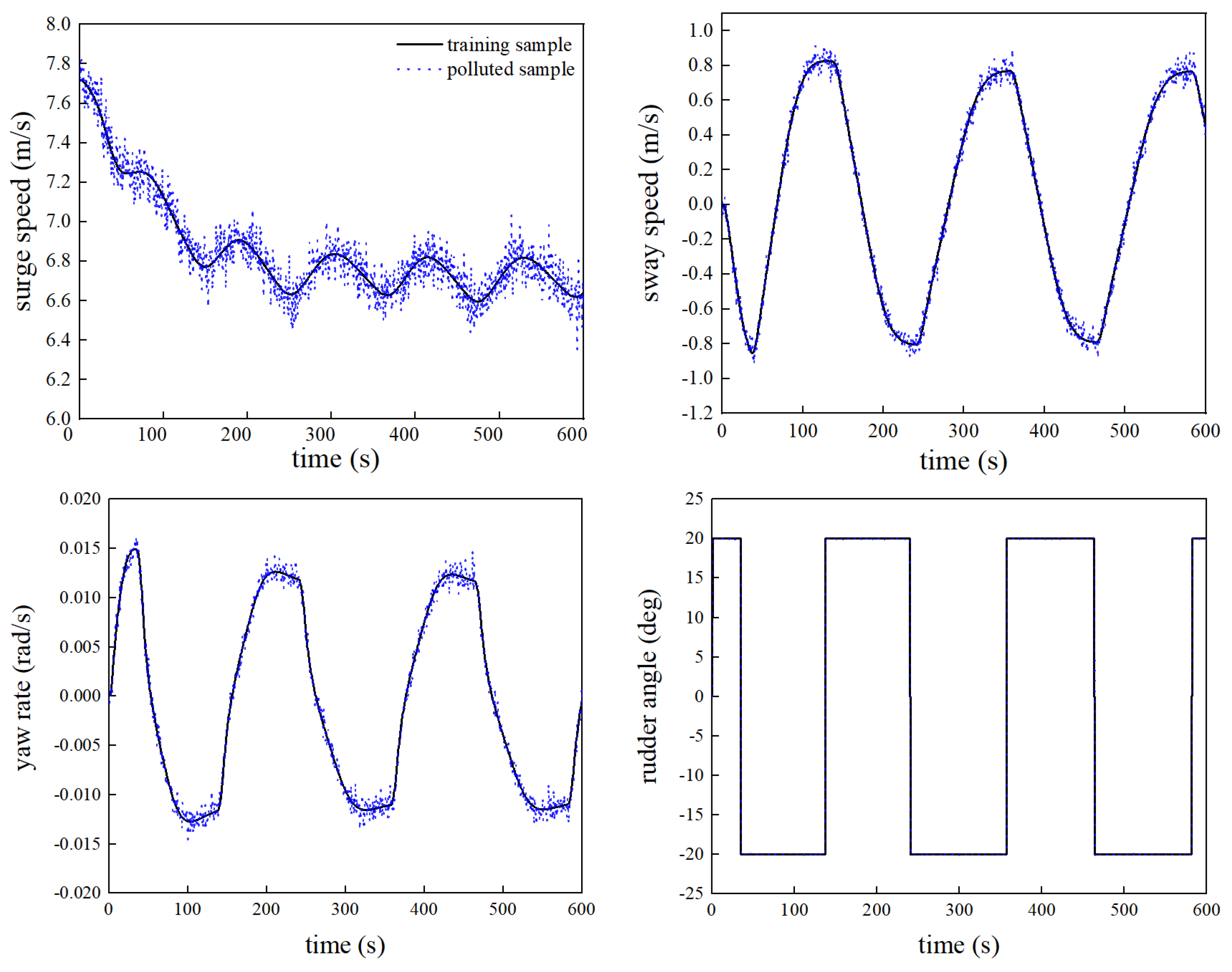
In real marine environmental conditions, ship motion data are collected by onboard sensors. Therefore, the data inevitably contain some level of noise. The training data in this paper are generated from simulations, which do not match the real-world scenario. To validate the robustness of TSVR, Gaussian white noise [29] is added to the training data:
ζ i = ζ i 0 + ζ i m k ζ k 0 ς
where ζ i is the polluted sample. ζ i 0 is the unpolluted sample. ζ i m is the maximum absolute value of ζ i 0 . k ζ is a variable-specified reduction factor ( u 0.2 , δ 0.05 , v ,   r 1 ). ς is Gaussian white noise with a mean of 0 and a variance of 1. In this paper, k 0 = 0.05 corresponds to the training data collected from onboard conventional sensors. Equation (16) introduces measurement noise, corresponding to the fact that the real experimental records are often affected by unknown external disturbances acting on the ship or scaled model [16]. The results of noise addition are shown in Figure 3. TSVR is not a scale-invariant machine learning method [7]. Features of large magnitudes will dominate the input space, thereby reducing prediction accuracy. To avoid this issue, input data need to be normalized [8].
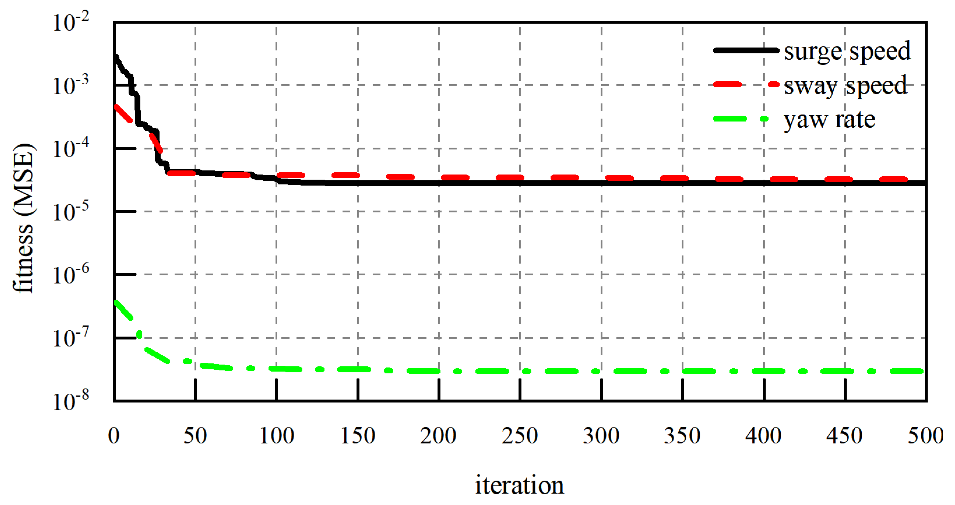
To optimize and adjust the hyperparameters in TSVR, the validation dataset consists of 300 sets of 10°/05° zigzag manoeuvring motion samples. Figure 4 shows the convergence curve of the fitness function. The MSE for the three-DOF approximately converges at the 100th iteration. This indicates that the adjusted hyperparameters are optimal.

4.2. Simulation Results

To validate the effectiveness of TSVR, the testing dataset collected data from four sets of zigzag (Z) manoeuvring motions and two sets of turning circle (TC) manoeuvring motions. Specifically, it includes Z1010, Z1510, Z1515, Z2010, TC20, and TC35. Each dataset contains 1400 sets of samples. Additionally, the SVR model is chosen as a comparative model to validate the effectiveness of TSVR. The same modelling process and modelling data are also used for SVR. To measure the prediction accuracy, the root MSE (RMSE) is selected as the evaluation metric:
R M S E = 1 n t i = 1 n t ( y i y ^ i )
where n t is the number of testing samples. The closer RMSE is to 0, the higher the prediction accuracy of the model.
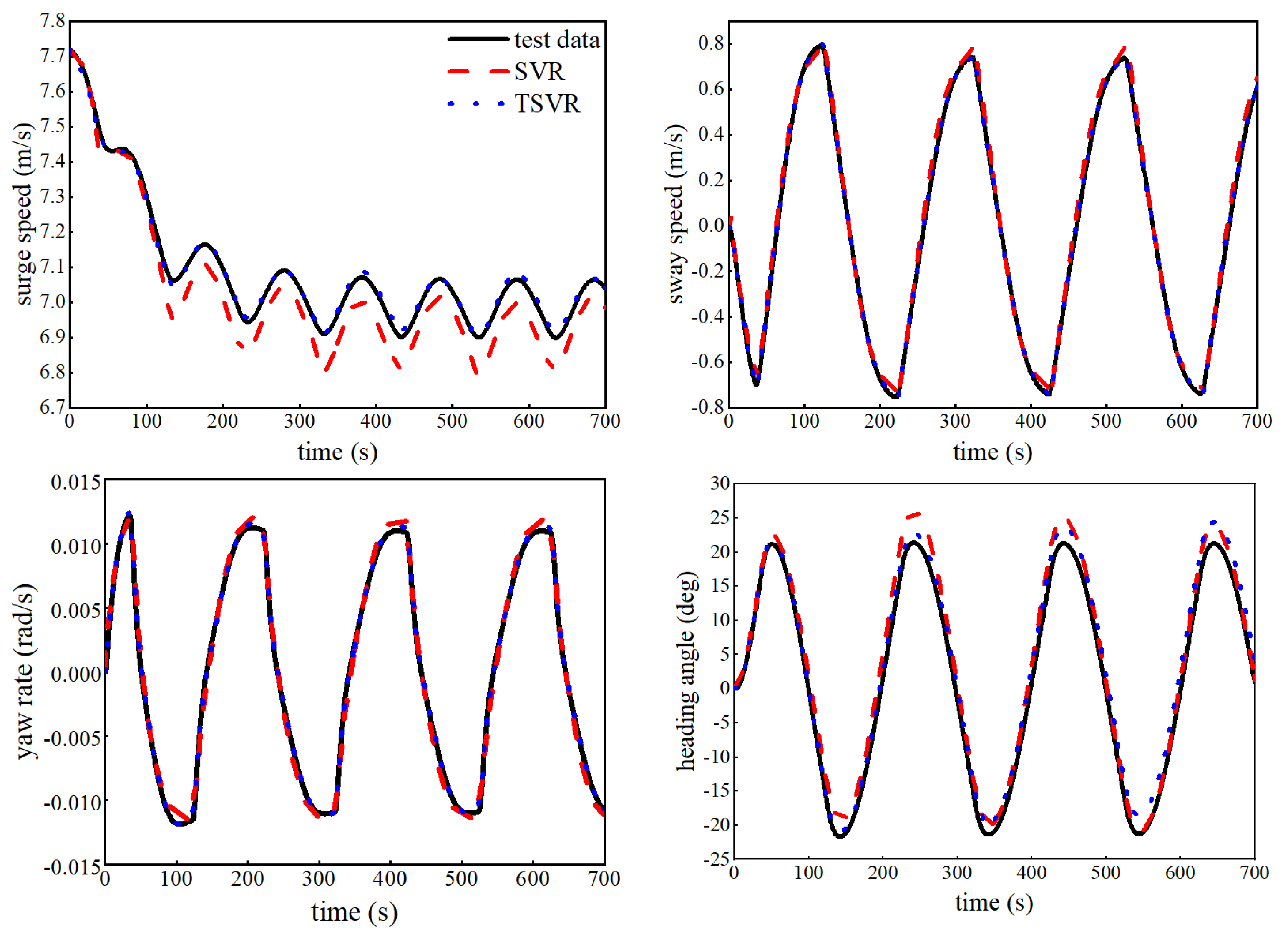
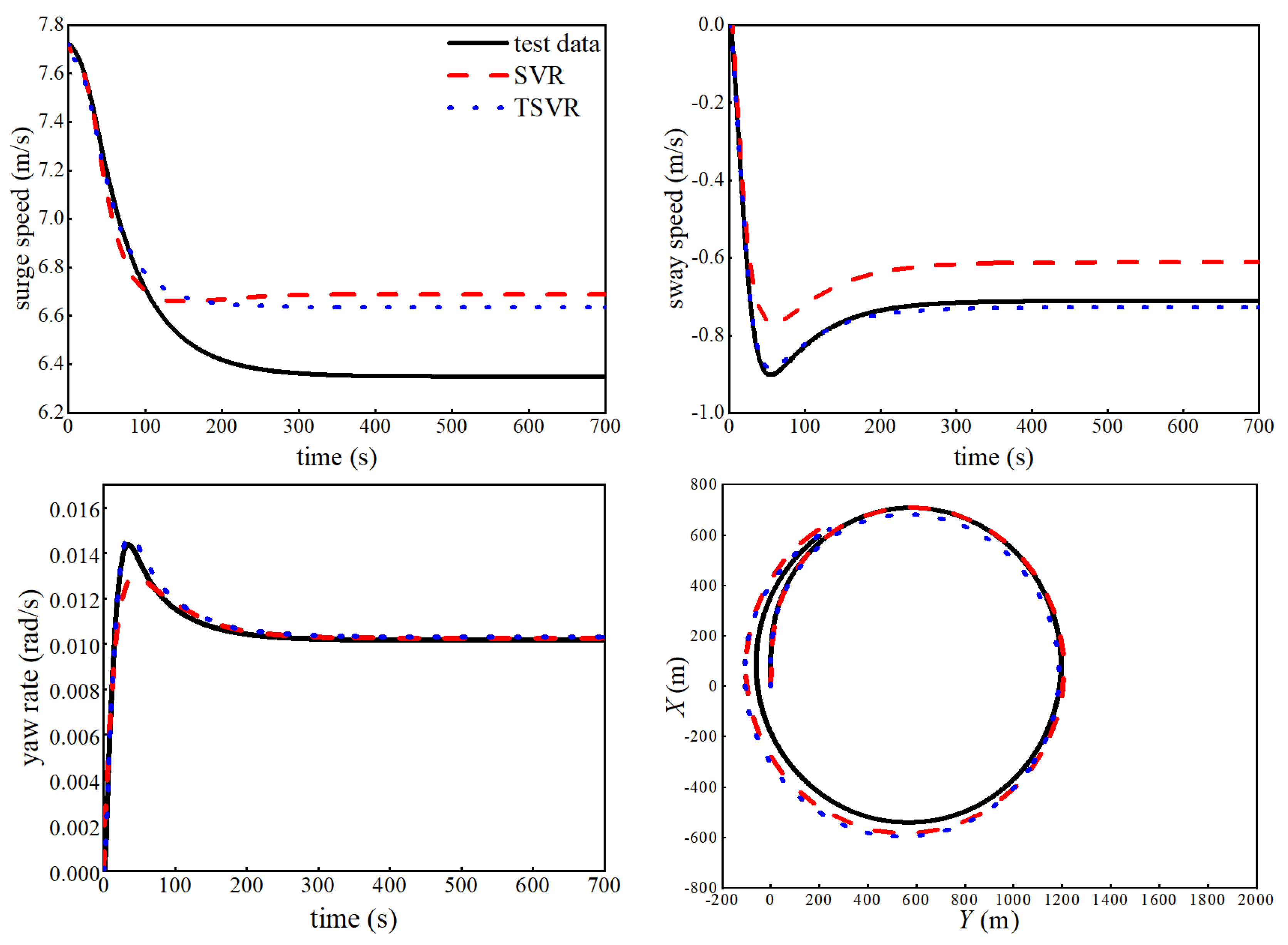
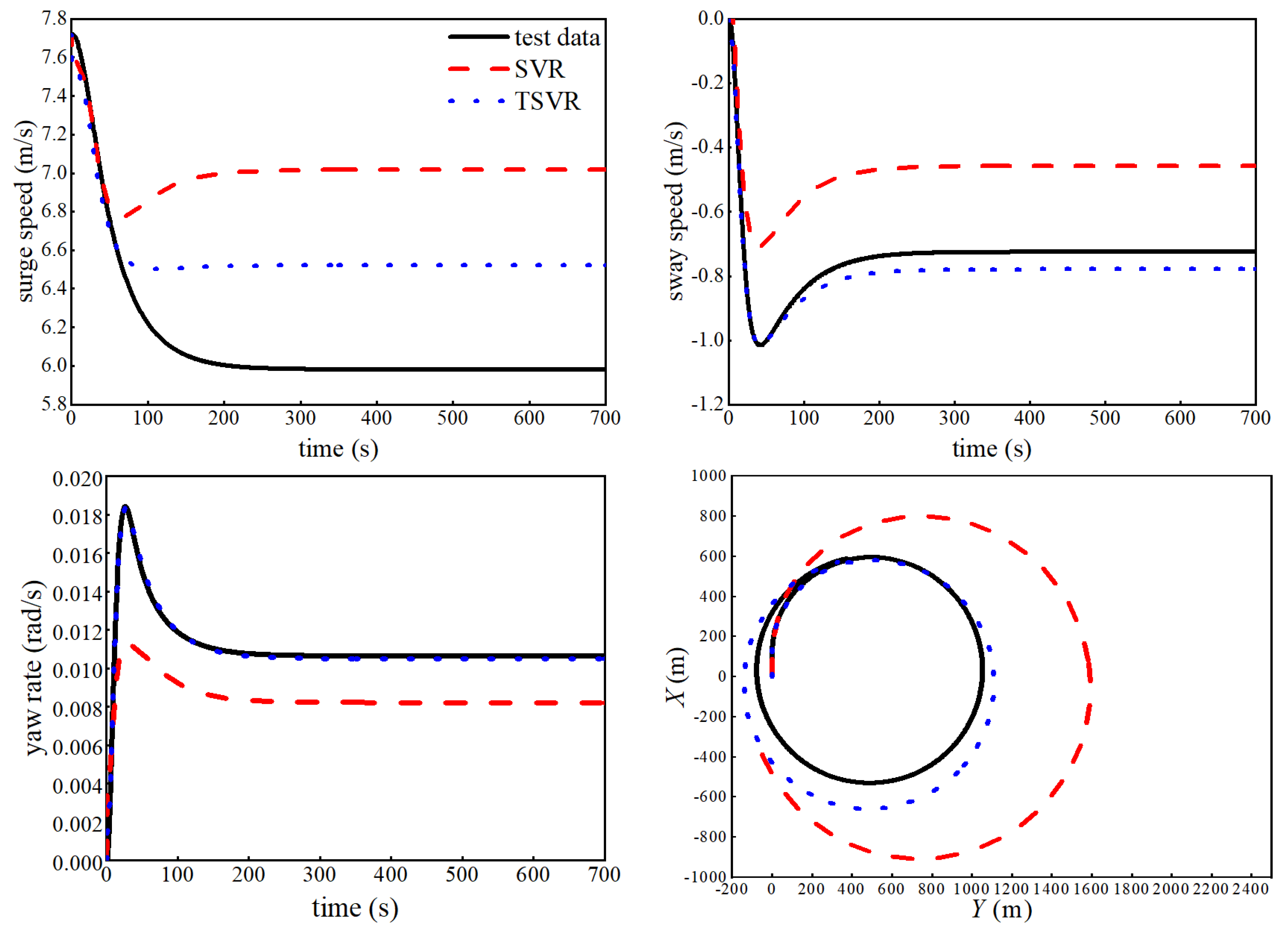
Figure 5 and Figure 6 illustrate the prediction results for Z1010 and Z1515, respectively. The prediction results of SVR exhibit some deviation from the test data, particularly for surge speed and heading angle. In comparison to SVR, the prediction results of TSVR better fit the test data. The robustness of TSVR is demonstrated in accurately predicting under noisy conditions. Turning circle manoeuvring motions contain significantly different dynamic information than zigzag motions. This is because the former involve fixed large rudder angle manoeuvres, while the latter involve frequent rudder angle switching manoeuvres [6]. Therefore, turning circle manoeuvring motions are often used to validate the generalization ability of models trained with Z data [8]. Figure 7 and Figure 8 display the prediction results for TC20 and TC35, respectively. SVR exhibits some deviation in the prediction results for TC20 but remains within an acceptable range. However, as the rudder angle increases, the prediction results for TC35 exhibit significant error. These predictive errors are resulting in considerable trajectory deviation. In contrast to the SVR results, the TSVR results better fit the prediction results to the test data for both TC20 and TC35. The predicted trajectory curve is more consistent with the actual trajectory. This demonstrates the generalizability of TSVR. The better generalization capability of TSVR stems from its utilization of two nonparallel hyperplanes to fit the training data.
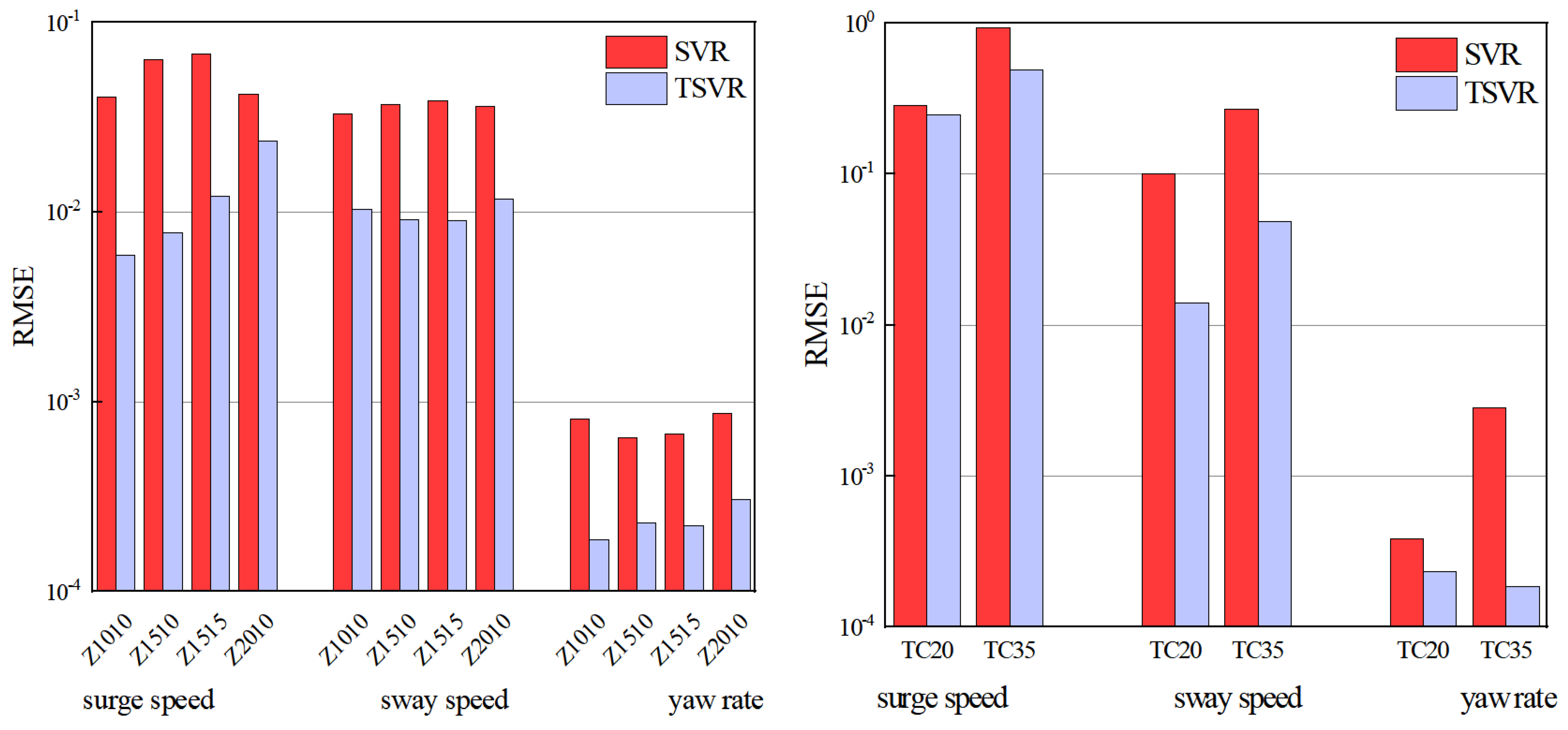
Figure 9 and Figure 10 depict the RMSE and computation time of the prediction results, respectively. It can be observed from the figures that in all tests, TSVR exhibits significantly lower RMSEs than SVR. This indicates that TSVR offers better prediction accuracy. The high accuracy of TSVR not only originates from its inherent excellent performance but also benefits from the PO algorithm. The PO algorithm has found the optimal combination of hyperparameters, maximizing the performance of TSVR. Additionally, both the training and prediction times of TSVR are shorter than those of SVR. This suggests that TSVR has a higher computational efficiency than SVR. The high computational efficiency of TSVR is attributed to its utilization of two small-scale QPPs instead of one large QPP in SVR. Both accuracy and computational efficiency are crucial for the design of ship controllers, as ship controllers must make rapid decisions in complex maritime situations [43]. High accuracy and computational efficiency will ensure the safe navigation of ships at sea.

5. Conclusions

In this study, a novel black-box modelling method named TSVR is proposed for modelling ship dynamics. To enhance the prediction accuracy and computational efficiency of the model, TSVR replaces a large quadratic programming problem (QPP) of SVR with a set of smaller QPPs. The PO algorithm with an optimization objective of MSE is employed to search for the optimal hyperparameters of TSVR. To validate the effectiveness and generalizability of the TSVR model, a three-DOF Mariner class vessel is modelled. Gaussian white noise is introduced into the modelling data to simulate measurement error. The prediction results of zigzag and turning circle manoeuvring motions demonstrate that the TSVR model performs well in terms of prediction accuracy, computational efficiency, robustness, and generalizability.
In this study, TSVR is employed to establish a nonparametric model of ship dynamics. However, the application of TSVRs in the design of controllers has not been explored. Therefore, exploring the performance of TSVRs in controllers will be the focus of future research.

Author Contributions

Conceptualization, L.J., Z.Z. and X.S.; Formal analysis, L.J.; Investigation, L.J.; Methodology, L.J., X.S. and W.W.; Project administration, Z.Z.; Software, L.J.; Writing—original draft, L.J.; Writing—review and editing, L.L. All authors have read and agreed to the published version of the manuscript.

Funding

This work is financially supported by the National Natural Science Foundation of China [grant number: 62303129]; and the Natural Science Foundation of Heilongjiang Province of China [grant number: LH2023F022].

Institutional Review Board Statement

Not applicable.

Informed Consent Statement

Not applicable.

Data Availability Statement

The measured data presented in this study are available from the corresponding author on request.

Conflicts of Interest

The authors declare no conflicts of interest.

References

  1. Zhu, M.; Tian, K.; Wen, Y.Q.; Cao, J.N.; Huang, L. Improved PER-DDPG based nonparametric modeling of ship dynamics with uncertainty. Ocean Eng. 2023, 286, 115513. [Google Scholar] [CrossRef]
  2. Xue, Y.F.; Chen, G.; Li, Z.T.; Xue, G.; Wang, W.; Liu, Y. Online identification of a ship maneuvering model using a fast noisy input Gaussian process. Ocean Eng. 2022, 250, 110704. [Google Scholar] [CrossRef]
  3. Zhu, M.; Hahn, A.; Wen, Y.Q.; Sun, W.Q. Optimized support vector regression algorithm-based modeling of ship dynamics. Ocean Eng. 2019, 90, 101842. [Google Scholar] [CrossRef]
  4. Luo, W.L.; Guedes Soares, C.; Zou, Z.J. Parameter identification of ship maneuvering model based on support vector machines and particle swarm optimization. J. Offshore Mech. Arct. 2016, 138, 031101. [Google Scholar] [CrossRef]
  5. Fossen, T.I. Handbook of Marine Craft Hydrodynamics and Motion Control; John Wiley & Sons: Hoboken, NJ, USA, 2011. [Google Scholar]
  6. Ouyang, Z.L.; Zou, Z.J. Nonparametric modeling of ship maneuvering motion based on Gaussian process regression optimized by genetic algorithm. Ocean Eng. 2021, 238, 109699. [Google Scholar] [CrossRef]
  7. Wang, Z.; Xu, H.; Xia, L.; Zou, Z.; Soares, C.G. Kernel-based support vector regression for nonparametric modeling of ship maneuvering motion. Ocean Eng. 2020, 216, 107994. [Google Scholar] [CrossRef]
  8. Jiang, L.C.; Shang, X.B.; Qi, X.Y.; Ouyang, Z.L.; Zhang, Z. Adaptive ensemble of multi-kernel Gaussian process regressions based on heuristic model screening for nonparametric modeling of ship maneuvering motion. J. Offshore Mech. Arct. Eng. 2025, 147, 011204. [Google Scholar] [CrossRef]
  9. Wu, T.; Li, R.; Chen, Q.; Pi, G.; Wan, S.; Liu, Q. A numerical study on modeling ship maneuvering performance using twin azimuth thrusters. J. Mar. Sci. Eng. 2023, 11, 2167. [Google Scholar] [CrossRef]
  10. Zhang, Z.; Ren, J. Locally weighted non-parametric modeling of ship maneuvering motion based on sparse Gaussian process. J. Mar. Sci. Eng. 2021, 9, 606. [Google Scholar] [CrossRef]
  11. Zhang, X.; Meng, Y.; Liu, Z.; Zhu, J. Modified grey wolf optimizer-based support vector regression for ship maneuvering identification with full-scale trial. J. Mar. Sci. Tech. 2022, 27, 576–588. [Google Scholar] [CrossRef]
  12. Luo, W.; Li, X. Measures to diminish the parameter drift in the modeling of ship manoeuvring using system identification. Appl. Ocean Res. 2017, 67, 9–20. [Google Scholar] [CrossRef]
  13. Liu, A.; Xue, Y.F.; Qin, H.D.; Zhu, Z.B. Physics-informed identification of marine vehicle dynamics using hydrodynamic dictionary library-inspired adaptive regression. Ocean Eng. 2024, 296, 117013. [Google Scholar] [CrossRef]
  14. Zhu, M.; Hahn, A.; Wen, Y.Q.; Bolles, A. Identification-based simplified model of large container ships using support vector machines and artificial bee colony algorithm. Appl. Ocean Res. 2017, 68, 249–261. [Google Scholar] [CrossRef]
  15. Chen, L.; Yang, P.; Li, S.; Tian, Y.; Liu, G.; Hao, G. Grey-box identification modeling of ship maneuvering motion based on LS-SVM. Ocean Eng. 2022, 266, 112957. [Google Scholar] [CrossRef]
  16. Sutulo, S.; Guedes Soares, C. An algorithm for offline identification of ship manoeuvring mathematical models from free-running tests. Ocean Eng. 2014, 79, 10–25. [Google Scholar] [CrossRef]
  17. Sajedi, Y.; Bozorg, M. Robust estimation of hydrodynamic coefficients of an AUV using Kalman and H∞ filters. Ocean Eng. 2019, 182, 386–394. [Google Scholar] [CrossRef]
  18. Perera, L.P.; Oliveira, P.; Guedes Soares, C. System identification of vessel steering with unstructured uncertainties by persistent excitation maneuvers. IEEE J. Ocean. Eng. 2015, 41, 515–528. [Google Scholar] [CrossRef]
  19. Padilla, A.; Yuz, J.L.; Herzer, B. Continuous-time system identification of the steering dynamics of a ship on a river. Int. J. Control 2014, 87, 1387–1405. [Google Scholar] [CrossRef]
  20. Muske, K.R.; Ashrafiuon, H.; Haas, G.; McCloskey, R.; Flynn, T. Identification of a control oriented nonlinear dynamic USV model. In Proceedings of the 2008 American Control Conference, Seattle, WA, USA, 11–13 June 2008; pp. 1–12. [Google Scholar]
  21. Haro Casado, M.; Ferreiro, R.; Velasco, F.J. Identification of nonlinear ship model parameters based on the turning circle test. J. Ship. Res. 2007, 51, 174–181. [Google Scholar] [CrossRef]
  22. Lbrahim, R.A.; Grace, I.M. Modeling of ship roll dynamics and its coupling with heave and pitch. Math. Probl. Eng. 2010, 2010, 934714. [Google Scholar]
  23. Phairoh, T.; Huang, J.K. Adaptive ship roll mitigation by using a U-tube tank. Ocean Eng. 2007, 34, 403–415. [Google Scholar] [CrossRef]
  24. Jiang, L.C.; Shang, X.B.; Jin, B.; Zhang, Z.; Zhang, W. Black-box modeling of ship maneuvering motion using multi-output least-squares support vector regression based on optimal mixed kernel function. Ocean Eng. 2024, 293, 116663. [Google Scholar] [CrossRef]
  25. Lewis, E.V. Principles of Naval Architecture Second Revision; SNAME: London, UK, 1988. [Google Scholar]
  26. Yasukawa, H.; Yoshimura, Y. Introduction of MMG standard method for ship maneuvering predictions. J. Mar. Sci. Technol. 2015, 20, 37–52. [Google Scholar] [CrossRef]
  27. Johan Åström, K. Design of fixed gain and adaptive ship steering autopilots based on the Nomoto model. In Proceedings of the Symposium on Ship Steering Automatic Control, Genoa, Italy, 15 January 1980. [Google Scholar]
  28. Luo, W.; Cong, H. Control for ship course-keeping using optimized support vector machines. Algorithms 2016, 9, 52. [Google Scholar] [CrossRef]
  29. Zhang, Y.Y.; Wang, Z.H.; Zou, Z.J. Black-box modeling of ship maneuvering motion based on multi-output nu-support vector regression with random excitation signal. Ocean Eng. 2022, 257, 111279. [Google Scholar] [CrossRef]
  30. Wang, Z.; Kim, J.; Im, N. Non-parameterized ship maneuvering model of Deep Neural Networks based on real voyage data-driven. Ocean Eng. 2023, 284, 115162. [Google Scholar] [CrossRef]
  31. Moreno, R.; Moreno-Salinas, D.; Aranda, J. Black-box marine vehicle identification with regression techniques for random manoeuvres. Electronics 2019, 8, 492. [Google Scholar] [CrossRef]
  32. Moreno-Sallnas, D.; Moreno, R.; Pereira, A.; Aranda, J.; de la Cruz, J.M. Modelling of a surface marine vehicle with kernel ridge regression confidence machine. Appl. Soft Comput. 2019, 76, 237–250. [Google Scholar] [CrossRef]
  33. Skulstad, R.; Li, G.; Fossen, T.I.; Vik, B.; Zhang, H. A hybrid approach to motion prediction for ship docking-integration of a neural network model into the ship dynamic model. IEEE Trans. Instrum. Meas. 2021, 70, 2501311. [Google Scholar] [CrossRef]
  34. Diez, M.; Serani, A.; Campana, E.F.; Stern, F. Time-series forecasting of ships maneuvering in waves via dynamic mode decomposition. J. Ocean Eng. Mar. Energy 2022, 8, 471–478. [Google Scholar] [CrossRef]
  35. Xue, Y.; Liu, Y.; Xue, G.; Chen, G. Identification and prediction of ship maneuvering motion based on a Gaussian process with uncertainty propagation. J. Mar. Sci. Eng. 2021, 9, 804. [Google Scholar] [CrossRef]
  36. Luo, W.; Moreira, L.; Guedes Soares, C. Manoeuvring simulation of catamaran by using implicit models based on support vector machines. Ocean Eng. 2014, 82, 150–159. [Google Scholar] [CrossRef]
  37. Ouyang, Z.L.; Zou, Z.J.; Zou, L. Nonparametric modeling and control of ship steering motion based on local Gaussian process regression. J. Mar. Sci. Eng. 2023, 11, 2161. [Google Scholar] [CrossRef]
  38. Liu, S.-Y.; Ouyang, Z.-L.; Chen, G.; Zhou, X.; Zou, Z.-J. Black-box modeling of ship maneuvering motion based on Gaussian process regression with wavelet threshold denoising. Ocean Eng. 2023, 271, 113765. [Google Scholar] [CrossRef]
  39. Shuai, Y.H.; Li, G.Y.; Cheng, X.; Skulstad, R.; Xu, J.; Liu, H.; Zhang, H. An efficient neural-network based approach to automatic ship docking. Ocean Eng. 2019, 191, 106514. [Google Scholar] [CrossRef]
  40. Vapnik, V.N. An overview of statistical learning theory. IEEE Trans. Neural Netw. 1999, 10, 988–999. [Google Scholar] [CrossRef]
  41. Gu, B.; Fang, J.; Pan, F.; Bai, Z. Fast clustering-based weighted twin support vector regression. Soft Comput. 2020, 24, 6101–6117. [Google Scholar] [CrossRef]
  42. Platt, J. Fast Training of Support Vector Machines Using Sequential Minimal Optimization; MIT Press: Cambridge, MA, USA, 2000. [Google Scholar]
  43. Xu, P.L.; Qin, H.D.; Ma, J.G.; Deng, Z.C.; Xue, Y.F. Data-driven model predictive control for ships with Gaussian process. Ocean Eng. 2023, 268, 113420. [Google Scholar] [CrossRef]
  44. Peng, X. TSVR: An efficient twin support vector machine for regression. Neural Netw. 2010, 23, 365–372. [Google Scholar] [CrossRef]
  45. Xu, Y.; Wang, L. A weighted twin support vector regression. Knowl.-Based Syst. 2012, 33, 92–101. [Google Scholar] [CrossRef]
  46. Tanveer, M.; Shubham, K.; Aldhaifallah, M.; Ho, S. An efficient regularized K-nearest neighbor based weighted twin support vector regression. Knowl.-Based Syst. 2016, 94, 70–87. [Google Scholar] [CrossRef]
  47. Houssein, E.H. Particle swarm optimization-enhanced twin support vector regression for wind speed forecasting. J. Intell. Syst. 2019, 28, 905–914. [Google Scholar] [CrossRef]
  48. Cheng, H.X.; Huang, Z.; Luo, X.L. PH Prediction desulfurization system in thermal power plant based on improved twin support vector machine. J. Qingdao Univ. Sci. Technol. 2019, 40, 101–106. [Google Scholar]
  49. Gómez, D.; Salvador, P.; Sanz, J.; Casanova, J.L. Potato yield prediction using machine learning techniques and sentinel 2 data. Remote Sens. 2019, 11, 1745. [Google Scholar] [CrossRef]
  50. Gupta, D.; Pratama, M.; Ma, Z.; Li, J.; Prasad, M. Financial time series forecasting using twin support vector regression. PLoS ONE 2019, 14, e0211402. [Google Scholar] [CrossRef] [PubMed]
  51. Wu, Q.; Zhang, H.Y. Feature selection based on twin support vector regression. In Proceedings of the 2019 IEEE Symposium Series on Computational Intelligence (SSCI), Xiamen, China, 6–9 December 2019. [Google Scholar]
  52. Abdollahzadeh, B.; Khodadadi, N.; Barshandeh, S.; Trojovský, P.; Gharehchopogh, F.S.; El-Kenawy, E.-S.M.; Abualigah, L.; Mirjalili, S. Puma optimizer (PO): A novel metaheuristic optimization algorithm and its application in machine learning. Cluster Comput. 2024. [Google Scholar] [CrossRef]
  53. Chislett, M.S.; Strøm-Tejsen, J. Planar Motion Mechanism Tests and Full-Scale Steering and Maneuvering Predictions for a Mariner Class Vessel; Technical Report Hy-6. Hydro- and Aerodynamics Laboratory: Lyngby, Denmark, 1965. [Google Scholar]
  54. Wang, Z.H.; Zou, Z.J.; Guedes Soares, C. Identification of ship manoeuvring motion based on nu-support vector machine. Ocean Eng. 2019, 183, 270–281. [Google Scholar] [CrossRef]
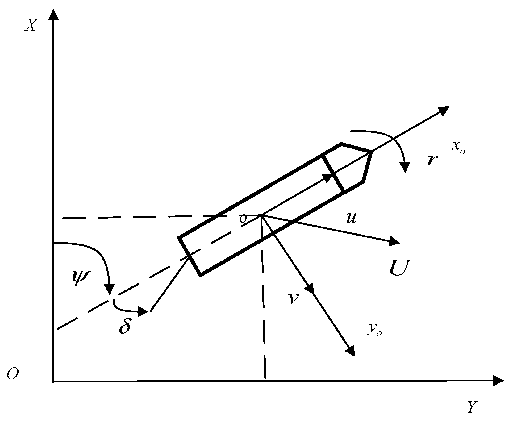
Figure 1. Ship coordinate systems.
Jmse 12 00754 g001
Figure 2. Nonparametric modelling process for ship dynamics. Light orange, blue, and dark orange in the figure represent the training, validation, and testing processes, respectively.
Jmse 12 00754 g002
Figure 3. Polluted training data.
Jmse 12 00754 g003
Figure 4. Convergence curves for hyperparameters optimization.
Jmse 12 00754 g004
Figure 5. Prediction results for Z1010.
Jmse 12 00754 g005
Figure 6. Prediction results for Z1515.
Jmse 12 00754 g006
Figure 7. Prediction results for TC20.
Jmse 12 00754 g007
Figure 8. Prediction results for TC35.
Jmse 12 00754 g008
Figure 9. Prediction accuracy (RMSE).
Jmse 12 00754 g009
Figure 10. Computation times.
Jmse 12 00754 g010
Table 1. Main particulars of the Mariner class vessel.
ParticularsUnitValue
Length overallm171.8
Length between perpendicularsm160.93
Design waterline lengthm158.72
Maximum beamm23.17
Design draftm8.23
Design displacementm318,541
Number of propellers--1
Number of blades--4
Propeller diameterm6.706
Propeller pitch ratio--0.964
Developed area ratio--0.565
Disclaimer/Publisher’s Note: The statements, opinions and data contained in all publications are solely those of the individual author(s) and contributor(s) and not of MDPI and/or the editor(s). MDPI and/or the editor(s) disclaim responsibility for any injury to people or property resulting from any ideas, methods, instructions or products referred to in the content.