Ship Flow of the Ryuko-maru Calculated by the Reynolds Stress Model Using the Roughness Function at the Full Scale

Abstract

The k-omega SST turbulence model is extensively employed in Reynolds-averaged Navier–Stokes (RANS)-based Computational Fluid Dynamics (CFD) calculations. However, the accuracy of the estimation of viscous resistance and companion flow distribution for full-sized vessels is not sufficient. This study conducted a computational analysis of the flow around the Ryuko-maru at model-scale and full-scale Reynolds numbers utilizing the Reynolds stress turbulence model (RSM). The obtained Reynolds stress distribution from the model-scale computation was compared against experimental measurements to assess the capability of the RSM. Furthermore, full-scale computations were performed, incorporating the influence of hull surface roughness, with the resulting wake distributions juxtaposed with the actual ship measurements. The full-scale calculation employed the sand-grain roughness function, and an optimal roughness length scale was determined by aligning the computed wake distribution with Ryuko-maru’s measured data. The results of this study will allow for the direct performance estimation of full-scale ships and contribute to the design technology of performance.

1. Introduction

In response to the pressing environmental challenge of global warming, the International Maritime Organization (IMO) has set a target of achieving zero greenhouse gas (GHG) emissions from ships by 2050 [1]. This necessitates adopting alternative fuels and natural energy sources to replace heavy oil as well as developing innovative propulsion systems. Despite alternative energy sources’ inherent lower fuel efficiency, there is an urgent need to accelerate the optimization of ship forms and the advancement of energy-saving devices. Consequently, there is a demand for highly accurate prediction technology to evaluate full-scale ship performance.

While numerous studies have focused on Computational Fluid Dynamics (CFD) calculations for ship flow using model ships to achieve accurate estimates of ship performance, there is a growing preference for direct calculations at full-scale Reynolds numbers. This approach avoids the need to extrapolate from model ship Reynolds numbers to full-scale equivalents. Undertaking full-scale CFD calculations at a practical level underscores the importance of validating the CFD methodology by comparing the results with empirical measurement data.

Many CFD analyses have been conducted to predict ship flow, with Pena et al. [2] providing a comprehensive review of turbulence models’ efficacy in estimating ship performance. Reynolds-averaged Navier–Stokes (RANS)-based computational methods are widely used, employing two-equation turbulence models like the k–ε or k-omega SST. However, these models exhibit limitations in accurately estimating viscous resistance. Matsuda et al. [3] conducted a comparative study of ship flow calculations using the k-omega SST (a two-equation model) and the Reynolds stress turbulence model (RSM) (a seven-equation model) at model-scale Reynolds numbers across various hull forms. While the k-omega SST is adequate in estimating form factor K and wake distribution for slender ships, it underestimates form factor K, resulting in a smaller stern longitudinal vortex size at the propeller plane compared to experimental results for full-sized vessels. Matsuda et al. demonstrated that the RSM offers more accurate estimates for form factor and wake distribution, particularly for bulk carriers and oil tankers.

Pena et al. [2] highlighted various applications of CFD at full-scale Reynolds numbers [4,5,6], citing studies by Song et al. [7] and Pena et al. [8], which examined KCS and KVLCC2 flows at both model- and full-scale Reynolds numbers, accounting for hull surface roughness using wall function boundary conditions. Hull surface roughness significantly increases frictional and viscous drag, wave pattern, and wake distribution. Pena et al. [8] conducted full-scale calculations for a general cargo ship (Regal), analyzing the hull’s detailed flow field and discussing velocity, shear pressure, and vorticity distribution. Ohashi [9] calculated the flow around the Ryuko-maru (an older model VLCC) at full-scale Reynolds numbers, accounting for surface roughness through wall-resolved and wall function boundary conditions. These calculations were compared to measured wake distributions obtained from actual ship measurements. The comparison revealed that when roughness effects were considered, the wake distribution obtained from CFD calculations demonstrated improved agreement with the full-scale measured results compared to those assuming a smooth surface. Furthermore, considering uncertainty, the wall function approach was more effective for CFD calculations in full-scale ship scenarios. Sakamoto et al. [10] similarly employed this method for calculations involving bulk carriers and container ships fitted with ducts, mirroring the approach taken by Ohashi [9]. Their findings demonstrated strong agreement in wake flow distribution, even when considering the presence of energy-saving devices. Accurately estimating the additional frictional resistance exerted on painted hull surfaces requires a thorough understanding of the roughness function specific to such surfaces. Many roughness functions employed in CFD calculations are tailored to sand-grain roughness. Consequently, understanding the roughness length scale specific to painted surfaces is crucial for accurate full-scale ship flow calculations. To verify the effectiveness of the RSM in more detail, it is important to evaluate it at the level of Reynolds stress, but there are no previous studies. Few studies have applied the RSM to CFD calculations at the full scale and compared the wake flow distribution with the full-scale test results. Furthermore, there is no standardized method that takes into account the roughness of the hull surface of a full-scale model, and it has not been fully verified how to set the roughness height to perform a reasonable calculation at the full scale.

This study calculated ship flow at the model scale using the RSM for enhanced wake distribution accuracy, validating it against Reynolds stresses from wind tunnel experiments. The influence of hull surface roughness was incorporated using wall function methodology, integrating a sand-grain roughness function, and exploring an appropriate roughness length scale through comparison with empirical wake distribution data. In this study, the effectiveness of the RSM can be confirmed in more detail by comparing the CFD calculation results with the experimental Reynolds stresses. Furthermore, by developing a CFD calculation method that takes into account the surface roughness of the hull, it will be possible to directly estimate the viscous resistance and the wake distribution with high accuracy on a practical number of grids. This will contribute to the improvement in design technology.

2. Comparison of CFD Calculations and Experimental Results of Reynolds Stress at the Model Scale

Prior research has established that the RSM outperforms the k-omega SST, a two-equation model, in predicting form factor K at the model ship scale. This is attributed to its superior accuracy in forecasting wake flow distribution. For a precise estimation of ship flow distribution, it is crucial to assess not only velocity distribution but also Reynolds stresses. However, validating the RSM’s full-scale wake distribution accuracy poses challenges because direct measurements are unavailable. CFD simulations were conducted for the Ryuko-maru at the model ship scale, comparing results from the k-omega SST and the RSM–linear pressure strain correlation model with two layers (LPST) to assess the RSM’s Reynolds stress prediction accuracy. The comparison utilized data from wind tunnel tests performed by Suzuki et al. [11] using a 3 m model ship in the Osaka University research wind tunnel (with measurement section dimensions of L × B ×D = 9.5 m × 1.8 m × 1.8 m). The model ship was suspended in the tunnel’s center using piano wire, with a wind tunnel blockage rate of approximately 6%. Flow field measurements were obtained using a triple-sensor hot-wire system, with data sampling at 10 kHz, acknowledging inherent errors of approximately 5% for time-averaged flow velocity and approximately 10% for Reynolds stress components. Furthermore, a V&V process was conducted to compare the two-equation k-omega SST model with the RSM–LPST.

2.1. Computational Conditions

The RSM was assessed using the hull form of the Ryuko-maru, a 200,000 DWT tanker built in Japan with a Cb value of 0.83. CFD validation data for this vessel, made publicly available by Namimatsu et al. [12], were utilized. The wake distribution of the ship was also measured at the full scale using a five-hole pitot tube. Figure 1 illustrates the 3D model of the Ryuko-maru, while Table 1 provides its principal dimensions.

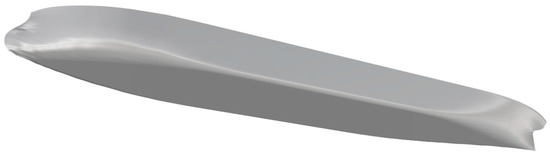
Figure 1. 3D model of Ryuko-maru.

Table 1. Principle dimensions of Ryuko-maru.

Model/Ship	Ship	Model
Lpp (m)	300.00	3.000
B (m)	50.00	0.500
D (m)	25.00	0.250
d (m)	18.86	0.189
Dp (m)	9.20	0.092
α	-	100.00
Cb	0.83

The CFD simulations were conducted using STAR-CCM+ version 16.02. Two turbulence models were employed: k-omega SST and RSM–LPST. The RSM–LPST, based on the LPS (linear pressure strain correlation) model [13] with a wall function developed by Gibson and Launder [14], is specifically designed for low Reynolds numbers, with y ≤ +1 for grid points near the wall surface. It uses a model coefficient for the pressure–strain correlation term reported by Launder and Shima [15]. Previous research by Matsuda et al. [3] demonstrated the effectiveness of LPST for CFD calculations at model ship scales, thus justifying its selection for this study.

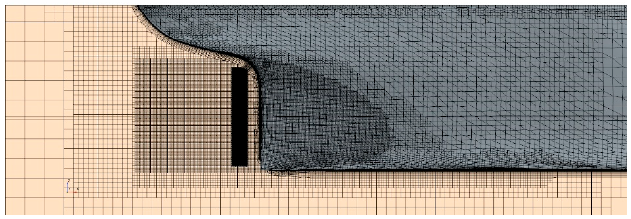
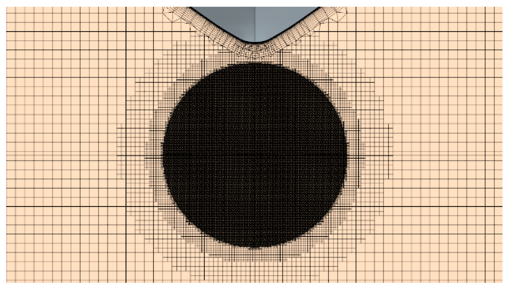
As depicted in Figure 2, the computational domain spans dimensions of 5.0 L_pp × 5.0 L_pp × 0.625 L_pp (both sides), with only the area below the draft considered in the CFD computations. In contrast, wind tunnel tests utilized a double-model setup. A medium grid arrangement, illustrated in Figure 3, shows the surface grid of a 3 m model of the Ryuko-maru. Figure 4 shows the volume grid of the center plane. Figure 5 shows the volume grid in the propeller plane. Dense grids are arranged to adapt to the complex flow around the stern. The first layer of grids on the hull surface was configured to achieve y+ ≈ 1. To ensure accuracy, three grid resolutions (coarse, medium, and fine) were generated for verification purposes, following the methodology employed by Matsuda et al. [3] the simulations were conducted under uniform flow conditions, as detailed in Table 2.

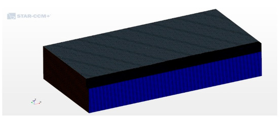
Figure 2. Volume grid of whole area.

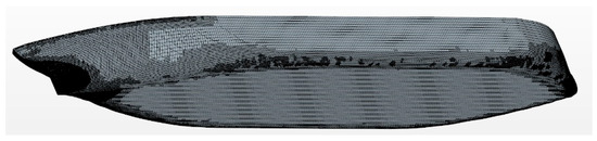
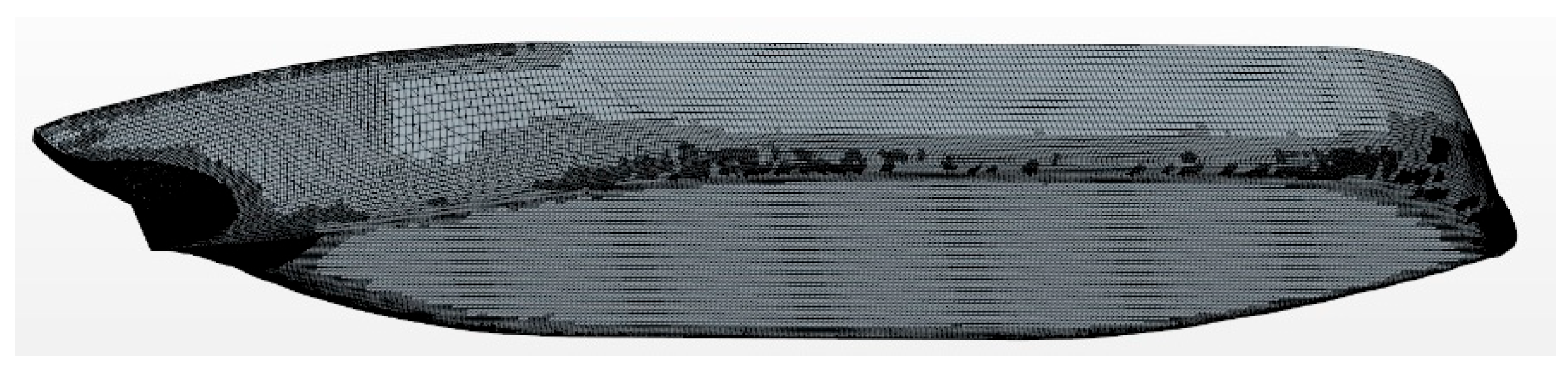
Figure 3. Surface grid of 3 m model of Ryuko-maru.

Figure 4. Volume grid around hull of 3 m model.

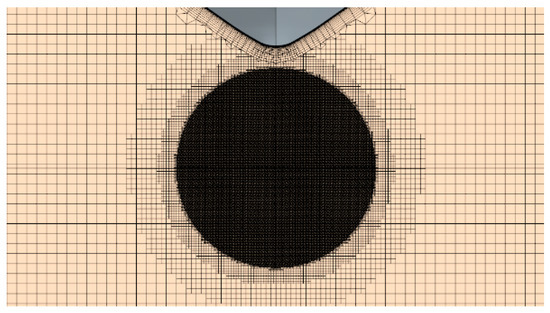
Figure 5. Volume grid of 3 m model in propeller plane.

Table 2. Computational conditions of 3 m model.

Vm (m/s)	20.0
ρ (kg/m3)	1.146
ν × 10−5 (m2/s)	1.6509
Rn × 106	3.63

2.2. Verification Method and Results

The verification used the ITTC method [16]. Table 3 depicts the verification grid generation results. The grid counts were determined to maintain an R_i of approximately 1.4, specifically, approximately 22 million for the fine grid, approximately 8 million for the medium grid, and approximately 3 million for the coarse grid.

Table 3. Results of grid refinement ratio $r_i$ of 3 m model.

Fine	NC1	22,101,990
Midium	NC3	8,006,215
Coarse	NC4	2,933,781
	Ri	1.400
	Ri,21	1.403
	Ri,32	1.397

The results of the CFD calculations are presented in Table 4. The verification results for ${\epsilon }_{21}$, ${\epsilon }_{32}$, $R$, $U_i,$ and $U_{SN}$ are shown in Table 5.

Table 4. Results of CFD calculation of 3 m model.

No.	Turbulance Model	Grid	Fall (N)	Fvis (N)	CT × 103	Cf × 103
1	k-ω SST	Coarse	2.00	1.60	3.783	3.012
2		Midium	2.07	1.61	3.900	3.048
3		Fine	2.01	1.60	3.796	3.012
4	LPST	Coarse	2.17	1.74	4.091	3.289
5		Midium	2.26	1.81	4.275	3.409
6		Fine	2.18	1.74	4.108	3.285

Table 5. Results of verification of 3 m model.

	${\mathit{\epsilon }}_{21}$	${\mathit{\epsilon }}_{32}$	$\mathit{R}$	${\mathit{\epsilon }}_{\mathit{i},32}$$/{\mathit{\epsilon }}_{\mathit{i},21}$	${\mathit{U}}_{\mathit{i}}$	${\mathit{U}}_{\mathit{S}\mathit{N}}$ (%CTfine)
k-ω SST	0.1035	−0.1172	−0.8832	−1.1323	0.059	1.54%
LPS	0.1662	−0.1835	−0.9058	−1.1040	0.092	2.23%

The k-omega SST and the LPST on the three grids performed in this study are not in the direction of convergence as the grids are made finer. This may be due to the fact that even a coarse grid is generally sufficient. In addition, the LPST estimated a larger overall viscous resistance to the k-omega SST. This result follows the same trend as that of Matsuda et al. [3]. The calculated numerical uncertainty $U_{SN}$ (1.54%) of the k-omega SST model is lower than that of the RSM–LPS $U_{SN}$ (2.23%). However, the $U_{SN}$ for both is sufficiently small, and the variation in hydrodynamic forces is also small enough in the three grids. Consequently, a detailed comparison of wake distributions was conducted for the medium grid.

2.3. Results of CFD Calculation of Reynolds Stress

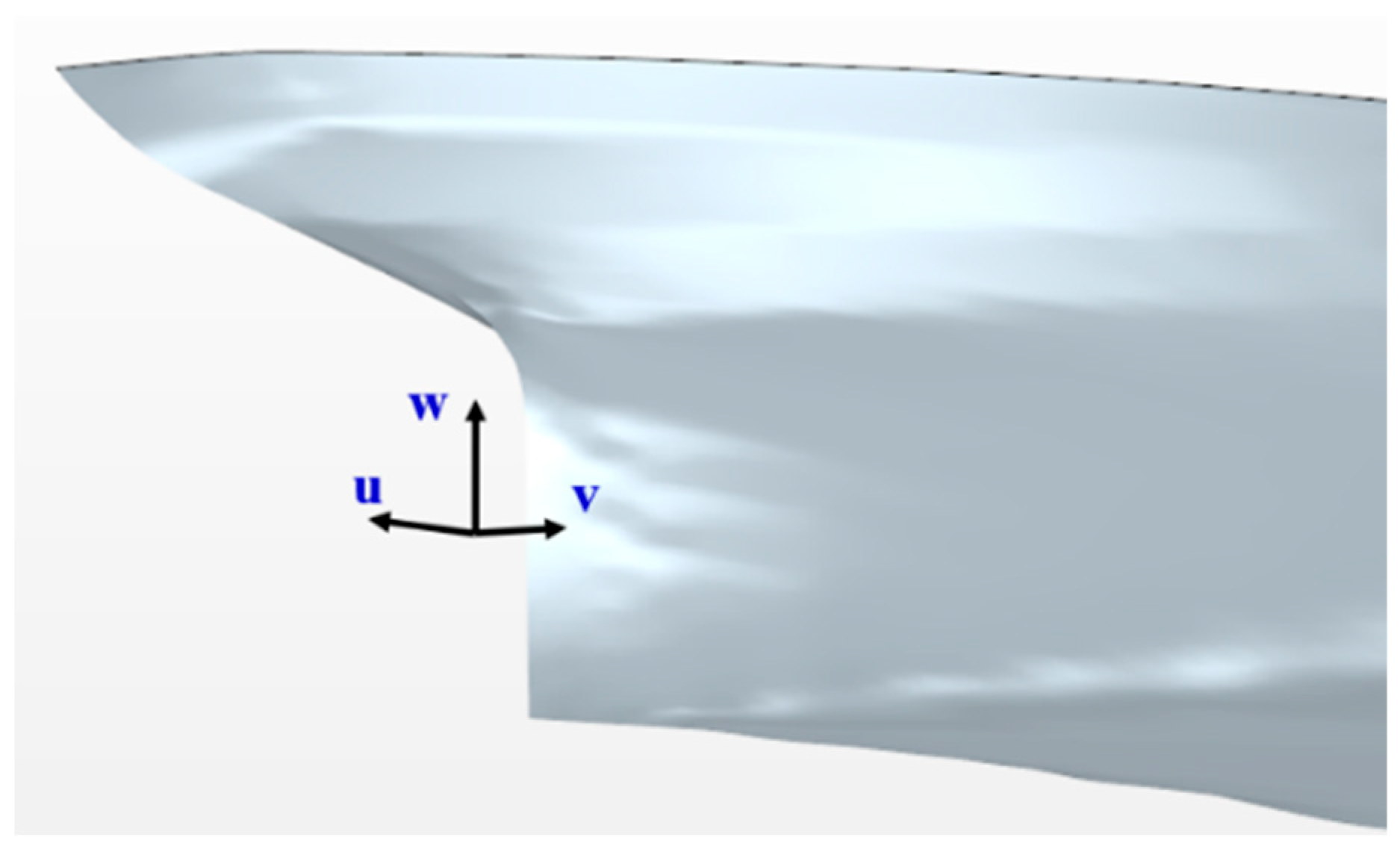
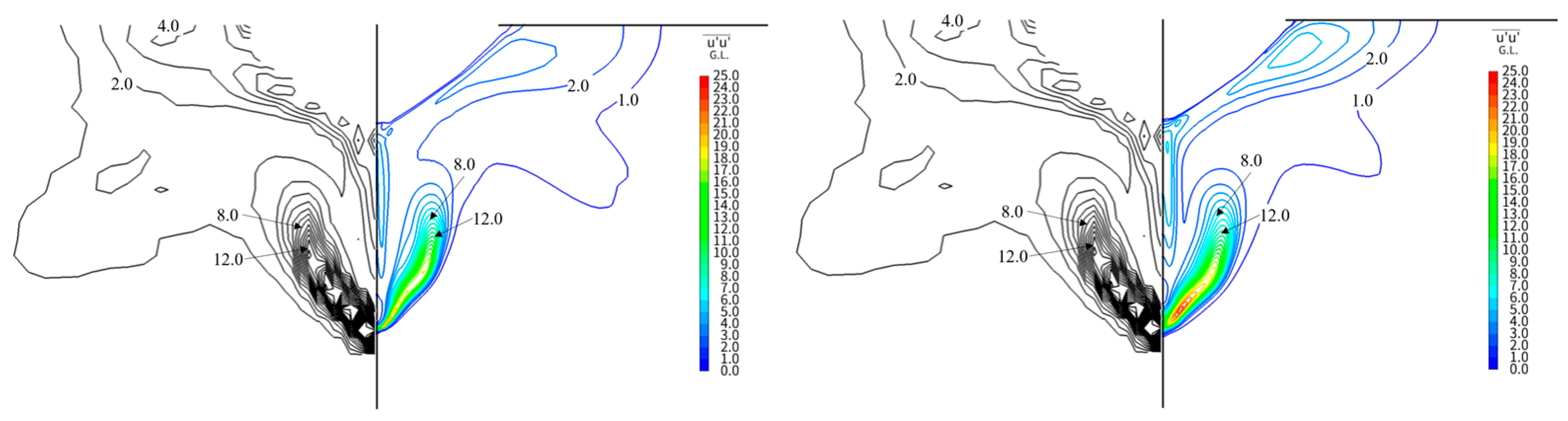
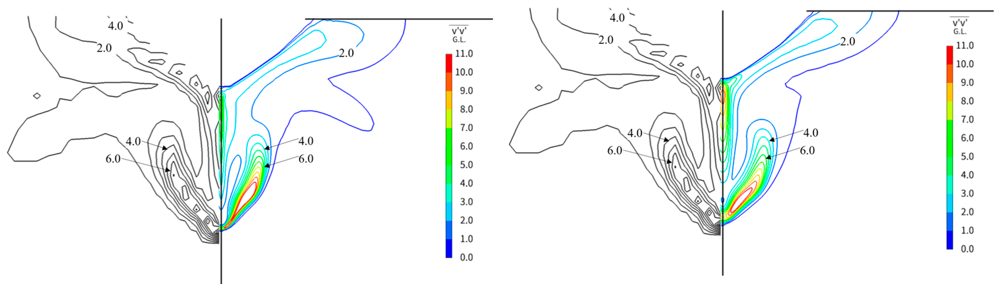
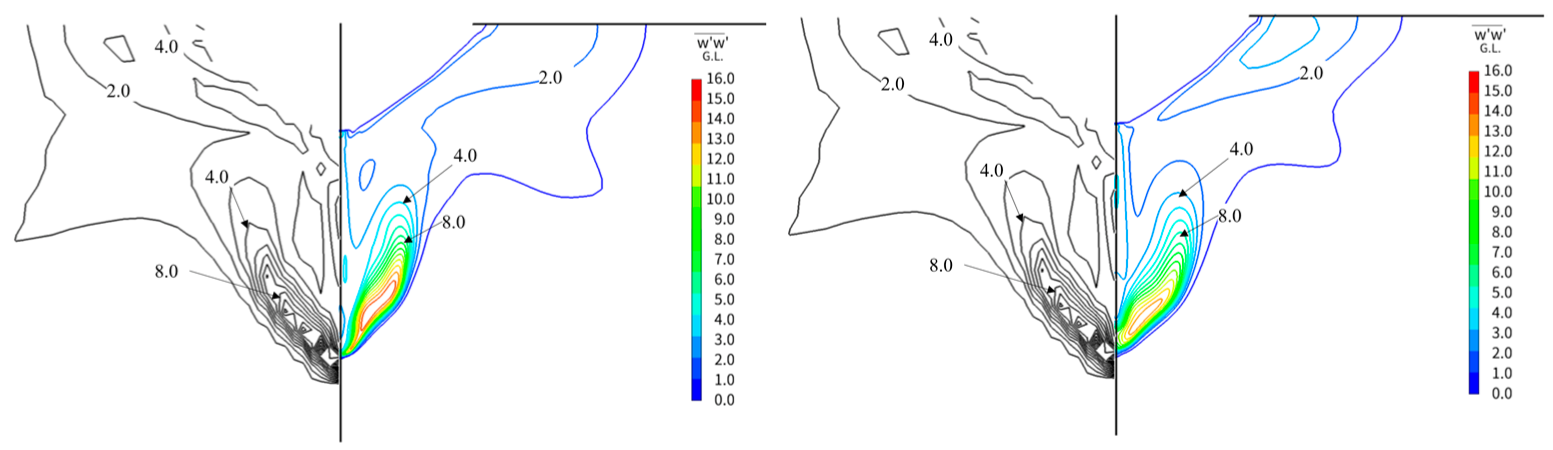
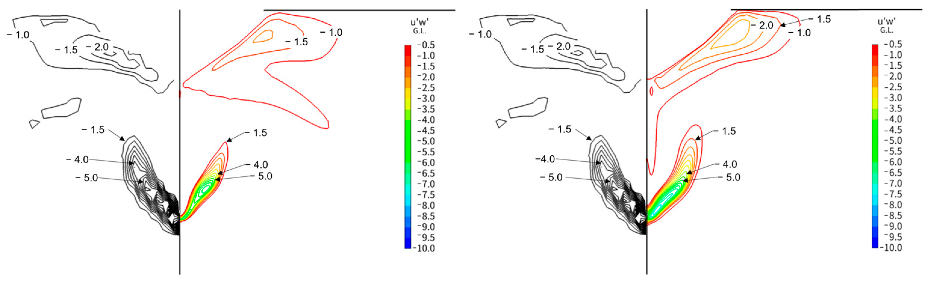
The definition of flow direction is shown in Figure 6. The distribution of the contour plot of Vx/V0 is shown in Figure 7, $V_{cf}$/V0 in Figure 8, $\overline{u^{\prime }{u}^{\prime }}$ in Figure 9, $\overline{v^{\prime }{v}^{\prime }}$ in Figure 10, $\overline{w^{\prime }{w}^{\prime }}$ in Figure 11, $\overline{u^{\prime }{w}^{\prime }}$ in Figure 12, and turbulence kinetic energy k in Figure 13. Figure 7, Figure 8, Figure 9, Figure 10, Figure 11, Figure 12 and Figure 13 shows the wind tunnel test results on the left and the CFD calculation results on the right. Vx is the longitudinal velocity (m/s) and V0 is the ship speed (m/s). $\overline{u^{\prime }{u}^{\prime }}$, $\overline{v^{\prime }{v}^{\prime }}$, $\overline{w^{\prime }{w}^{\prime }}$, and $\overline{u^{\prime }{w}^{\prime }}$ are the Reynolds stresses of u, v, w, and uw. $\overline{u^{\prime }{u}^{\prime }}$, $\overline{v^{\prime }{v}^{\prime }}$, $\overline{w^{\prime }{w}^{\prime }}$, $\overline{u^{\prime }{w}^{\prime }}$, and k are nondimensionalized at V0². The crossflow velocity magnitude is defined as follows:

$$V_{cf}=\sqrt{V_y^2+V_z^2}$$

(1)

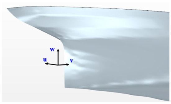
Figure 6. Crossflow distribution of SPIV (left) and CFD (right) at 110 mm from A.P.

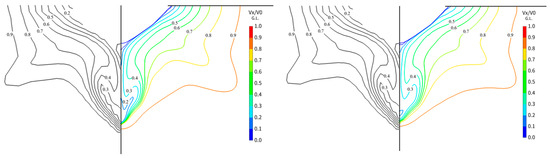
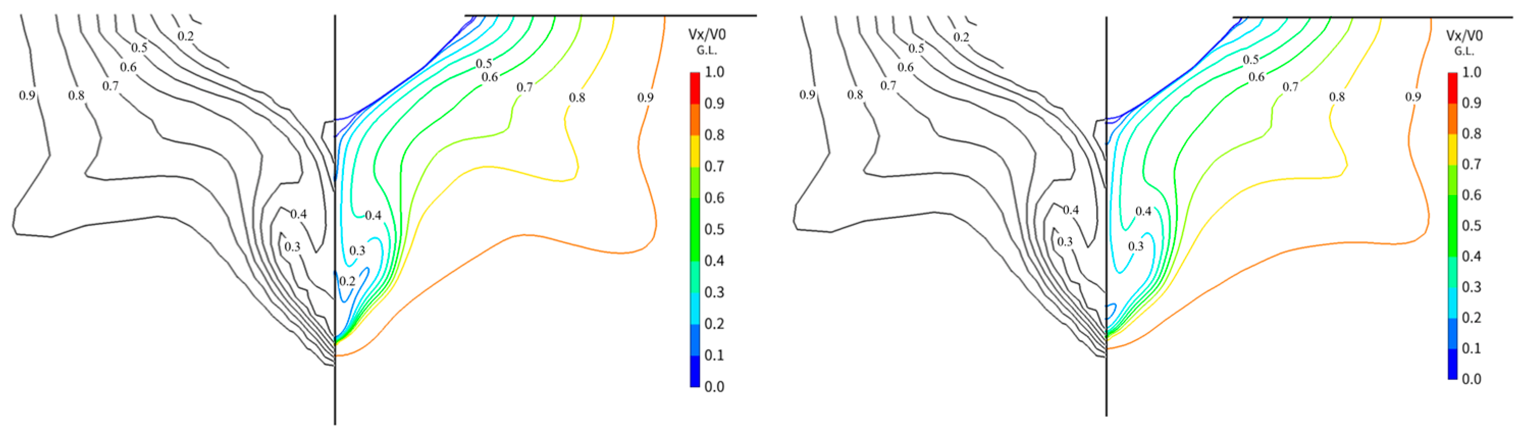
Figure 7. Comparison of contour line of Vx/V0 ((left): k-omega SST; (right): RSM-LPST).

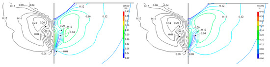
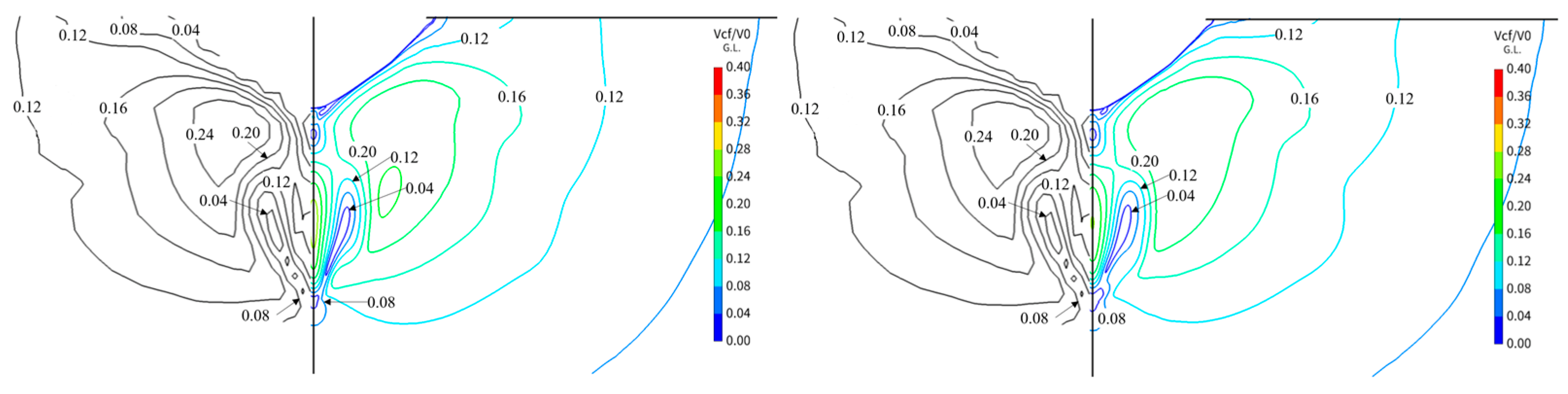
Figure 8. Comparison of contour line of $V_{cf}$/V0 ((left): k-omega SST; (right): RSM-LPST).

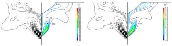
Figure 9. Comparison of contour line of $\overline{u^{\prime }{u}^{\prime }}$ ((left): k-omega SST; (right): RSM-LPST).

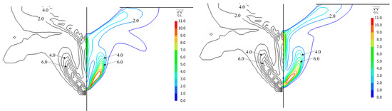
Figure 10. Comparison of contour line of $\overline{v^{\prime }{v}^{\prime }}$ ((left): k-omega SST; (right): RSM-LPST).

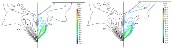
Figure 11. Comparison of contour line of $\overline{w^{\prime }{w}^{\prime }}$ ((left): k-omega SST; (right): RSM-LPST).

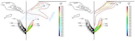
Figure 12. Comparison of contour line of $\overline{u^{\prime }{w}^{\prime }}$ ((left): k-omega SST; (right): LPST).

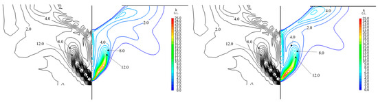
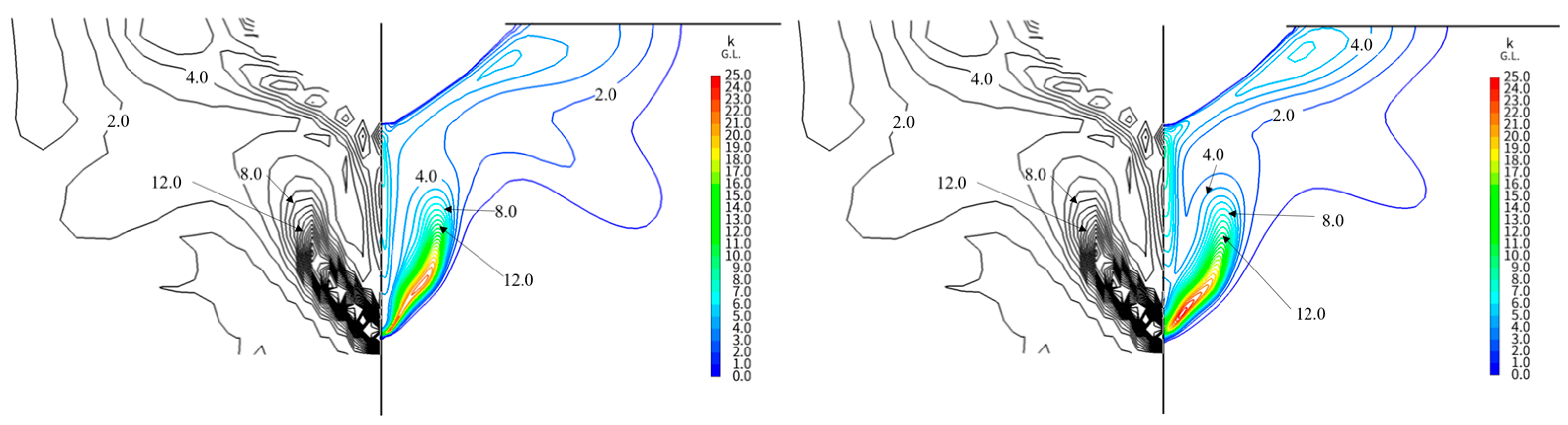
Figure 13. Comparison of contour line of k ((left): k-omega SST; (right): RSM-LPST).

The distribution of crossflow velocity magnitude is a valuable tool for assessing the intensity of longitudinal vortices and identifying their core locations.

As depicted in Figure 7, the Vx/V0 closely aligns between CFD and EFD when contour levels are from 0.5 to 0.9 for both the k-omega SST and RSM-LPST models. Notably, for the k-omega SST, the stern longitudinal vortex area circled by 0.3 and 0.4 lines is smaller than that of the experimental results. Conversely, the RSM-LPST demonstrates a superior correspondence with the 0.3 and 0.4 lines, an observation also noted by Matsuda et al. [3], with a similar trend observed for $V_{cf}$, $\overline{u^{\prime }{u}^{\prime }}$, $\overline{v^{\prime }{v}^{\prime }}$, $\overline{w^{\prime }{w}^{\prime }}$, $\overline{u^{\prime }{v}^{\prime }}$, $\overline{v^{\prime }{w}^{\prime }}$, $\overline{u^{\prime }{w}^{\prime }}$, and k.

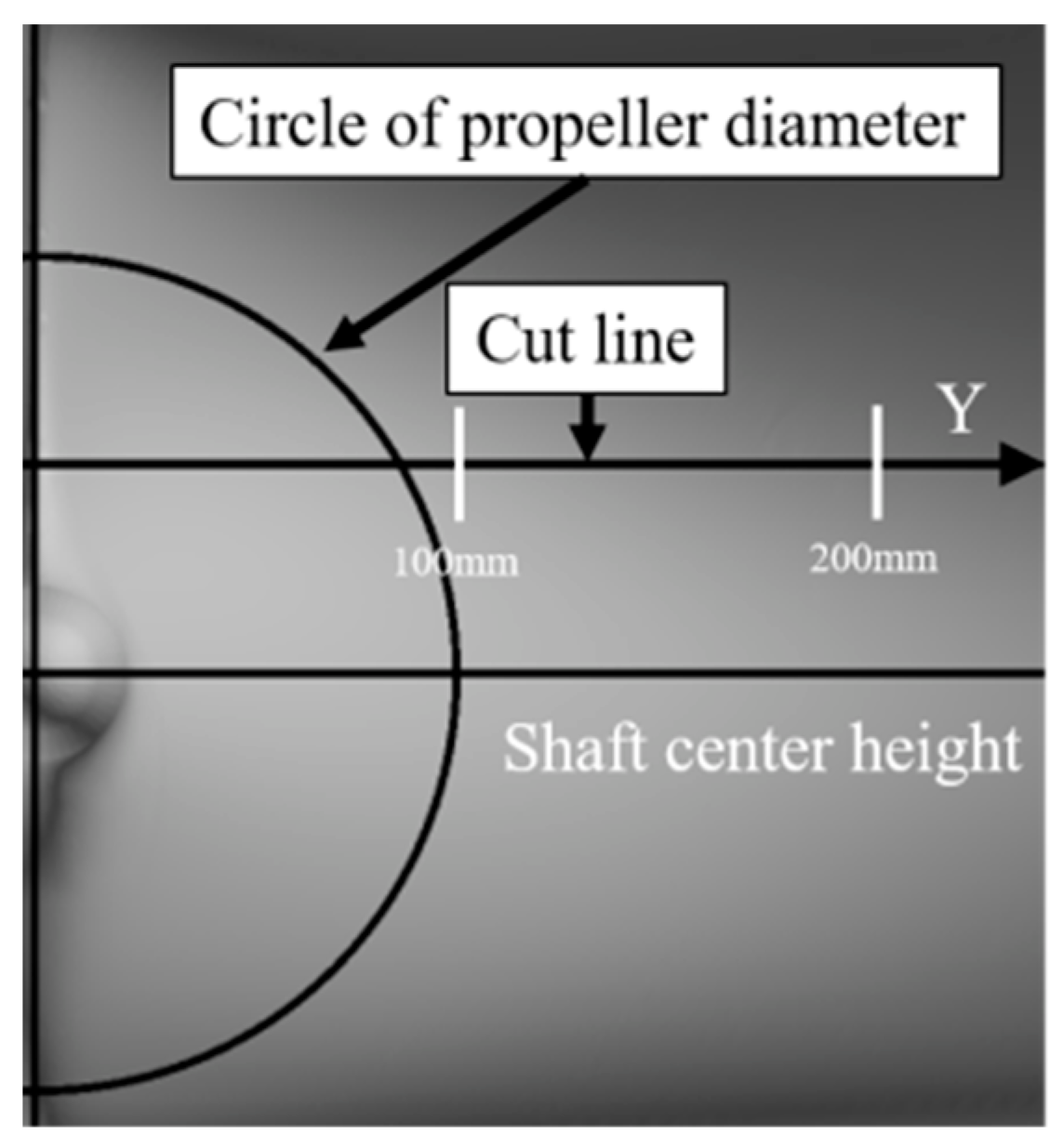
A comparison is presented for a line 0.5R vertically up from the shaft center height for a more detailed comparison between the CFD results of velocity and Reynolds stress distributions and the experimental data. Figure 14 shows the definition and a schematic view of Y (mm). Figure 15, Figure 16, Figure 17 and Figure 18 show the cut line distributions of Vx/V0 and the crossflow velocity, $\overline{u^{\prime }{u}^{\prime }}$, $\overline{v^{\prime }{v}^{\prime }}$, $\overline{w^{\prime }{w}^{\prime }}$, $\overline{u^{\prime }{v}^{\prime }}$, $\overline{v^{\prime }{w}^{\prime }}$, $\overline{u^{\prime }{w}^{\prime }}$, and k.

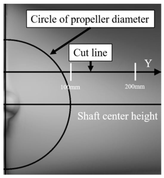
Figure 14. Schematic view of cut line.

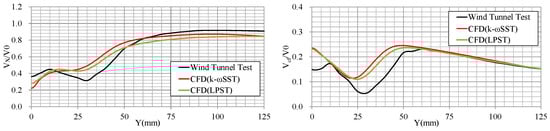
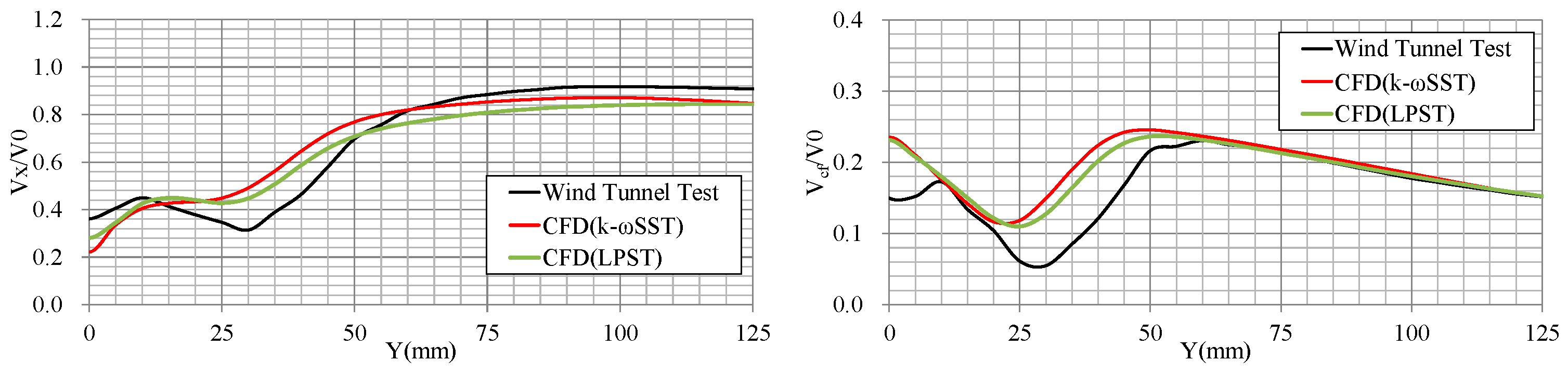
Figure 15. Velocity distribution along horizontal line above propeller shaft ((left): Vx/V0; (right): $V_{cf}$).

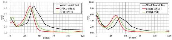
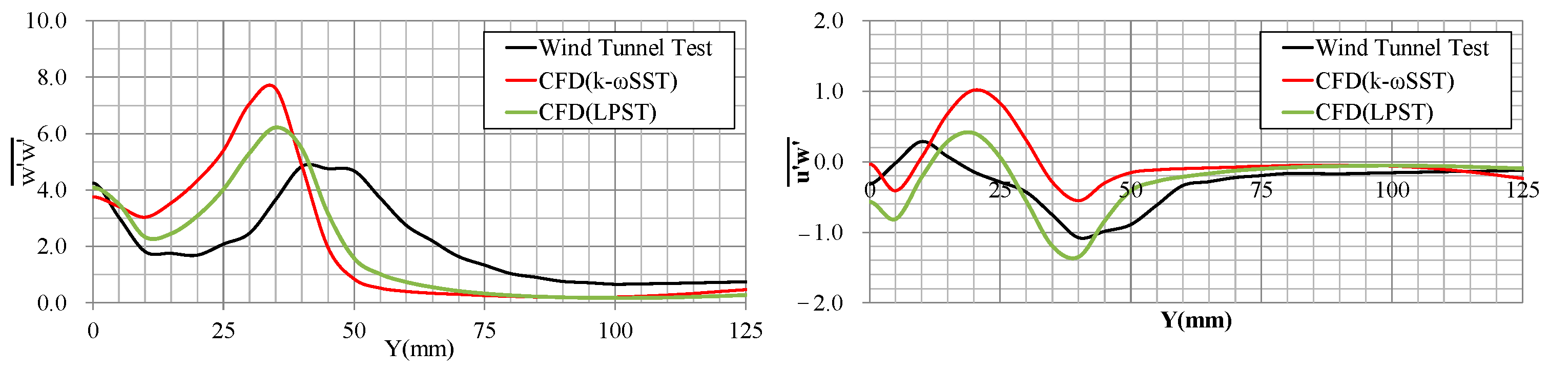
Figure 16. Reynolds stress distribution along horizontal line above propeller shaft ((left): $\overline{u^{\prime }{u}^{\prime }}$; (right): $\overline{v^{\prime }{v}^{\prime }}$).

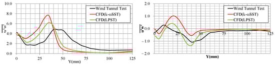
Figure 17. Reynolds stress distribution along horizontal line above propeller shaft ((left): $\overline{w^{\prime }{w}^{\prime }}$; (right): $\overline{u^{\prime }{w}^{\prime }}$).

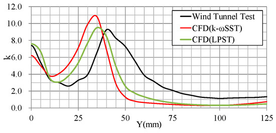
Figure 18. k distribution along horizontal line above propeller shaft.

As shown in Figure 15, Figure 16, Figure 17 and Figure 18, the RSM-LPST is closer to EFD from Y = 0 to 75 mm. The peak magnitude and location of the RSM-LPST closely resembles the EFD values for the k-omega SST in terms of $\overline{u^{\prime }{u}^{\prime }}$, $\overline{v^{\prime }{v}^{\prime }}$, $\overline{w^{\prime }{w}^{\prime }}$, $\overline{u^{\prime }{w}^{\prime }}$, and k. On the other hand, the range above Y = 75 mm is almost the same for both turbulence models.

The results of CFD computations on the 3 m model indicate that the RSM-LPST tends to exhibit closer agreement with the experimental results compared to the k-omega SST. This confirms the efficacy of the RSM-LPST in achieving more accurate predictions.

3. Full-Scale Calculation of Ship Flow Considering Hull Surface Roughness

To assess the accuracy of predicting wake flow distribution at full-scale Reynolds numbers using the RSM, CFD computations were conducted for the same vessel as in the previous section, the Ryuko-maru. The measured data of the full-scale wake flow distribution for the Ryuko-maru are publicly available in Ogiwara [17], enabling a direct comparison with the calculated results. The calculations were performed using the RSM–LPS, incorporating a wall function to account for hull surface roughness. Extensive research on roughness functions, particularly for sand roughness, supports using this method owing to its high estimation accuracy, as highlighted by Ohashi [9]. Consistent with Ohashi’s findings, CFD simulations were performed under towing conditions, given the negligible impact of propeller suction in this scenario. Although only the roughness of the hull is considered here, the propeller in high-roughness conditions will affect the resistance as well as the power required.

3.1. Roughness Function

Surface friction increases in the presence of surface roughness compared to a smooth surface. This effect is evidenced by a reduced mean velocity distribution within the turbulent boundary layer, a phenomenon quantified by the roughness function $\mathsf{\Delta }{U}^{+}$. The dimensionless velocity distribution within the logarithmic law domain of a rough surface is expressed by Equation (2) proposed by Cebeci and Bradshaw [18]:

$$U^{+}=\frac{1}{\kappa }\ln \left(y^{+}\right)+B-\mathsf{\Delta }{U}^{+}$$

(2)

where $\kappa$ is the von Karman constant, $y^{+}$ is the nondimensional normal distance from the boundary, B is the smooth wall log–law intercept, and $\mathsf{\Delta }{U}^{+}$ is the roughness function. The roughness function varies with the roughness characteristics and is determined as a function of the roughness Reynolds number $k^{+}$, as in Equation (3), used in Star-CCM+ [19]. The definition of $k^{+}$ is shown in Equation (4).

$$\mathsf{\Delta }{U}^{+}=\left\{\begin{array}{c}0, k^{+}\le k_{smooth}^{+}\\ \frac{1}{\kappa }\ln {\left[C_1\left(\frac{k^{+}-k_{smooth}^{+}}{k_{Rough}^{+}-k_{smooth}^{+}}\right)+C_2{k}^{+}\right]}^{\alpha },k_{smooth}^{+}<k^{+}<k_{Rough}^{+}\\ \frac{1}{\kappa }\ln \left(C_1+C_2{k}^{+}\right), k^{+}>k_{Rough}^{+}\end{array}\right.$$

(3)

where:

$\alpha =sin\left[\frac{\pi }{2}\frac{\mathrm{l}\mathrm{o}\mathrm{g}(k^{+}/k_{smooth}^{+})}{\mathrm{l}\mathrm{o}\mathrm{g}\left(k_{Rough}^{+}/k_{smooth}^{+}\right)}\right]$.

$$k^{+}=\frac{u_{\tau }{k}_s}{\nu }$$

(4)

where $u_{\tau }$ is the friction velocity, $k_s$ is the characteristic roughness length scale, and $\nu$ is the kinematic viscosity. As shown in Table 6, various coefficients have been proposed with $k_{smooth}^{+}$, $k_{Rough}^{+}$, $C_1$, and $C_2$ as parameters. Yigit Karmel Demirel et al. (2014) [20] and Soonseok Song et al. [21] used the same parameters as the default parameter of Star-ccm+. Yigit et al. (2017) [22] calibrated their coefficients to align with the experimental findings of Schultz et al. [23] Andrea Farkas et al. [24] and Henrik Mikkelsen et al. [25] also used the same parameters. Roberto et al. [26] juxtaposed the parameters of White et al. [27] and Grigson [28], as illustrated in Figure 19. In our investigation, we adopted the values from Yigit et al. (2017) and fine-tuned them to accommodate the lower $k^{+}$ range.

Table 6. Table of the coefficients of roughness function.

	C1	C2	k+smooth	k+rough
STAR-CCM+ [19] Yigit Kemal Demirel (2014) [20] Soonseok Song (2021) [21]	0.000	0.253	2.25	90.00
Yigit Kemal Demirel (2017) [22] Andrea Farkas (2019) [24] Henrik Mikkelsen (2020) [25]	0.000	0.260	3.00	15.00
Roberto Ravenna (2022) [26]	−3.000	0.490	3.00	25.00
White (2006) [27]	1.000	0.300
Grigson (1992) [28]	1.000	1.000

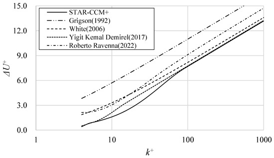
Figure 19. Comparison of roughness function models ([19,22,26,27,28]).

3.2. Condition of Full-Scale CFD

The conditions for conducting full-scale CFD calculations are shown in Table 7, mirroring those employed in the full-scale experiment conducted by Namimatsu et al. [12]. The calculation methodology remained consistent with that outlined in Section 2.

Table 7. A list of the calculation condition of the objective ships.

Lpp (m)	300
B (m)	50
d (m)	18.86
$\nabla$ (m3)	233,554
S (m2)	23,116
ρ (kg/m3)	1027.3
V (m/s)	8.334
ν × 10−5 (m2/s)	0.098608
Rn × 109	2.54

The resulting computations were juxtaposed with the results of the pitot tube measurements of wake flow at the full scale. The turbulence models employed encompassed the k-omega SST and the RSM-LPS.

3.3. Results of CFD Calculation

Initially, smooth conditions and full-scale verifications were conducted. Table 8 presents the grid count and grid refinement ratio $r_i$. Table 8 shows the calculated resistance results. Verification analyses are detailed in Table 9 and Table 10.

Table 8. Results of grid refinement ratio $r_i$ at full scale.

Fine	NC1	38,523,207
Midium	NC2	15,457,974
Coarse	NC3	6,315,456
	Ri	1.352
	Ri,21	1.356
	Ri,32	1.348

Table 9. Results of CFD calculation at full scale.

Turbulance Model	Grid	Fall (N)	Fvis (N)	CT × 103	Cf × 103
k-ω SST	Coarse	1,414,782	1,140,107	1.716	1.383
	Midium	1,413,533	1,140,192	1.714	1.383
	Fine	1,406,526	1,140,616	1.706	1.383
LPS	Coarse	1,501,705	1,194,031	1.821	1.448
	Midium	1,501,398	1,193,697	1.821	1.447
	Fine	1,507,254	1,193,783	1.828	1.448

Table 10. Results of verification of full scale.

	δi	δfine (%(1 + K)fine)	${\mathit{U}}_{\mathit{i}}$	${\mathit{U}}_{\mathit{S}\mathit{N}}$ (%(1 + K)fine)
k-ω SST	0.0103	0.83%	0.0309	1.81%
LPS	-	-	0.0036	0.28%

As indicated in Table 10, the $U_{SN}$ was approximately 1.5% smaller for the RSM-LPS than for the k-omega SST. However, the difference in $U_{SN}$ is negligible for both cases. Consequently, the medium grid was selected for this calculation.

Surface roughness was varied from 29 to 150 μm under smooth surface conditions, and the corresponding current distribution was compared to determine the surface roughness that closely approximated the $\Delta C_F$ predicted by the ITTC 1990 equation (Equation (5)). Additionally, Figure 20 displays graphs depicting $\Delta C_F$ on the horizontal axis and $ks$ (μm) on the vertical axis.

$$\Delta C_F\times {10}^{-3}=44\left[{\left(\frac{ks}{L_{pp}}\right)}^{\frac{1}{3}}-10{Rn}^{-\frac{1}{3}}\right]+0.125$$

(5)

where $ks$ is the roughness of the surface (μm), $L_{pp}$ is the perpendicular length (m), and $Rn$ is the Reynolds number.

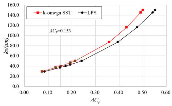
Figure 20. Result of CFD calculation.

As depicted in Figure 20, although both the k-omega SST and the RSM-LPS exhibit a similar trend for $\Delta C_F$, $ks$ is larger for the k-omega SST. Specifically, according to the ITTC 1990 equation, $\Delta C_F$ = 0.153 × 10⁻³ corresponds to $ks$ = 40 μm for the k-omega SST and $ks$ = 37 μm for the RSM-LPS.

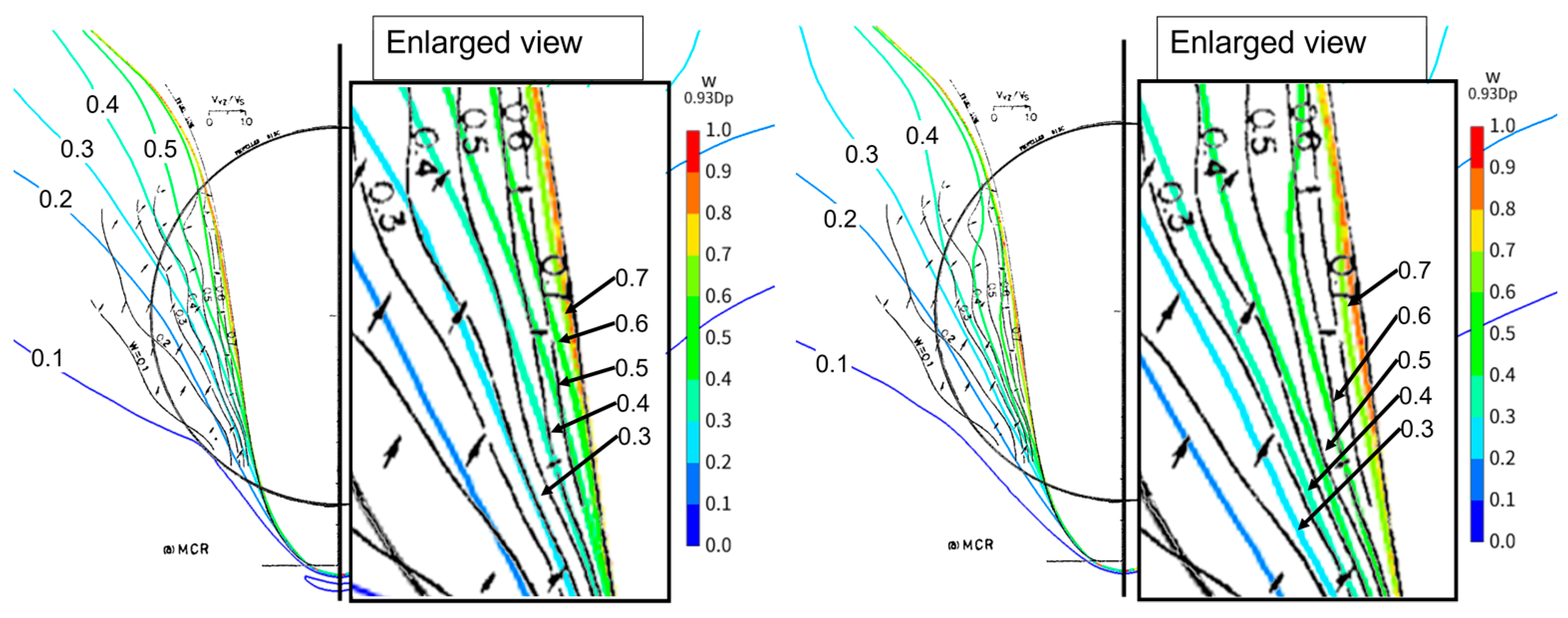
Figure 21, Figure 22 and Figure 23 compare the experimental results and the CFD-estimated wake distribution. Figure 21 displays the calculation results under smooth conditions, while Figure 22 shows the calculation results for $ks$ = 150 (μm). Figure 23 depicts the results for $\Delta C_F$ = 0.153 × 10⁻³. Here, the Vx/V0 contour is juxtaposed with the results of the full-scale measurements (indicated by the black line).

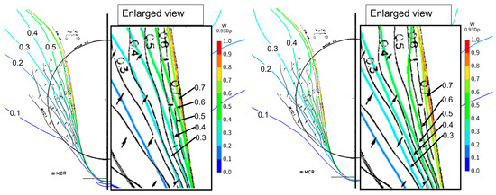
Figure 21. Comparison of results of wake distribution at full scale under smooth conditions ((left): k-omega SST; (right): RSM-LPS).

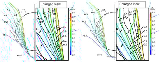
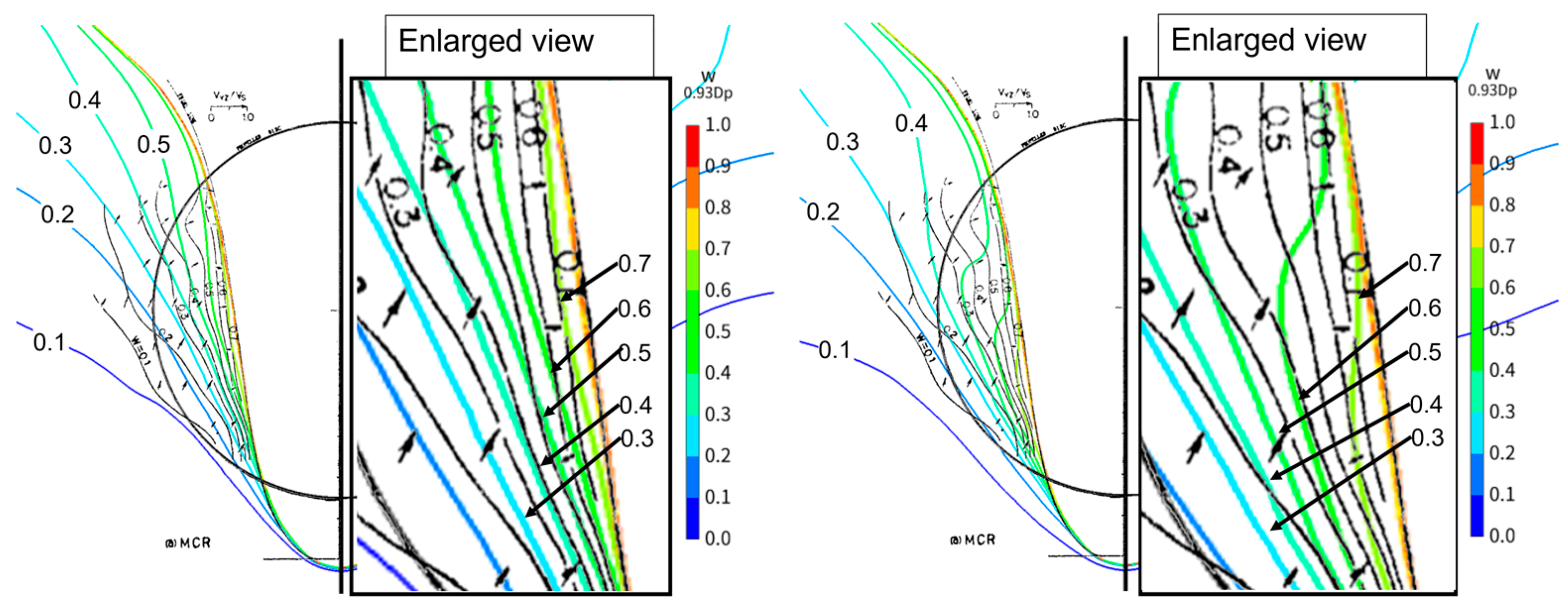
Figure 22. Comparison of results of wake distribution at full scale under rough conditions ((left): k-omega SST ($ks$ = 150 μm); (right): RSM-LPS ($ks$ = 150 μm)).

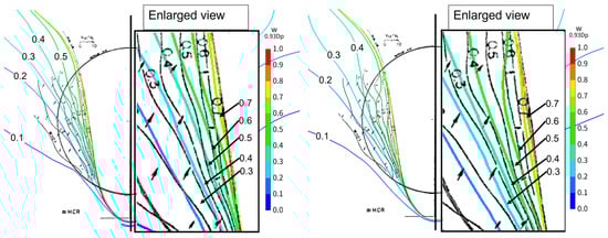
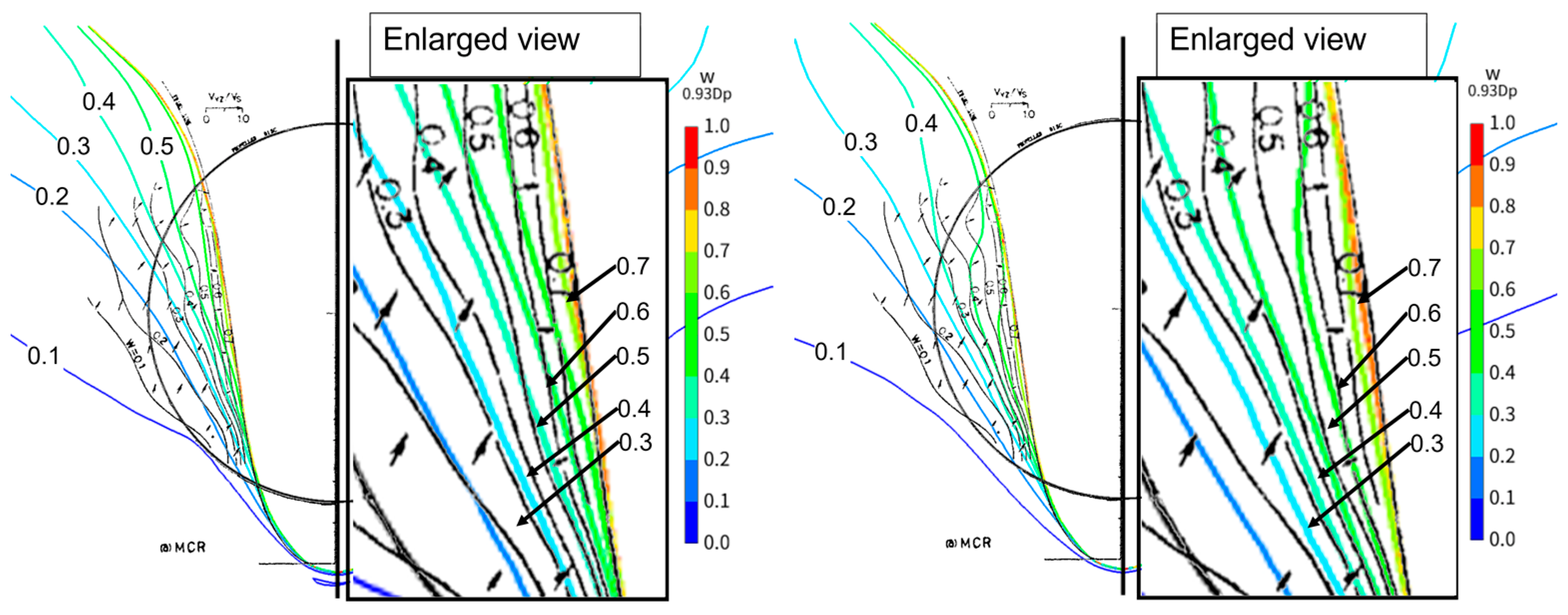
Figure 23. Comparison of results of wake distribution at full scale under rough conditions ((left): k-omega SST ($ks$ = 40 μm); (right): RSM-LPS ($ks$ = 37 μm)).

A notable difference emerges after comparing the calculation results on smooth surfaces, as illustrated in Figure 21. Specifically, the k-omega SST has a thin wake flow at lines above 0.3 compared to the experimental results. The RSM-LPS demonstrates closer agreement between the CFD calculation results and the experimental findings, particularly between the 0.2 and 0.4 lines. Also, the LPS shows a bulge of the boundary layer near the center of the shaft. Above the propeller center, the results from the full-scale ship tests exhibit a wave-shaped pattern, which is not replicated by the trend observed in both CFD calculations. In Figure 22, setting $ks$ to 150 μm resulted in the $\Delta C_F$ of the k-omega SST exceeding twice the ITTC recommendation at the full-scale Reynolds number. However, the wake flow distribution showed good agreement. The LPS estimated the wake flow to be thicker than that of the experimental results. As shown in Figure 23, using $\Delta C_F$ of the ITTC recommendation to account for surface roughness, the LPS results show nearly the same wake distribution (0.4–0.6 lines) near the hull surface. The k-omega SST showed a thinner wake distribution (0.4–0.6 lines) near the hull compared to the experimental results. However, above the propeller center, the k-omega SST showed better agreement. These results show that the RSM-LPS has an advantage over the k-omega SST in terms of separation phenomena and is able to estimate the viscous resistance and the wake distribution of the full-sized vessel with high accuracy.

4. Conclusions

In this study, CFD calculations of the Ryuko-maru employing the RSM were conducted to enhance the accuracy of wake distribution estimation. The CFD calculation results at the model scale were juxtaposed with the Reynolds stress distribution measured in wind tunnel tests. Additionally, the CFD calculation results accounting for full-scale roughness effects were compared with those of full-scale wake flow measurements. These findings are summarized as follows.

• The CFD calculations at the model scale revealed that the RSM–LPST exhibited slightly higher accuracy in predicting the wake flow around the stern longitudinal vortex compared to the k-omega SST.
• Full-scale calculations under smooth conditions demonstrated that the k-omega SST exhibited higher velocities than the measured values with almost no hook shape.
• Setting $ks$ to 150 μm resulted in the $\Delta C_F$ of the k-omega SST exceeding twice the ITTC recommendation at the full-scale Reynolds number. However, the wake flow distribution showed good agreement.
• When $ks$ was adjusted to match the $\Delta C_F$ of the ITTC recommendation, the wake flow near the hull surface displayed good agreement with the RSM-LPS. However, above the propeller center, the k-omega SST showed better agreement.
• The RSM-LPS has an advantage over the k-omega SST in terms of separation phenomena at the full scale and is able to estimate the viscous resistance and the wake distribution of the full-sized vessel with high accuracy.

Based on the findings outlined above and considering computational costs, it is advisable to utilize the RSM–LPS or the LPST to achieve highly accurate predictions close to the hull in full-scale ships. For a more comprehensive validation of the calculation accuracy of the stern longitudinal vortex, it is imperative to acquire measurement results of the full-scale wake distribution close to the propeller.

References

- MEPC. 2023 IMO Strategy on Reduction of GHG Emissions from Ships. MEPC 80/WP.12 Annex 1. 2023. Available online: https://wwwcdn.imo.org/localresources/en/MediaCentre/PressBriefings/Documents/Resolution%20MEPC.377(80).pdf (accessed on 27 March 2024).
- Pena, B.; Huang, L. A review on the turbulence modelling strategy for ship hydrodynamic simulations. Ocean Eng. 2021, 241, 110082. [Google Scholar] [CrossRef]
- Matsuda, S.; Katsui, T. Hydrodynamic Forces and Wake Distribution of Various Ship Shapes Calculated Using a Reynolds Stress Model. J. Mar. Sci. Eng. 2022, 10, 777. [Google Scholar] [CrossRef]
- Korkmaz, K.B.; Werner, S.; Bensow, R. Verification and Validation of CFD Based Form Factors as a Combined CFD/EFD Method. J. Mar. Sci. Eng. 2021, 9, 75. [Google Scholar] [CrossRef]
- Korkmaz, K.B.; Werner, S.; Sakamoto, N.; Queutey, P.; Deng, G.; Gao, Y.; Dong, G.; Maki, K.; Ye, H.; Akinturk, A.; et al. CFD based form factor determination method. Ocean Eng. 2021, 220, 108451. [Google Scholar] [CrossRef]
- Andersson, J.; Shiri, A.A.; Bensow, R.E.; Jin, Y.; Wu, C.; Qiu, G.; Deng, G.; Queutey, P.; Yan, X.-K.; Horn, P.; et al. Ship-scale CFD benchmark study of a pre-swirl duct on KVLCC2. Appl. Ocean Res. 2020, 123, 103134. [Google Scholar] [CrossRef]
- Song, S.; Demirel, Y.K.; Muscat-Fenech, C.D.M.; Tezdogan, T.; Atlar, M. Fouling effect on the resistance of different ship types. Ocean Eng. 2020, 216, 107736. [Google Scholar] [CrossRef]
- Pena, B.; Muk-Pavic, E.; Fitzsimmons, P. Detailed analysis of the flow within the boundary layer and wake of a full-scale ship. Ocean Eng. 2020, 218, 108022. [Google Scholar] [CrossRef]
- Ohashi, K. Numerical study of roughness model effect including low-Reynolds number model and wall function method at actual ship scale. J. Mar. Sci. Technol. 2021, 26, 24–36. [Google Scholar] [CrossRef]
- Sakamoto, N.; Kobayashi, H.; Ohashi, K.; Kawanami, Y.; Windén, B.; Kamiirisa, H. An overset RaNS prediction and validation of full scale stern wake for 1,600TEU container ship and 63,000 DWT bulk carrier with an energy saving device. Appl. Ocean Res. 2020, 105, 102417. [Google Scholar] [CrossRef]
- Suzuki, H.; Miyazaki, S.; Suzuki, T.; Matsumura, K. Turbulence Measurements in Stern Flow of Ship Models–Ryuko-maru (Tanker form), Hamburg Test Case (Container form). J.-Kansai Soc. Nav. Archit. Jpn. 1998, 230, 109–122. (In Japanese) [Google Scholar]
- Namimatsu, M.; Muraoka, K.; Yamashita, S.; Kushimoto, H. Wake Distribution of Ship and Model on Full Ship Form. J. Soc. Nav. Archit. Jpn. 1973, 134, 65–73. (In Japanese) [Google Scholar] [CrossRef]
- Gibson, M.M.; Launder, B.E. Ground effects on pressure fluctuations in the atmospheric boundary layer. J. Fluid Mech. 1978, 86, 491–511. [Google Scholar] [CrossRef]
- Launder, B.E.; Shima, N. Second Moment Closure for the Near-Wall Sublayer. Dev. Appl. AIAA J 1989, 27, 1319–1325. [Google Scholar] [CrossRef]
- Rodi, W. Experience with Two-Layer Models Combining the k-e Model with a One-Equation Model Near the Wall. In Proceedings of the 29th Aerospace Sciences Meeting, Reno, NV, USA, 7–10 January 1991. AIAA 91-0216. [Google Scholar]
- ITTC. Recommended procedures and guidelines—Uncertainty analysis in CFD verification and validation methodology and procedures. In Proceedings of the 28th International Towing Tank Conference, Wuxi, China, 17–22 September 2017. [Google Scholar]
- Ogiwara, S. Stern Flow Measurements for the Tanker ‘Ryuko-Maru’ in Model Scale, Intermediate Scale, and Full Scale Ships. Proc. CFD Workshop Tokyo 1994, 1, 341–349. [Google Scholar]
- Cebeci, T.; Bradshaw, P. Momentum Transfer in Boundary Layers; Hemisphere Publishing Corp.: Washington, DC,, USA; McGraw-Hill Book Co.: New York, NY, USA, 1977. [Google Scholar]
- Siemens Digital Industries Software. User Guide Simcenter STAR-CCM+ 2021.1. Available online: https://docs.sw.siemens.com/ja-JP/doc/226870983/PL20201109101148301.starccmp_installguide_pdf?audience=external&pk_vid=2d7d3ecf2bbd1d6f4858ceeeb21cee311714744815a1775a (accessed on 27 March 2024).
- Demirel, Y.K.; Khorasanchi, M.; Turan, O.; Incecik, A.; Schultz, M.P. A CFD model for the frictional resistance prediction of antifouling coatings. Ocean Eng. 2014, 89, 21–31. [Google Scholar] [CrossRef]
- Song, S.; Ravenna, R.; Dai, S.; Muscat-Fenech, C.D.; Tani, G.; Demirel, Y.K.; Atlar, M.; Day, S.; Incecik, A. Experimental investigation on the effect of heterogeneous hull roughness on ship resistance. Ocean Eng. 2021, 223, 108590. [Google Scholar] [CrossRef]
- Demirel, Y.K.; Turan, O.; Incecik, A. Predicting the effect of biofouling on ship resistance using CFD. Appl. Ocean Res. 2017, 62, 100–118. [Google Scholar] [CrossRef]
- Schultz, M.P.; Flack, K.A. The Rough-Wall Turbulent Boundary Layer from the Hydraulically Smooth to the Fully Rough Regime. J. Fluid Mech. 2007, 580, 381–405. [Google Scholar] [CrossRef]
- Farkas, A.; Degiuli, N.; Martić, I.; Dejhalla, R. Numerical and experimental assessment of nominal wake for a bulk carrier. J. Mar. Sci. Technol. 2019, 24, 1092–1104. [Google Scholar]
- Mikkelsen, H.; Walther, J.H. Effect of roughness in full-scale validation of a CFD model of self-propelled ships. Appl. Ocean Res. 2020, 99, 102162. [Google Scholar] [CrossRef]
- Ravenna, R.; Song, S.; Shi, W.; Sant, T.; Muscat-Fenech, C.D.M.; Tezdogan, T.; Demirel, Y.K. CFD analysis of the effect of heterogeneous hull roughness on ship resistance. Ocean Eng. 2022, 258, 111733. [Google Scholar] [CrossRef]
- White, F.M.; Majdalani, J. Viscous Fluid Flow; McGraw-Hill: New York, NY, USA, 2006; Volume 3. [Google Scholar]
- Grigson, C. Drag losses of new ships caused by hull finish. J. Ship Res. 1992, 36, 182–196. [Google Scholar] [CrossRef]
Disclaimer/Publisher’s Note: The statements, opinions and data contained in all publications are solely those of the individual author(s) and contributor(s) and not of MDPI and/or the editor(s). MDPI and/or the editor(s) disclaim responsibility for any injury to people or property resulting from any ideas, methods, instructions or products referred to in the content. |
© 2024 by the authors. Licensee MDPI, Basel, Switzerland. This article is an open access article distributed under the terms and conditions of the Creative Commons Attribution (CC BY) license (https://creativecommons.org/licenses/by/4.0/).