Prescribed Performance Formation Tracking Control for Underactuated AUVs under Time-Varying Communication Delays

Abstract

Achieving formation tracking control of underactuated autonomous underwater vehicles (AUVs) under communication delays presents a significant challenge. To address this challenge, a distributed prescribed performance control protocol based on a real-time state information online predictor (RSIOP) is proposed in this paper. First, we innovatively designed an RSIOP to achieve active compensation for the delayed state information of neighboring AUVs. Next, considering formation performance and safety, a low-complexity and practical nonlinear mapping function was used to implement prescribed performance tracking control for the AUV formation. Additionally, the adverse effects of external disturbance uncertainties and input saturation are also considered. Finally, the simulation tests demonstrated that the proposed formation control protocol can successfully achieve the predetermined formation tracking tasks in the presence of time-varying communication delays and external disturbances, while also enabling real-time changes in formation configuration during the process. Throughout, the protocol maintains input saturation limits, and the actual control inputs remain smooth, with no significant oscillations. Furthermore, comparative simulation tests verified the necessity of the RSIOP developed in this study and quantitatively demonstrated that the proposed control method exhibits superior performance in terms of formation control accuracy, error convergence speed, and transient-state constraints.

1. Introduction

Autonomous underwater vehicles (AUVs) constitute an emerging class of unmanned underwater platforms that have experienced rapid advancements in recent years, driven by significant progress in energy systems, sensing technologies, navigation, communication, and control technologies [1,2,3,4,5]. However, with the expansion of oceanic endeavors and the increasing complexity of underwater tasks, AUVs face significant challenges. The limited energy capacity, the susceptibility to ocean currents and marine life disturbances, and the relatively small operational coverage within a limited timeframe of single AUV platforms are inadequate to meet the requirements of more complex, real-time, large-scale marine missions [6,7]. These limitations highlight the urgent need for more robust and scalable solutions, driving the focus toward multi-AUV systems. Today, multi-AUV systems have been proven to collect more reliable data and exhibit higher efficiency, better fault tolerance, greater robustness, wider mission execution areas, and lower system costs compared to single AUVs [8,9,10,11]. Despite these advantages, the successful deployment of multi-AUV systems poses considerable challenges, especially with respect to formation control and communication reliability. The primary objective of AUV formation control is to manage the relative distance, speed, or orientation between AUVs, enabling them to move as a unified group. This facilitates tasks such as transitioning from initial positions to a designated location to form a specific formation or maintaining a certain formation during navigation [12].

The success of AUV formation control relies heavily on effective communication between vehicles. To achieve AUV formation, information transmission between AUVs must be conducted through wireless communication within a network control system. Acoustic communication has become the most widely used method due to its advantages of longer underwater propagation distances and lower attenuation. However, due to its relatively slow transmission speed and the time required for data parsing, underwater communication is subject to significant delays. This results in each AUV receiving the delayed state of neighboring AUVs rather than accurate, real-time states. These delays can severely impact the control performance and stability of the formation control system, making it a crucial challenge that must be addressed [13,14]. Recent research has made progress in addressing the challenges posed by communication delays, yet significant gaps remain. Li et al. [15,16] established the Lyapunov–Krasovskii equation and used linear matrix inequality (LMI) to solve the time-varying communication delay problem, obtaining boundary conditions for control system error convergence. Zhang et al. [17] modeled a fixed communication topology and, combined with a consensus algorithm, proposed a leader–follower control strategy designed to handle time-varying delays, establishing new stability criteria to ensure the consistency of multi-AUV systems. Zeng et al. [18], utilizing matrix theory and pertinent stability criteria, established sufficient conditions for the stability of the error system under both scenarios, with and without communication delays. Yan et al. [19] proposed a multi-UUV path-following controller based on a virtual leader to address communication delays, using Shuler theory to provide sufficient conditions for multi-UUV path-following convergence. While these approaches have advanced the field, they primarily rely on the delayed states of neighboring AUVs and require knowledge of the upper bound of communication delays. As a result, they address the communication delay problem between AUVs in a passive manner, which limits their effectiveness in more dynamic environments and presents certain limitations. Li et al. [20] studied fully actuated AUVs and used curve-fitting methods to predict the leader’s state in a two-dimensional formation, but the fixed-order model used had difficulties ensuring prediction accuracy. Du et al. [21] pioneered an active communication delay compensation mechanism by designing a data-driven state predictor to estimate the current motion state of neighboring AUVs in real-time. However, the recursive step size of state estimation is dependent on the order of the prediction model, which can result in prediction failures due to data loss, making it potentially less suitable for practical AUV applications.

Moreover, another critical aspect of AUV formation control is the management of formation state errors, which has direct implications for system performance and safety. While several approaches have been proposed, challenges remain. Bechlioulis et al. [22] initially introduced an innovative approach known as prescribed performance control (PPC) for nonlinear systems. By transforming the constrained nonlinear system under the prescribed performance function into an unconstrained one, they designed a robust controller to maintain the error within predefined performance bounds. This method set a foundation, yet it involves intricate transformations and handling of constraints. Since then, numerous scholars have conducted research building upon this approach. For instance, Liu et al. [23] transformed tracking errors into virtual errors using a specified performance function and designed an adaptive region-tracking control scheme with transient performance using backstepping technology. Similarly, Sun et al. [24] created a PPC strategy for trajectory tracking control of fully actuated AUVs, utilizing performance functions and corresponding error transformations. While effective, these methods share a common drawback: the need for complex transformations to manage constrained tracking errors, which can complicate implementation and limit practical applicability. Recognizing these challenges, Huang et al. [25] used nonlinear mapping techniques to reduce the complexity of designing prescribed performance controllers, effectively addressing the PPC problem for underactuated single AUVs. However, even with these improvements, PPCs often require large control inputs at the initial stage. Due to the physical constraints of AUV equipment, actuator input saturation becomes unavoidable, leading to performance degradation [26]. This issue has been overlooked in the aforementioned studies, yet it is clearly a problem that urgently needs to be addressed in formation control. Thus, while significant progress has been made, these limitations underscore the need for further research to develop more practical and robust PPC solutions that can be effectively implemented in real-world AUV formations.

In response to these challenges and research gaps, this paper centers on the formation control of underactuated AUVs and develops a prescribed performance control protocol for formation tracking under time-varying communication conditions. Unlike previous studies, the proposed control protocol offers the following advantages:

(1)

Combining time series analysis theory, an innovative real-time state information online predictor (RSIOP) is proposed. This approach does not necessitate prior knowledge of the upper bound of communication delays. Instead, it leverages the delayed motion state information of neighboring AUVs to recursively obtain their current state information. This approach not only ensures data validity but also achieves real-time active compensation for time-varying communication delays.

(2)

To enhance both transient and steady-state performance, the AUV formation’s motion states are constrained using prescribed performance functions, which significantly improves operational efficiency. Additionally, by incorporating nonlinear mapping techniques, the complex transformations of constrained errors are avoided, resulting in a more straightforward and intuitive control protocol design.

(3)

The proposed approach addresses the adverse effects of input saturation and unknown external disturbances in AUV formation control without the need for observers, thereby simplifying the adjustment of control parameters.

(4)

The formation is designed to be dynamic, enhancing its flexibility in practical applications and improving its ability to adapt to complex and evolving environments.

The rest of this paper is structured as follows. The preliminary and problem formulations are presented in Section 2. Section 3 describes the solution to time-varying communication delays. Section 4 presents the design of the prescribed performance formation tracking controller, along with a stability analysis of the closed-loop system. Section 5 offers the simulation results to validate the effectiveness of the control protocol. Finally, the conclusions are summarized in Section 6.

2. Preliminary and Problem Formulations

2.1. Graphy Theory

Communication topology is a critical component in the formation control of AUVs. It serves as a bridge connecting AUVs, establishing the mechanisms for information flow exchange. Graph theory can be effectively utilized to describe communication topology, providing robust theoretical support for formation control.

In this article, a weighted directed graph $G=\left\{V,E,A\right\}$ is utilized to represent the communication topology among AUVs within the network system. Assume there is a virtual leader and N AUVs in the formation, with each AUV considered as a node. $V=\left\{v_0,v_1,\dots ,v_N\right\}$ represents the set of nodes in the formation, $E\subseteq V\times V$ denotes the set of edges, and $A=\left[a_{ij}\right]\in {ℝ}^{(N+1)\times (N+1)}$ is the weighted adjacency matrix. If an edge $\left(v_i,v_j\right)\in E$, it indicates that information from the $jth$ AUV can flow to the $ith$ AUV, and $a_{ij}$ = 1. The $jth$ AUV can then be referred to as a neighbor of the $ith$ AUV, and the neighbor set of $ith$ vehicle can be denoted as $B_i=\left\{\left.j\right|\left(v_i,v_j\right)\in E\right\}$. $b_i={\displaystyle \sum _{j=0}^N{a}_{ij}}$ specifies the number of neighbors of the $ith$ vehicle. The $a_{ij}$ can be represented as follows:

$$a_{ij}=\left\{\begin{array}{l}1, if\left\{\left(v_i,v_j\right)\in E,i\ne j\right\}\\ 0, otherwise\end{array}\right.$$

Assumption 1.

Within the communication network system, at least one path exists between any two nodes, indicating that G is connected. Additionally, the virtual leader acts as the root node of the system.

2.2. AUV Model

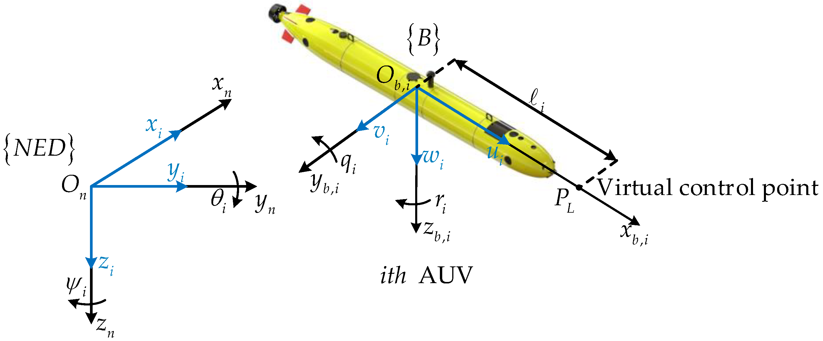
Consider a 5-DOF underactuated AUV mathematical model subject to external disturbances and saturation constraints. The north–east–down frame $\left\{NED\right\}$ and the body-fixed frame $\left\{B\right\}$ of the $ith$ AUV are established separately, as illustrated in Figure 1.

Figure 1. Coordinate frame system of the AUV.

According to reference [27], the three-dimensional motion model of the $ith$ AUV can be derived.

$${\dot{\eta }}_i=J({\eta }_i)v_i$$

(1)

$$M_i{\dot{v}}_i+C_i(v_i)v_i+D_i(v_i)v_i+g_i({\theta }_i)=T_i+{\Delta }_i$$

(2)

where ${\eta }_i={\left[x_i,y_i,z_i,{\theta }_i,{\psi }_i\right]}^T$ denotes the positions (i.e., surge, sway, and heave displacements) and orientations (i.e., pitch and yaw angles) in the north–east–down frame. $v_i={\left[v{u}_i,v_i,w_i,p_i,r_i\right]}^T$ represents the velocities in the body-fixed frame. $J({\eta }_i)$ is the transformation matrix and can be described as

$$J({\eta }_i)=\left[\begin{array}{ccccc}\cos \left({\theta }_i\right)\cos \left({\psi }_i\right) & -\sin \left({\psi }_i\right) & \sin \left({\theta }_i\right)\cos \left({\psi }_i\right)& 0& 0\\ \cos \left({\theta }_i\right)\sin \left({\psi }_i\right)& \cos \left({\psi }_i\right)& \sin \left({\psi }_i\right)\sin \left({\theta }_i\right)& 0& 0\\ -\sin \left({\theta }_i\right)& 0& \cos \left({\theta }_i\right)& 0& 0\\ 0& 0& 0& 1& 0\\ 0& 0& 0& 0& {\displaystyle \frac{1}{\cos ({\theta }_i)}}\end{array}\right]$$

$M_i=diag\left[m_{11,i},m_{22,i},m_{33,i},m_{55,i},m_{66,i}\right]$ is the inertial matrix of the AUV.

$C_i\left(v_i\right)=\left[\begin{array}{ccccc}0& 0& 0& m_{33,i}{w}_i& -m_{22,i}{v}_i\\ 0& 0& 0& 0& m_{11,i}{u}_i\\ 0& 0& 0& -m_{11,i}{u}_i& 0\\ -m_{33,i}{w}_i& m_{11,i}{u}_i& 0& 0& 0\\ m_{22,i}{v}_i& -m_{11,i}{u}_i& 0& 0& 0\end{array}\right]$ is the Coriolis and centripetal matrix.

$D\left(v_i\right)=diag\{X_{u,i},Y_{v,i},Z_{w,i},M_{q,i},N_{r,i}\}$ represents the damping matrix.

$g_i\left({\theta }_i\right)={\left[0,0,0,{\rho }_i{g}_i{\nabla }_{i}G{M}_{L,i}\sin \left({\theta }_i\right),0\right]}^T$ is the restoring moment matrix.

$T_i={\left[T_{1,i},0,0,T_{4,i},T_{5,i}\right]}^T$ denotes the actual input control force.

And ${\Delta }_i={\left[{\Delta }_{1,i},{\Delta }_{2,i},{\Delta }_{3,i},{\Delta }_{4,i},{\Delta }_{5,i}\right]}^T$ is the uncertain external disturbance.

Assumption 2.

For the uncertain external disturbance ${\Delta }_i$, there exists a positive constant ${\overline{\Delta }}_i$ such that $‖{\Delta }_i‖\le {\overline{\Delta }}_i$ always holds.

However, to address the underactuation problem, a coordinate transformation is required to integrate the dynamics in all directions and involve all control inputs [28].

$$y_i=H_i\left({\eta }_i\right)={\left[x_i+{\mathit{\ell }}_i\cos \left({\theta }_i\right)\cos \left({\psi }_i\right),y_i+{\mathit{\ell }}_i\cos \left({\theta }_i\right)\sin \left({\psi }_i\right),z_i-{\mathit{\ell }}_i\sin \left({\theta }_i\right)\right]}^T$$

(3)

where ${\mathit{\ell }}_i$ is a constant positive parameter that represents the distance between the virtual control point $P_i$ and the center of mass (COM) along the $O_{b,i}{x}_{b,i}$ axis, as illustrated in Figure 1. Furthermore, by differentiating Equation (3) and incorporating Equations (1) and (2), the new kinematic and dynamic equations for the AUV can be obtained.

$${\dot{\eta }}_i^{*}=J_{1,i}^{*}\left({\eta }_i\right)v_i^{*}+J_{2,i}^{*}\left({\eta }_i,v_i\right)$$

(4)

$${\dot{v}}_i^{*}={\left(M_i^{*}\right)}^{-1}\left(T_i^{*}+{\Delta }_i^{*}-C_i^{*}\left(v_i\right)v_i^{*}-D_i^{*}\left(v_i\right)v_i^{*}-g_i^{*}\left({\theta }_i\right)\right)$$

(5)

where

$$J_{1,i}^{*}\left({\eta }_i\right)=\left[\begin{array}{ccc}\cos \left({\theta }_i\right)\cos \left({\psi }_i\right)& -{\mathit{\ell }}_i\sin \left({\theta }_i\right)\cos \left({\psi }_i\right)& -{\mathit{\ell }}_i\sin \left({\psi }_i\right)\\ \cos \left({\theta }_i\right)\sin \left({\psi }_i\right)& -{\mathit{\ell }}_i\sin \left({\theta }_i\right)\sin \left({\psi }_i\right)& {\mathit{\ell }}_i\cos \left({\psi }_i\right)\\ -\sin \left({\theta }_i\right)& -{\mathit{\ell }}_i\cos \left({\theta }_i\right)& 0\end{array}\right]$$

$$J_{2,i}^{*}\left({\eta }_i,v_i\right)=\left[\begin{array}{c}-v_i\sin \left({\psi }_i\right)+w_i\sin \left({\theta }_i\right)\cos \left({\psi }_i\right)\\ v_i\cos \left({\psi }_i\right)+w_i\sin \left({\theta }_i\right)\sin \left({\psi }_i\right)\\ w_i\cos \left({\psi }_i\right)\end{array}\right]$$

$$C_i^{*}\left(v_i\right)=\left[\begin{array}{ccc}0& m_{33,i}{w}_i& -m_{22,i}{v}_i\\ \left(m_{11,i}-m_{33,i}\right)w_i& 0& 0\\ \left(m_{22,i}-m_{11,i}\right)v_i& 0& 0\end{array}\right]$$

$v_i^{*}={\left[v{u}_i,q_i,r_i\right]}^T, M_i^{*}=diag\left(m_{11,i},m_{44,i},m_{55,i}\right), D_i^{*}=-diag\left(X_{u,i},M_{q,i},N_{r,i}\right), g_i^{*}\left({\theta }_i^{*}\right)=\left[0,{\rho }_i\right.$$g_i{\nabla }_{i}G{M}_{L,i}{\left.\sin \left({\theta }_i\right),0\right]}^T$, $T_i^{*}={\left[T_{1,i},T_{4,i},T_{5,i}\right]}^T$, ${\Delta }_i^{\ast }={\left[{\Delta }_{1,i},{\Delta }_{4,i},{\Delta }_{5,i}\right]}^T.$

2.3. Actuator Dynamics

In practical applications, due to actuator limitations, the actual output force cannot achieve the control command input force. The specific actuator model is shown in Equation (6).

$$T_{x,i}=sat\left(u_{x,i}\right)=\left\{\begin{array}{l}{u}_{x,i}, if u_{x,i\min }\le u_i\le u_{x,i\max }\\ u_{x,i\min }, if u_i<u_{x,i\min }\\ u_{x,i\max }, if u_i>u_{x,i\max }\end{array}\right.$$

(6)

where $u_{x,i}$ is the command control input; $u_i={\left[u_{1,i},u_{5,i},u_{6,i}\right]}^T$ is the command control input vector; and $u_{x,i\min }$ and $u_{x,i\max }$ denote the saturation constraints.

The existence of such hard saturation limits introduces nonlinearity in the input, adding complexity to the subsequent controller design. Building on the ideas from reference [29], a dead-zone operator-based model (DOBM) is employed to reconfigure the saturation phenomenon, which ensures the continuity of the closed-loop control system.

$$h\left(u_{x,i}\right)={\alpha }_{x,i}{u}_{x,i}-{\displaystyle {\int }_0^{{{\rm E}}_{x,i}}{l}_{x,i}\left({\epsilon }_{x,i}\right)d{z}_{\epsilon ,x,i}\left(u_{x,i}\right)}d{\epsilon }_{x,i}$$

(7)

where $l_{x,i}\left({\epsilon }_i\right)$ is a density function that vanishes at a finite horizon $E_{x,i}$ and satisfies $l_{x,i}\left({\epsilon }_i\right)\ge 0 \forall {\epsilon }_i>0$; ${\alpha }_{x,i}$ is a constant parameter, calculated from ${\alpha }_{x,i}={\displaystyle {\int }_0^{E_{x,i}}{l}_{x,i}\left({\epsilon }_{x,i}\right)d}{\epsilon }_{x,i}$; and $d{z}_{\epsilon ,x,i}\left(u_{x,i}\right)$ denotes a dead-zone operator, which is defined as (8). To simplify notation, we denote ${\overline{\omega }}_{x,i}={\displaystyle {\int }_0^{E_{x,i}}{l}_{x,i}\left({\epsilon }_{x,i}\right)d{z}_{\epsilon ,x,i}\left(u_{x,i}\right)}d{\epsilon }_{x,i}$.

$$d{z}_{\epsilon ,x,i}\left(u_{x,i}\right)=\max \left(u_{x,i}-{\epsilon }_{x,i}\right.,\left.\min \left(0,u_{x,i}+{\epsilon }_{x,i}\right)\right)$$

(8)

The dynamic model of the actuator can be formulated by integrating Equations (6)–(8) as follows:

$$T_i^{\ast }={\alpha }_i{u}_i-{\Omega }_i+o_i$$

(9)

where ${\alpha }_i=diag\left[{\alpha }_{1,i},{\alpha }_{4,i},{\alpha }_{5,i}\right]$, ${\Omega }_i={[{\overline{\omega }}_{1,i},{\overline{\omega }}_{4,i},{\overline{\omega }}_{5,i}]}^T$ and $o_i=sat\left(u_i\right)-h\left(u_i\right)$. Subsequently, the relevant lemma, Lemma 1, is presented. Specifically, Lemma 1 elucidates that $l_{x,i}\left({\epsilon }_{x,i}\right)$ and $E_{x,i}$ can be appropriately chosen to approximate the limits of the saturation constraint, provided that $u_{x,i\min }$ and $u_{x,i\max }$ are known. Given that the dead-zone-based model $h\left(u_i\right)$ is continuous, it further implies that $h\left(u_i\right)$ and $o_i$ are bounded.

Lemma 1

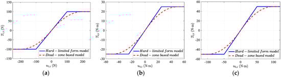
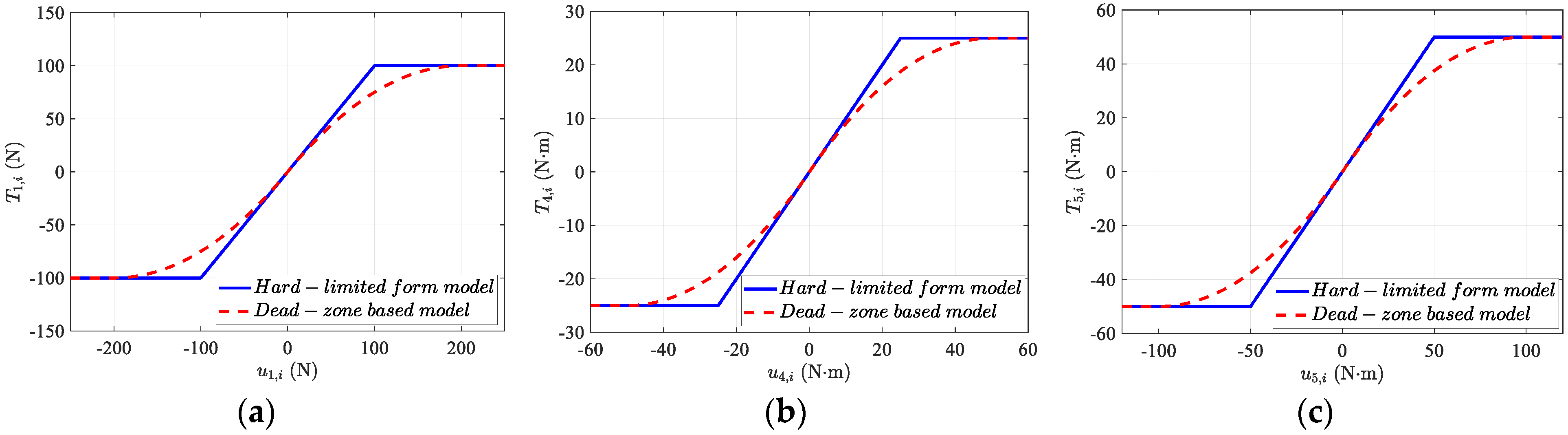
([30]). For any given input saturation limit $u_{x,i,\max }$, there always exists an appropriate density function $l_{x,i}\left({\epsilon }_{x,i}\right)$ ensuring $u_{x,i,\max }=\underset{u_{x,i}\to \infty }{\lim }h\left(u_{x,i}\right)={\displaystyle {\int }_0^{E_{x,i}}{\epsilon }_{x,i}{l}_{x,i}\left({\epsilon }_{x,i}\right)d}{\epsilon }_{x,i}$. The detailed approximation of saturation function effects are illustrated in Figure 2.

Figure 2. Saturation model; here, the density function of the Dead-zone based model is set to $l_{x,i}\left({\epsilon }_{x,i}\right)=\max \left({\mu }_{x,i}sign\left(E_{x,i}-{\epsilon }_{x,i}\right),0\right)$. (a) Consider the scenario where $u_{1,i\max }=-u_{1,i\min }=100$ N with ${\mu }_{1,i}=0.005, E_{1,i}=200$; (b) Consider the scenario where $u_{4,i\max }=-u_{4,i\min }=50$ N·m with ${\mu }_{4,i}=0.01$, $E_{4,i}=100$. (c) Consider the scenario where $u_{5,i\max }=-u_{5,i\min }=25$ N·m with ${\mu }_{5,i}=0.02$, $E_{5,i}=50$.

3. Approach to Address Time-Varying Underwater Acoustic Communication Delay

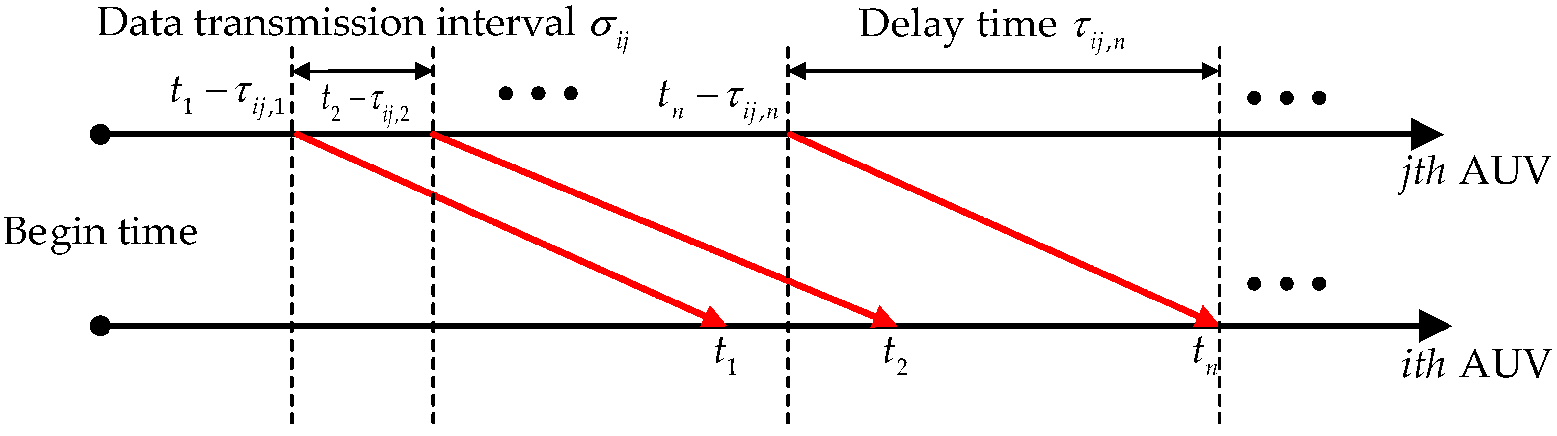
Due to the underwater acoustic communication delay ${\tau }_{ij}$, when the leader $jth$ AUV transmits its state information ${\Phi }_j\left(t\right)$ to the $ith$ AUV, the latter can only receive the delayed state information ${\Phi }_j\left(t-{\tau }_{ij}\right)$ at time $t$, as illustrated in the Figure 3, where the red arrows indicate data information flow transmission.

Figure 3. Data information flow transmission.

Where ${\Phi }_j\left(t\right)=\left[{\eta }_j\left(t\right);v_j\left(t\right)\right]={\left[{\varphi }_{1,j}\left(t\right),{\varphi }_{2,j}\left(t\right),\cdots {\varphi }_{10,j}\left(t\right)\right]}^T$ denotes the state information of j at the moment of data information transmission.

To address the formation-control accuracy issue caused by this delay, an autoregressive model in the form of Equation (10) is introduced to model the AUV state information, inspired by time series theory [31]. The current state information of the jth AUV can be inferred through time series analysis and multi-step prediction.

$${\varphi }_{\rho ,j}\left(t-{\tau }_{ij}\right)={\Phi }_{\rho ,j}^T{\beta }_{\rho ,ij}+{\delta }_{\rho ,ij}$$

(10)

where ${\Phi }_{\rho ,j}={\left[{\varphi }_{\rho ,j}\left(t-{\tau }_{ij}\left(1+1/n_{ij}\right)\right),{\varphi }_{\rho ,j}\left(t-{\tau }_{ij}\left(1+2/n_{ij}\right)\right),\cdots ,{\varphi }_{\rho ,j}\left(t-{\tau }_{ij}\left(1+p_{ij}/n_{ij}\right)\right)\right]}^T$ is the delayed state information of the $jth$ AUV received by the $ith$ AUV; ${\sigma }_{ij}={\tau }_{ij}/n_{ij}$ is the time step of information transmission; $p_{ij}$ is the order of the autoregression model, which can be determined using the Akaike Information Criterion (AIC) [32]; ${\beta }_{\rho ,ij}={\left[{\beta }_{\rho ,ij,1},{\beta }_{\rho ,ij,2},\cdots ,{\beta }_{\rho ,ij,p_{ij}}\right]}^T$ is the model coefficient; and ${\delta }_{\rho ,ij}$ is the bounded noise.

By using the least-squares method to estimate the coefficient ${\beta }_{\rho ,ij}$, the following equation can be obtained:

$${\widehat{\beta }}_{\rho ,ij}=\arg \underset{{\beta }_{\rho ,ij}}{\min }{‖{\varphi }_{\rho ,j}\left(t-{\tau }_{ij}\right)-{\Phi }_{\rho ,j}^T{\beta }_{\rho ,ij}‖}^2$$

(11)

Subsequently, the update law for ${\beta }_{\rho ,ij}$ is formulated as

$${\dot{\widehat{\beta }}}_{\rho ,ij}\left(t\right)=Q_{\rho ,ij}\left(t\right)$$

(12)

$${\dot{Q}}_{\rho ,ij}\left(t\right)=-c_{\rho ,ij,1}{Q}_{\rho ,ij}\left(t\right)+c_{\rho ,ij,2}{\Phi }_{\rho ,j}^T\left({\varphi }_{\rho ,j}\left(t-{\tau }_{ij}\right)-{\Phi }_{\rho ,j}{\widehat{\beta }}_{\rho ,ij}\left(t\right)\right)$$

(13)

where $Q_{\rho ,ij}\left(t\right)$ is the transition matrix; $c_{\rho ,ij,1}$ and $c_{\rho ,ij,2}$ are the positive tuning constants.

Define

$${ \tilde{\mathit{\beta }}}_{\rho ,ij}={\mathit{\beta }}_{\rho ,ij}-{\hat{\mathit{\beta }}}_{\rho ,ij}$$

(14)

Differentiating (14) with respect to Equations (12) and (13) results in

$${\dot{\tilde{\beta }}}_{\rho ,ij}={\dot{\beta }}_{\rho ,ij}-{\displaystyle {\int }_0^t{c}_{\rho ,ij,1}{\mathit{\Phi }}_{\rho ,j}^T{\mathit{\Phi }}_{\rho ,j}{\tilde{\beta }}_{\rho ,ij}\left(T\right)}{e}^{-c_{\rho ,ij,2}\left(t-T\right)}dT-{\displaystyle {\int }_0^t{c}_{\rho ,ij,1}{\mathit{\Phi }}_{\rho ,j}^T{\delta }_{\rho ,ij}}{e}^{-c_{\rho ,ij,2}\left(t-T\right)}dT$$

(15)

The Lyapunov function is formulated as

$$V\left({\tilde{\beta }}_{\rho ,ij}\right)={\displaystyle \frac{1}{2}}{\tilde{\beta }}_{\rho ,ij}^T{\tilde{\beta }}_{\rho ,ij}$$

(16)

By taking the derivative of Equation (16) with respect to Equation (15), and choosing $0<c_{\rho ,ij,1}<1$, $c_{\rho ,ij,2}>0$, we obtain

$$\dot{V}\left({\tilde{\beta }}_{\rho ,ij}\right)\le -E_{i,1}V\left({\tilde{\beta }}_{\rho ,ij}\right)+E_{i,2}$$

(17)

with suitable positive constants $E_{i,1}$ and $E_{i,2}$, which demonstrates that the coefficient estimation error can converge to a vicinity near zero.

Subsequently, we can design an RSIOP in the following manner:

$${\widehat{\varphi }}_{\rho ,j}\left(t-{\tau }_{ij}\left(1-{\displaystyle \frac{{\vartheta }_{ij}}{n_{ij}}}\right)\right)=\left\{\begin{array}{l}{\displaystyle \sum _{m=1}^{p_{ij}}\left({\hat{\mathit{\beta }}}_{\rho ,ij,m}{\varphi }_{\rho ,j}\left(t-{\tau }_{ij}\left(1+\frac{m-1}{n_{ij}}\right)\right) \right)}\\ \hspace{1em}\hspace{1em}\hspace{1em}\hspace{1em}\hspace{1em}\hspace{1em}\hspace{1em}\hspace{1em}\hspace{1em}\hspace{1em}\hspace{1em}\hspace{1em}\hspace{1em}\hspace{1em}\hspace{1em}\hspace{1em}\hspace{1em}{\vartheta }_{ij}=1\\ {\displaystyle \sum _{m=1}^{{\vartheta }_{ij}-1}\left({\hat{\mathit{\beta }}}_{\rho ,ij,m}{\widehat{\varphi }}_{\rho ,j}\left(t-{\tau }_{ij}\left(1+\frac{m-{\vartheta }_{ij}}{n_{ij}}\right)\right)\right.}\\ \left.+{\displaystyle \sum _{m={\vartheta }_{ij}}^{p_{ij}}{\hat{\mathit{\beta }}}_{\rho ,ij}{\varphi }_{\rho ,j}}\left(t-{\tau }_{ij}\left(1+{\displaystyle \frac{m-{\vartheta }_{ij}}{n_{ij}}}\right)\right) \right) \hspace{1em}\hspace{1em}\mathrm{when} {\vartheta }_{ij}\le p_{ij}\\ {\displaystyle \sum _{m=1}^{p_{ij}}\left({\hat{\mathit{\beta }}}_{\rho ,ij,m}{\widehat{\varphi }}_{\rho ,j}\left(t-{\tau }_{ij}\left(1+\frac{m-{\vartheta }_{ij}}{n_{ij}}\right)\right)\right.}\hspace{1em}\hspace{1em}\hspace{1em}\mathrm{when} {\vartheta }_{ij}>p_{ij} \\ \hspace{1em}\hspace{1em}\hspace{1em}\hspace{1em}\hspace{1em}\hspace{1em}\hspace{1em}\hspace{1em}\hspace{1em}\hspace{1em}\hspace{1em}\hspace{1em}\hspace{1em}\hspace{1em}\hspace{1em}\hspace{1em}\hspace{1em}{\vartheta }_{ij}=2,3,\cdots ,n_{ij}\end{array}\right.$$

(18)

where ${\widehat{\varphi }}_{\rho ,j}$ denotes the predicted value of ${\varphi }_{\rho ,j}$, ${\vartheta }_{ij}$ denotes the index value during the iteration process.

By performing $n_{ij}$ iterations, the true value of the current state information of the $jth$ AUV ${\widehat{\varphi }}_{\rho ,j}\left(t\right)$ can be calculated, effectively resolving the communication delay issue.

4. Formation Control Protocol Design

4.1. Error Transformation with Prescribed Performance

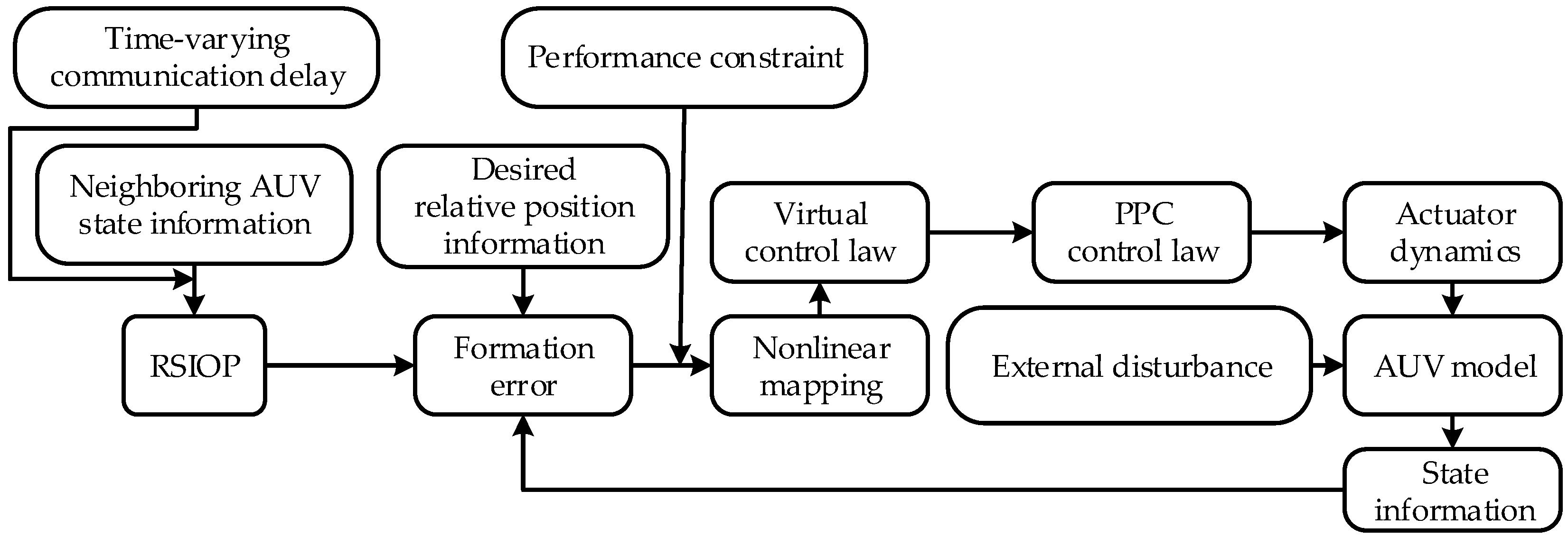
This study is primarily dedicated to designing an adaptive control protocol to enable the formation to achieve a time-varying formation configuration with prescribed performance under conditions of communication delays, external disturbances, and input saturation. Additionally, the formation is guided to follow the desired trajectory generated by the virtual leader. The block diagram of the proposed prescribed performance formation control protocol for the $ith$ AUV is shown in Figure 4.

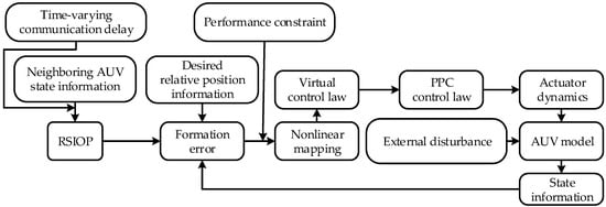
Figure 4. The block diagram of the proposed protocol for formation control.

First, the formation error for the $ith$ AUV is characterized as

$${\gamma }_{e,i}={\displaystyle \sum _{j\in B_i}\left[a_{ij}\left({\eta }_i^{\ast }-{\widehat{\eta }}_j^{\ast }-d_{ij}\right)\right]}$$

(19)

where ${\gamma }_{e,i}={\left[x_{e,i},y_{e,i},z_{e,i}\right]}^T$; $d_{ij}={\left[d_{x,ij},d_{y,ij},d_{z,ij}\right]}^T$ represents the distances between the $ith$ AUV and its neighbors in the x, y, and z directions, respectively, defining the desired formation configuration to be preserved. In order to meet the performance requirements, the formation error must adhere to the following performance function constraints:

$$-{\underset{\_}{\gamma }}_{e,i}\left(t\right)\le {\gamma }_{e,i}\left(t\right)\le {\overline{\gamma }}_{e,i}\left(t\right),t\ge 0$$

(20)

$$\left\{\begin{array}{l}{\overline{\gamma }}_{e,i}\left(t\right)=\left({\overline{\gamma }}_{e,0,i}-{\overline{\gamma }}_{e,\infty ,i}\right)\exp \left(-{\sigma }_{\gamma ,i}t\right)+{\overline{\gamma }}_{e,\infty ,i}\\ {\underset{\_}{\gamma }}_{e,i}\left(t\right)=\left({\underset{\_}{\gamma }}_{e,0,i}-{\underset{\_}{\gamma }}_{e,\infty ,i}\right)\exp \left(-{\sigma }_{\gamma ,i}t\right)+{\underset{\_}{\gamma }}_{e,\infty ,i}\end{array}\right.$$

(21)

where ${\overline{\gamma }}_{e,0,i}$, ${\underset{\_}{\gamma }}_{e,0,i}$, ${\overline{\gamma }}_{e,\infty ,i}$, ${\underset{\_}{\gamma }}_{e,\infty ,i}$, and ${\sigma }_{\gamma ,i}$ are positive constants, with ${\overline{\gamma }}_{e,\infty ,i}\le {\overline{\gamma }}_{e,0,i}$ and ${\underset{\_}{\gamma }}_{e,\infty ,i}\le {\underset{\_}{\gamma }}_{e,0,i}$. As shown in Equations (20) and (21), as $t$ approaches infinity, the formation error will stabilize within the predefined error tolerance $\left[-{\underset{\_}{\gamma }}_{e,\infty ,i},{\overline{\gamma }}_{e,\infty ,i}\right]$.

To guarantee that the errors ${\gamma }_{e,i},\gamma =x,y,z$ adhere to the prescribed performance defined in Equation (21), a mapping function was designed to convert the original constrained tracking errors into an unconstrained form.

$$W_{1,{\gamma }_{e,i}}=f\left({\overline{\gamma }}_{e,i},{\underset{\_}{\gamma }}_{e,i},{\gamma }_{e,i}\right)={\displaystyle \frac{{\overline{\gamma }}_{e,i}{\underset{\_}{\gamma }}_{e,i}{\gamma }_{e,i}}{\left({\overline{\gamma }}_{e,i}-{\gamma }_{e,i}\right)\left({\underset{\_}{\gamma }}_{e,i}+{\gamma }_{e,i}\right)}}$$

(22)

We can observe that $W_{1,{\gamma }_{e,i}}$ will tend toward infinity when the formation error ${\gamma }_{e,i}$ reaches the prescribed bounds. Therefore, if the transformed state $W_{1,{\gamma }_{e,i}}$ stays bounded, the formation tracking errors will adhere to the prescribed performance, as long as the initial states of the control system satisfy the performance constraint specified in Equation (20).

Subsequently, differentiating Equation (22) with respect to time results in

$${\dot{W}}_{1,{\gamma }_{e,i}}=P_{{\gamma }_{e,i}}{\dot{\gamma }}_{e,i}+Q_{{\gamma }_{e,i}}$$

(23)

where $P_{{\gamma }_{e,i}}={\displaystyle \frac{\left({\overline{\gamma }}_{e,i}^2{\underset{\_}{\gamma }}_{e,i}^2+{\overline{\gamma }}_{e,i}{\underset{\_}{\gamma }}_{e,i}{\gamma }_{e,i}^2\right)}{{\left[\left({\overline{\gamma }}_{e,i}-{\gamma }_{e,i}\right)\left({\underset{\_}{\gamma }}_{e,i}+{\gamma }_{e,i}\right)\right]}^2}}, Q_{{\gamma }_{e,i}}={\displaystyle \frac{-\left({\underset{\_}{\gamma }}_{e,i}{\dot{\overline{\gamma }}}_{e,i}+{\dot{\underset{\_}{\gamma }}}_{e,i}{\overline{\gamma }}_{e,i}\right){\gamma }_{e,i}^3-\left({\underset{\_}{\gamma }}_{e,i}^2{\dot{\overline{\gamma }}}_{e,i}-{\overline{\gamma }}_{e,i}^2{\dot{\underset{\_}{\gamma }}}_{e,i}\right){\gamma }_{e,i}^2}{{\left[\left({\overline{\gamma }}_{e,i}-{\gamma }_{e,i}\right)\left({\underset{\_}{\gamma }}_{e,i}+{\gamma }_{e,i}\right)\right]}^2}}$.

4.2. Formation Control Law Design

Step 1. First, define $W_{1,i}={\left[W_{1,x_{e,i}},W_{1,y_{e,i}},W_{1,z_{e,i}}\right]}^T, P_i=diag{\left[P_{x_{e,i}},P_{y_{e,i}},P_{z_{e,i}}\right]}^T$, and $Q_i={\left[Q_{x_{e,i}},Q_{y_{e,i}},Q_{z_{e,i}}\right]}^T$. Subsequently, by combining Equations (4), (19), and (23), the following relationship is obtained:

$${\dot{W}}_{1,i}=P_i{\displaystyle \sum _{j\in B_i}\left[a_{ij}\left(J_{1,i}^{\ast }\left({\eta }_i\right)v_i^{\ast }+J_{2,i}^{\ast }\left({\eta }_i,v_i\right)-J_{1,j}^{\ast }\left({\widehat{\eta }}_j\right){\widehat{v}}_j^{\ast }-J_{2,j}^{\ast }\left({\widehat{\eta }}_j,{\widehat{v}}_j\right)-{\dot{d}}_{ij}\right)\right]}-Q_i$$

(24)

Following the backstepping procedure, the virtual control commands ${\varsigma }_i$ for $v_i^{*}$ are designed as

$$\begin{array}{l}{\varsigma }_i=J_{1,i}^{\ast -1}\left({\eta }_i\right)\left\{P_i^{-1}\left(-{{\rm K}}_{1,i}{W}_{1,i}+Q_i\right)+\right.\\ \hspace{1em}\left.{\displaystyle \sum _{j\in B_i}\left[a_{ij}\left(-J_{2,i}^{\ast }\left({\eta }_i,v_i\right)+J_{1,j}^{\ast }\left({\widehat{\eta }}_j\right){\widehat{v}}_j^{\ast }+J_{2,j}^{\ast }\left({\widehat{\eta }}_j,{\widehat{v}}_j\right)+{\dot{d}}_{ij}\right)\right]}\right\}/b_i\end{array}$$

(25)

where $K_{1,i}\in {ℝ}^{3\times 3}$ is a positive-definite configuration matrix.

Step 2. To address the negative effect of the ‘explosion of complexity’ resulting from differentiating ${\varsigma }_i$, a second-order robust exact differentiator with finite-time convergence capability is introduced [33]. Lemma 2 is given.

$$\left\{\begin{array}{l}{\dot{\varsigma }}_{0,i}=-s_{0,i}{\left|{\varsigma }_{0,i}-{\varsigma }_i\right|}^{{\displaystyle \frac{1}{2}}}sign\left({\varsigma }_{0,i}-{\varsigma }_i\right)+{\varsigma }_{1,i}\\ {\dot{\varsigma }}_{1,i}=-s_{1,i}sign\left({\varsigma }_{1,i}-{\dot{\varsigma }}_{0,i}\right)\end{array}\right.$$

(26)

where $s_{0,i}$ and $s_{1,i}$ are positive design parameters. ${\varsigma }_{0,i}\in {ℝ}^{3\times 3}$ and ${\varsigma }_{1,i}\in {ℝ}^{3\times 3}$, respectively, denote the produce outputs and the outputs of this matrix; moreover, ${\varsigma }_{1,i}$ can be used as a substitute for ${\dot{\varsigma }}_i$.

Lemma 2

([33]). As long as the resulting system is homogeneous and appropriate parameters $s_{0,i}$ and $s_{1,i}$ are selected, this type of robust exact differentiator has finite-time convergence.

Step 3. To achieve additional stability for the virtual control commands, the actual control inputs are crafted as follows:

$$W_{2,i}=v_i^{\ast }-{\varsigma }_{0,i}$$

(27)

$$u_i=-{\alpha }_i^{-1}\left({{\rm K}}_{2,i}{W}_{2,i}-b_i{J}_{1,i}^{\ast T}\left({\eta }_i\right)P_i{W}_{1,i}+C_i^{*}\left(v_i\right)v_i^{*}+D_i^{*}\left(v_i\right)v_i^{*}+g_i^{*}\left({\theta }_i\right)+M_i^{*}{\dot{\varsigma }}_{0,i}\right)$$

(28)

where $W_{2,i}$ denotes the velocity error. $K_{2,i}\in {ℝ}^{3\times 3}$ is a positive-definite designed matrix.

4.3. Stability Analysis

Theorem 1.

For the formation tracking control problem of the AUV model expressed by Equations (1), (2), and (9) obeying Assumption 1 and Assumption 2. If the real-time state information online predictor is designed as in Equation (18), with the virtual control input (25) and control input (28) applied, then under conditions of communication delay, input saturation, and unknown external disturbances, all signals within the closed-loop system will be uniformly ultimately bounded. Moreover, if the initial formation error satisfies condition (20), the prescribed performance can be achieved. This indicates that the AUV formation can follow the target trajectory while maintaining the specified time-varying formation.

Proof of Theorem 1.

The Lyapunov function is defined as follows to demonstrate the asymptotic stability of the closed-loop signals.

$$V={\displaystyle \frac{1}{2}}{\displaystyle \sum _{i=1}^N\left(V_{1,i}^2+V_{2,i}^2\right)}$$

(29)

$$V={\displaystyle \frac{1}{2}}{\displaystyle \sum _{i=1}^N\left(W_{1,i}^T{W}_{1,i}+W_{2,i}^T{M}_i^{\ast }{W}_{2,i}\right)}$$

(30)

Differentiating $V$ with respect to time gives

$$\dot{V}={\displaystyle \sum _{i=1}^N\left(W_{1,i}^T{\dot{W}}_{1,i}+W_{2,i}^T{M}_i^{\ast }{\dot{W}}_{2,i}\right)}$$

(31)

Combining Equations (5), (9), (24), and (25), we further obtain

$$\begin{array}{l}\dot{V}={\displaystyle \sum _{i=1}^N\left[W_{1,i}^T\left(-K_{1,i}{W}_{1,i}+b_i{P}_i{J}_{1,i}^{\ast }\left({\eta }_i\right)W_{2,i}\right)+\right.}\\ \hspace{1em}\left.W_{2,i}^T\left({\alpha }_i{u}_i-{\Omega }_i+o_i+{\Delta }_i^{*}-C_i^{*}\left(v_i\right)v_i^{*}-D_i^{*}\left(v_i\right)v_i^{*}-g_i^{*}\left({\theta }_i\right)-M_i^{*}{\dot{\varsigma }}_{0,i}\right)\right]\end{array}$$

(32)

Substituting the control input from Equation (28), we obtain:

$$\dot{V}={\displaystyle \sum _{i=1}^N\left(-K_{1,i}{W}_{1,i}^T{W}_{1,i}-K_{2,i}{W}_{2,i}^T{W}_{2,i}-W_{2,i}^T\left(-{\Omega }_i+o_i+{\Delta }_i^{*}\right)\right)}$$

(33)

$$\dot{V}\le {\displaystyle \sum _{i=1}^N\left(-K_{1,i}{‖W_{1,i}‖}^2-K_{2,i}{‖W_{2,i}‖}^2+‖W_{2,i}‖‖{\Omega }_i‖+‖W_{2,i}‖‖o_i+{\Delta }_i^{*}‖\right)}$$

(34)

$$\dot{V}\le {\displaystyle \sum _{i=1}^N\left(-K_{1,i}{‖W_{1,i}‖}^2-‖W_{2,i}‖\left(K_{2,i}‖W_{2,i}‖-{ƛ}_i\right)\right)}$$

(35)

$${ƛ}_i=‖{\Omega }_i‖+‖o_i+{\Delta }_i^{*}‖$$

(36)

Based on Assumption 2 and the discussion below Equation (9), it can be concluded that

$${\displaystyle \sum _{i=1}^N{ƛ}_i}={\displaystyle \sum _{i=1}^N\left(‖{\Omega }_i‖+‖o_i+{\Delta }_i^{*}‖\right)}<a_i$$

(37)

$$\dot{V}\le {\displaystyle \sum _{i=1}^N\left(-K_{1,i}{‖W_{1,i}‖}^2-‖W_{2,i}‖{\overline{a}}_i\right)}$$

(38)

where ${\overline{a}}_i=K_{2,i}‖W_{2,i}‖-a_i$; one further has $\dot{V}<0\left(or {\overline{a}}_i>0\right)$ as long as $‖W_{2,i}‖>{\mathit{\Gamma }}_i$

$${\mathit{\Gamma }}_i={\displaystyle \frac{{\overline{a}}_i}{K_{2,i}}}$$

(39)

After calculations, the final result is obtained as

$$V\le {\displaystyle \frac{1}{2}}{\displaystyle \sum _{i=1}^N\left({\mathit{\Gamma }}_{1,i}^2+{\mathit{\Gamma }}_{2,i}^2\right)}$$

(40)

$${\Gamma }_{1,i}=\max \left({\displaystyle \frac{b_i‖P_i‖‖J_{1,i}^{\ast }\left({\eta }_i\right)‖‖{\Gamma }_{2,i}‖}{K_{1,i}}},\sqrt{{\displaystyle \frac{2V_{1,i}\left(0\right)}{{\mathsf{{\rm Y}}}_{1,i}}}}\right), {\Gamma }_{2,i}=\max \left({\displaystyle \frac{{\overline{a}}_i}{K_{2,i}}},\sqrt{{\displaystyle \frac{2V_{2,i}\left(0\right)}{{\mathsf{{\rm Y}}}_{2,i}}}}\right)$$

(41)

$$‖W_{1,i}‖\le {\Gamma }_{1,i}, ‖W_{2,i}‖\le {\Gamma }_{2,i}$$

(42)

where ${\mathsf{{\rm Y}}}_{1,i}$ and ${\mathsf{{\rm Y}}}_{2,i}$ are appropriate positive constants. From the above conclusions, we obtain that $V$ is bounded as time approaches infinity, ensuring that all signals within the closed-loop system are kept bounded. More importantly, the boundedness of the mapped system states that $W_{1,i}$ is also ensured. From the analysis following Equation (22), it can be concluded that the prescribed performance of the formation can be attained under the proposed protocol. Therefore, Theorem 1 is proven. □

Remark 1.

The proof demonstrates that by keeping the transformed errors $W_{1,i}$ and $W_{2,i}$ bounded, the closed-loop system can achieve the prescribed performance stability. This indicates that the proposed control protocol can achieve its objectives without reducing $W_{1,i}$ and $W_{2,i}$ to arbitrarily small regions. Following this logic, as described in reference [34], the uncertainty disturbance ${ƛ}_i$ can be compensated even without any auxiliary control signals, as it only affects the magnitude of $W_{1,i}$ and $W_{2,i}$ but does not alter the achieved stability properties. Separating the tracking performance from the uncertainty disturbances significantly enhances the robustness of the proposed control protocol.

5. Simulation Results

In this section, the proposed control protocol’s effectiveness is evaluated through a series of simulation tests. All simulations in this study were performed using MATLAB R2023a on a personal computer running Windows 10, equipped with an Intel Core i7-8750H processor (2.20 GHz) and 16 GB of RAM.

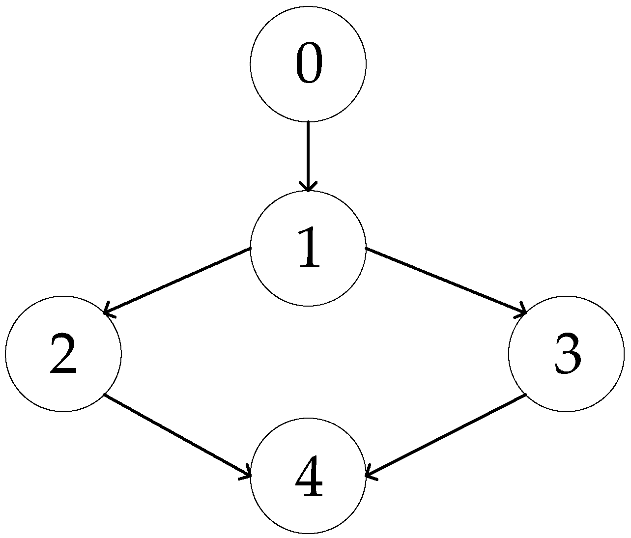
The study focuses on an AUV formation, which includes a virtual leader and four underactuated AUVs. Assume that the trajectory of the virtual leader is already loaded onto AUV1, meaning that there is no communication delay between them. The main physical parameters and partial hydrodynamic coefficients of the AUVs were measured experimentally and are tabulated in Table 1 and Table 2. Additionally, the communication topology is shown in Figure 5, with the virtual leader designated as number 0.

Table 1. Main physical parameters of the AUVs.

Parameters	Value	Parameters	Value
$m_i$	$183 \mathrm{Kg}$	$L_i$	2.55 $\mathrm{M}$
$G{M}_{L,i}$	$0.0217 \mathrm{M}$	${\rho }_i$	$1024 \mathrm{Kg}/{\mathrm{m}}^3$
Maximum thrust	$100 \mathrm{N}$	Maximum Horizontal/Vertical Rudder Force	$25/50 \mathrm{N}\cdot \mathrm{m}$

Table 2. Partial hydrodynamic coefficients of the AUVs.

Parameters	Value	Parameters	Value
$m_{11,i}$	$188 \mathrm{Kg}$	$m_{22,i}$	$263 \mathrm{Kg}$
$m_{33,i}$	$263 \mathrm{Kg}$	$m_{44,i}$	$271 {\mathrm{Kgm}}^2$
$m_{55,i}$	$271 {\mathrm{Kgm}}^2$	$X_{u,i}$	$16.65\left|v{u}_i\right| \mathrm{Kg}/\mathrm{s}$
$Y_{v,i}$	$149.68\left|v{u}_i\right| \mathrm{Kg}/\mathrm{s}$	$Z_{w,i}$	$142.23\left|v{u}_i\right| \mathrm{Kg}/\mathrm{s}$
$M_{q,i}$	$220.92\left|v{u}_i\right| \mathrm{Kg}/\mathrm{s}$	$N_{r,i}$	$252.83\left|v{u}_i\right| \mathrm{Kg}/\mathrm{s}$

Figure 5. The communication topology graph.

The virtual leader’s trajectory is defined as $\left[\left(50\cos (0.01t)-50+50\sin (0.02t)\right)\right.$${\left.\mathrm{m},\left(50\sin (0.01t)+50\cos (0.02t)-50\right)\mathrm{m},\left(-0.1t\right)\mathrm{m}\right]}^T$. The initial position information, velocity information, and the desired relative position information between neighboring AUVs are shown in Table 3.

Table 3. Formation state information settings.

Parameters	Value
${\eta }_1\left(0\right)$	${\left[-1.35\mathrm{m},1\mathrm{m},-1\mathrm{m},0\mathrm{rad},0\mathrm{rad}\right]}^T$
${\eta }_2\left(0\right)$	$\left[-8.75\mathrm{m},-7\mathrm{m}\right.,{\left.-2\mathrm{m},0\mathrm{rad},0\mathrm{rad}\right]}^T$
${\eta }_3\left(0\right)$	${\left[6.75\mathrm{m},-7\mathrm{m},-3\mathrm{m},0\mathrm{rad},0\mathrm{rad}\right]}^T$
${\eta }_4\left(0\right)$	$\left[-2.35\mathrm{m},-15.5\right.\mathrm{m},-2{\left.\mathrm{m},0\mathrm{rad},0\mathrm{rad}\right]}^T$
$v_i\left(0\right)$	$\left[0\mathrm{m}/\mathrm{s},0\mathrm{m}/\mathrm{s},0\mathrm{m}/\mathrm{s}\right.,{\left.0\mathrm{rad}/\mathrm{s},0\mathrm{rad}/\mathrm{s}\right]}^T$
$d_{10}$	${\left[0\mathrm{m},0\mathrm{m},0\mathrm{m}\right]}^T$
$d_{21}$	$\left[-10\mathrm{m},\right.(-5\cos \left({\displaystyle \frac{\pi }{300}}\mathrm{t}\right){\left.\left.-5\right)\mathrm{m},\left(-0.5\cos \left({\displaystyle \frac{\pi }{300}}\mathrm{t}\right)-1.5\right)\mathrm{m}\right]}^T$
$d_{31}$	${\left[10\mathrm{m},\left(-5\cos \left({\displaystyle \frac{\pi }{300}}\mathrm{t}\right)-5\right)\mathrm{m},\left(-1.5\cos \left({\displaystyle \frac{\pi }{300}}\mathrm{t}\right)+0.5\right)\mathrm{m}\right]}^T$
$d_{42}$	${\left[8\mathrm{m},\left(-8\cos \left({\displaystyle \frac{\pi }{1200}}\mathrm{t}\right)\right)\mathrm{m},\left(-1.5\cos \left({\displaystyle \frac{\pi }{300}}\mathrm{t}\right)+1\right)\mathrm{m}\right]}^T$
$d_{43}$	${\left[-8\mathrm{m},\left(-8\cos \left({\displaystyle \frac{\pi }{1200}}\mathrm{t}\right)\right)\mathrm{m},\left(-1.5\cos \left({\displaystyle \frac{\pi }{300}}\mathrm{t}\right)+2\right)\mathrm{m}\right]}^T$

The communication delays between AUVs are set as ${\tau }_{21}={\tau }_{31}=\left(2-0.25\cos \left({\displaystyle \frac{\pi }{600}}t\right)\right)\mathrm{s}$,${\tau }_{42}={\tau }_{43}=\left(1.5+0.25\cos \left({\displaystyle \frac{\pi }{600}}t\right)\right)\mathrm{s}$. The external ocean current disturbances are defined as ${\Delta }_i=\left[\left(1.3+2\sin \left({\displaystyle \frac{\pi }{50}}\mathrm{t}\right)\right)\mathrm{N},\left(-0.9+2\sin \left({\displaystyle \frac{\pi }{50}}\mathrm{t}\right)\right)\mathrm{N},\left(0.5\cos \left({\displaystyle \frac{\pi }{10}}\mathrm{t}\right)\right)\mathrm{N},\left(\cos \left({\displaystyle \frac{\pi }{10}}\mathrm{t}\right)\right)\mathrm{N}\cdot \mathrm{m},\left(-\sin \left({\displaystyle \frac{\pi }{50}}\mathrm{t}+{\displaystyle \frac{\pi }{3}}\right)\right.\right.$${\left.\left.-4\sin \left({\displaystyle \frac{\pi }{100}}\mathrm{t}\right)\right)\mathrm{N}\cdot \mathrm{m}\right]}^T$. The values of the actuator dynamics model are set as described below Figure 2. Additionally, Table 4 presents the main control parameters used in the simulation experiment. All parameters were selected empirically within the range that ensures the stability of all closed-loop system signals, as determined by the stability analysis. Following this, a systematic tuning process was implemented, during which the control gains were iteratively adjusted to find the optimal balance between robustness and responsiveness, ultimately leading to a well-founded and effective determination of the parameters.

Table 4. Key control parameters of the AUVs.

Parameters	Value
${\left[{\overline{\gamma }}_{e,0,i},{\underset{\_}{\gamma }}_{e,0,i}\right]}^T$	${\left[5.1,1.1\right]}^T$$, \mathrm{if} {\gamma }_{e,i}\left(0\right)>0$${\left[1.1,5.1\right]}^T$, else
${\left[{\overline{\gamma }}_{e,\infty ,i},{\underset{\_}{\gamma }}_{e,\infty ,i}\right]}^T$	${\left[0.1,0.1\right]}^T$
${\left[c_{\rho ,ij,1},c_{\rho ,ij,2}\right]}^T$	${\left[0.8,0.1\right]}^T$
${\left[s_{0,i},s_{1,i}\right]}^T$	${\left[1,0.1\right]}^T$
${\left[K_{1,i},K_{2,i}\right]}^T$	${\left[0.2,0.1,0.1\right]}^T, {\left[200,200,400\right]}^T$

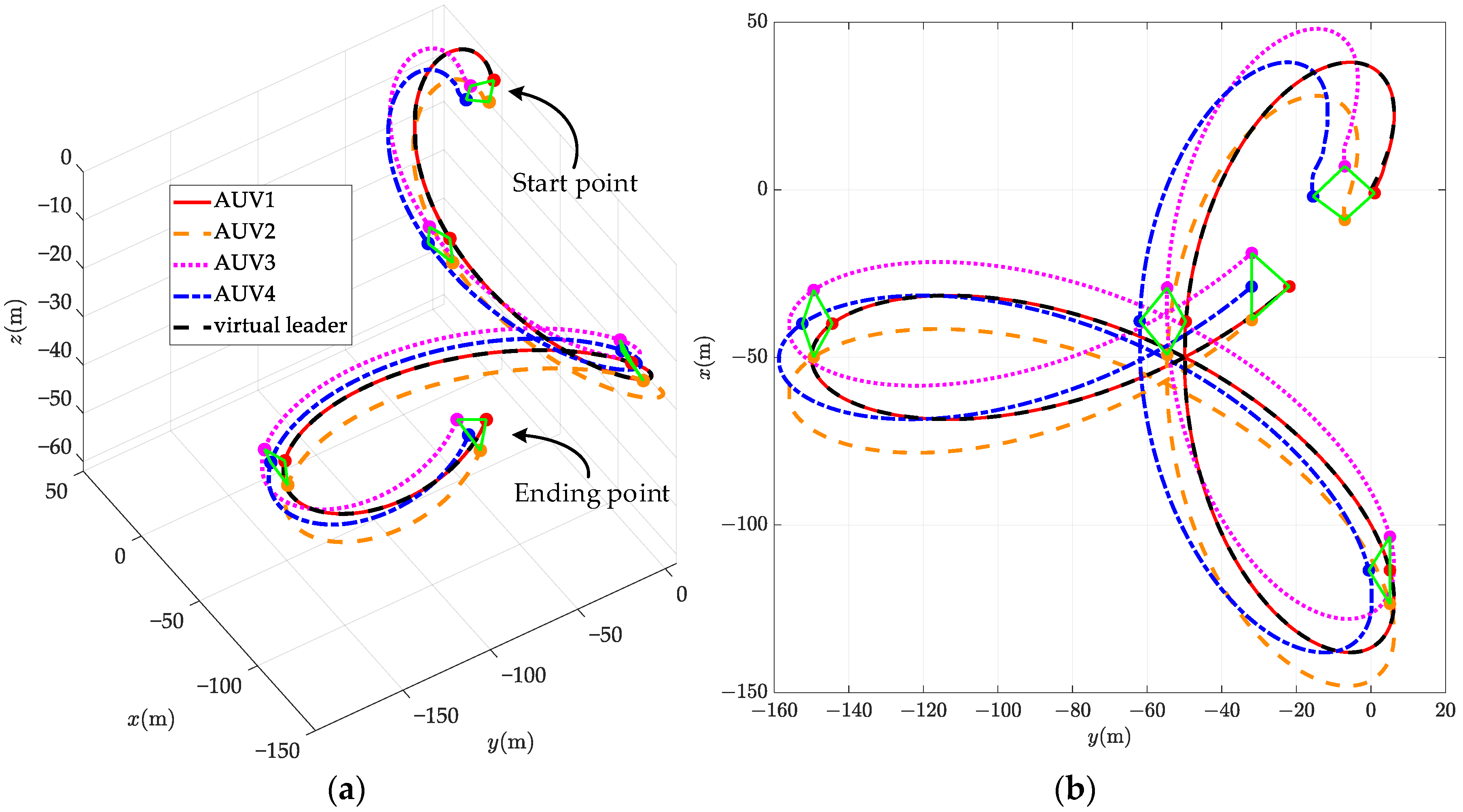
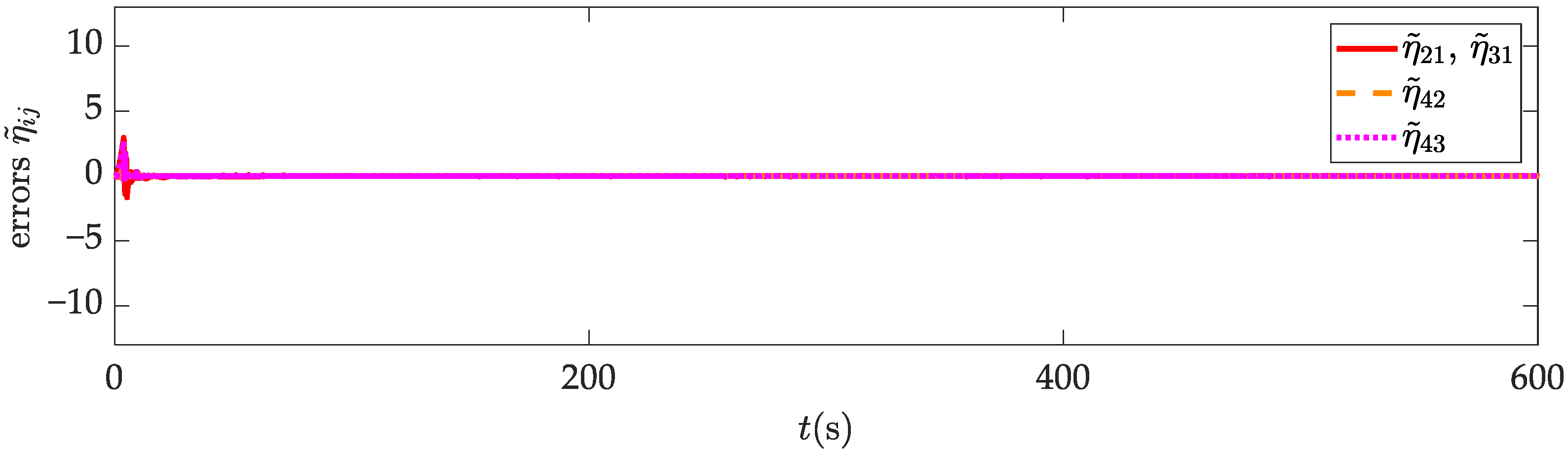
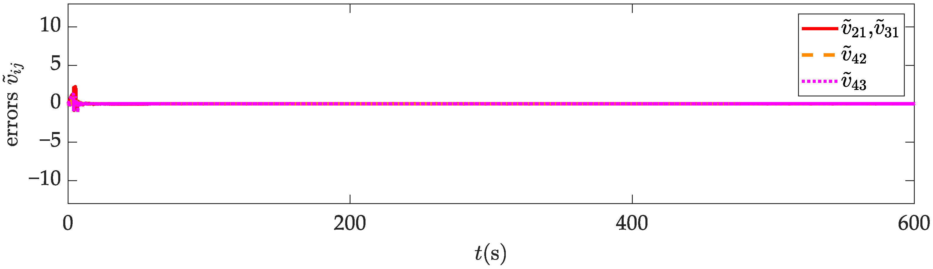
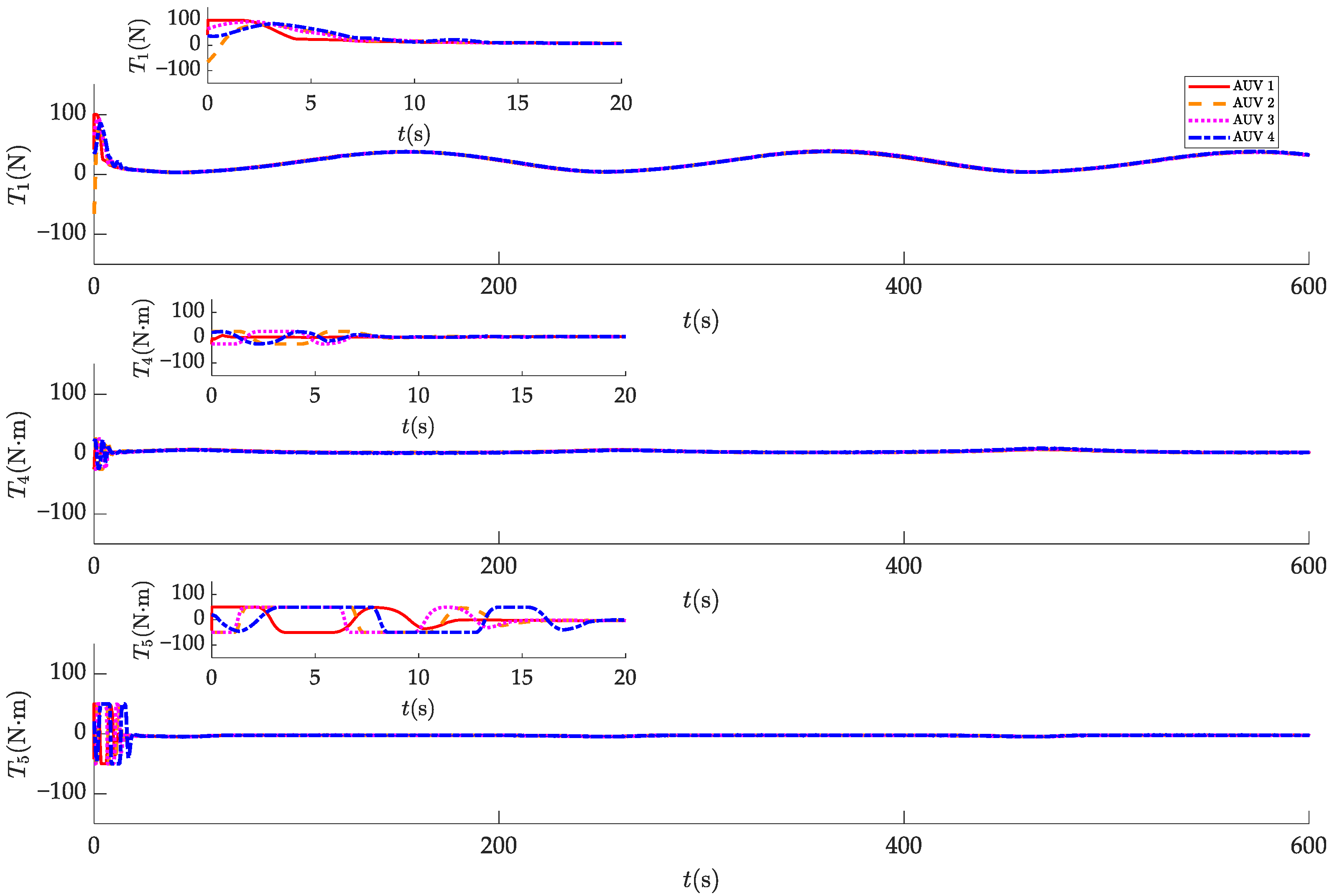
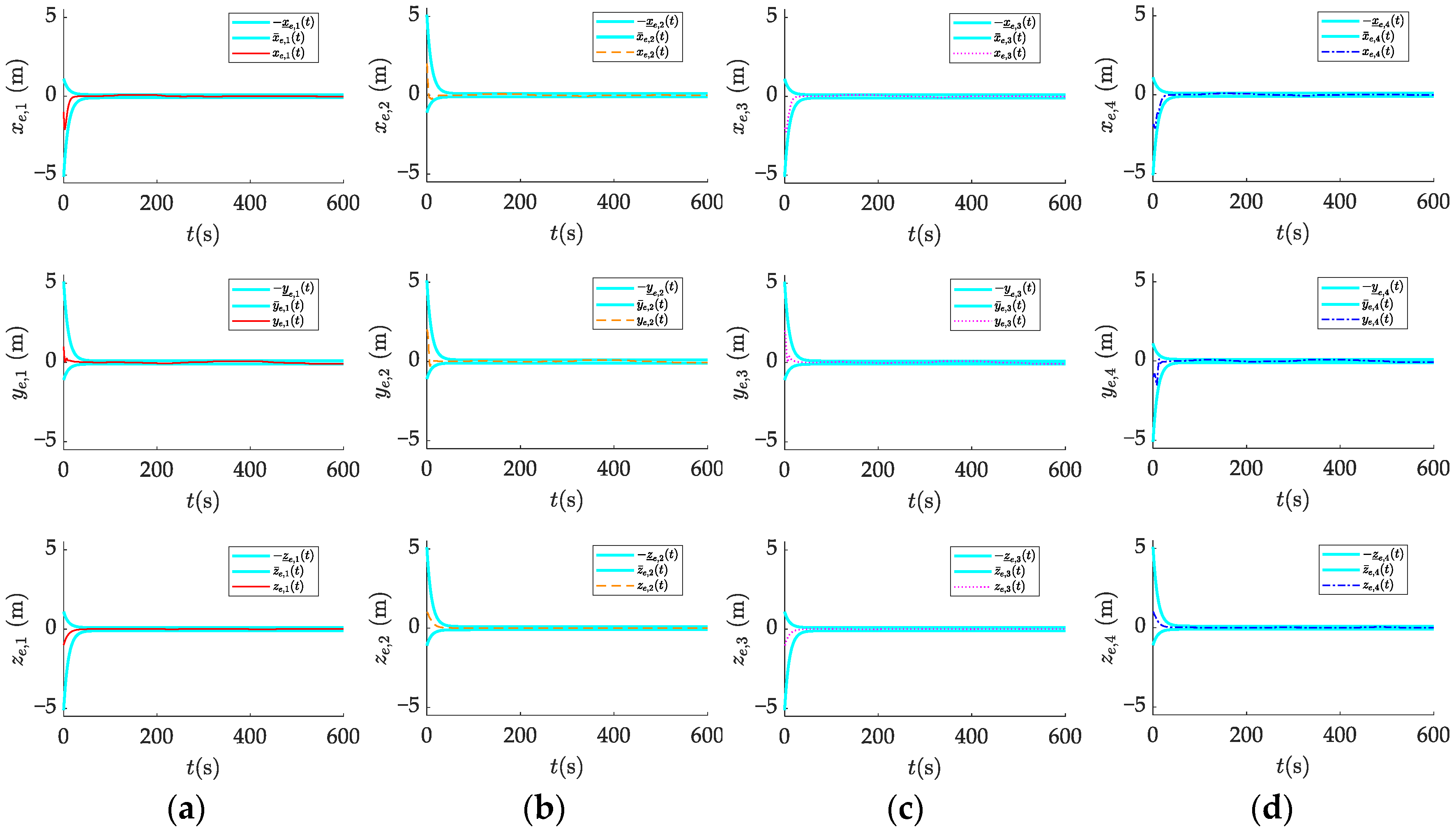
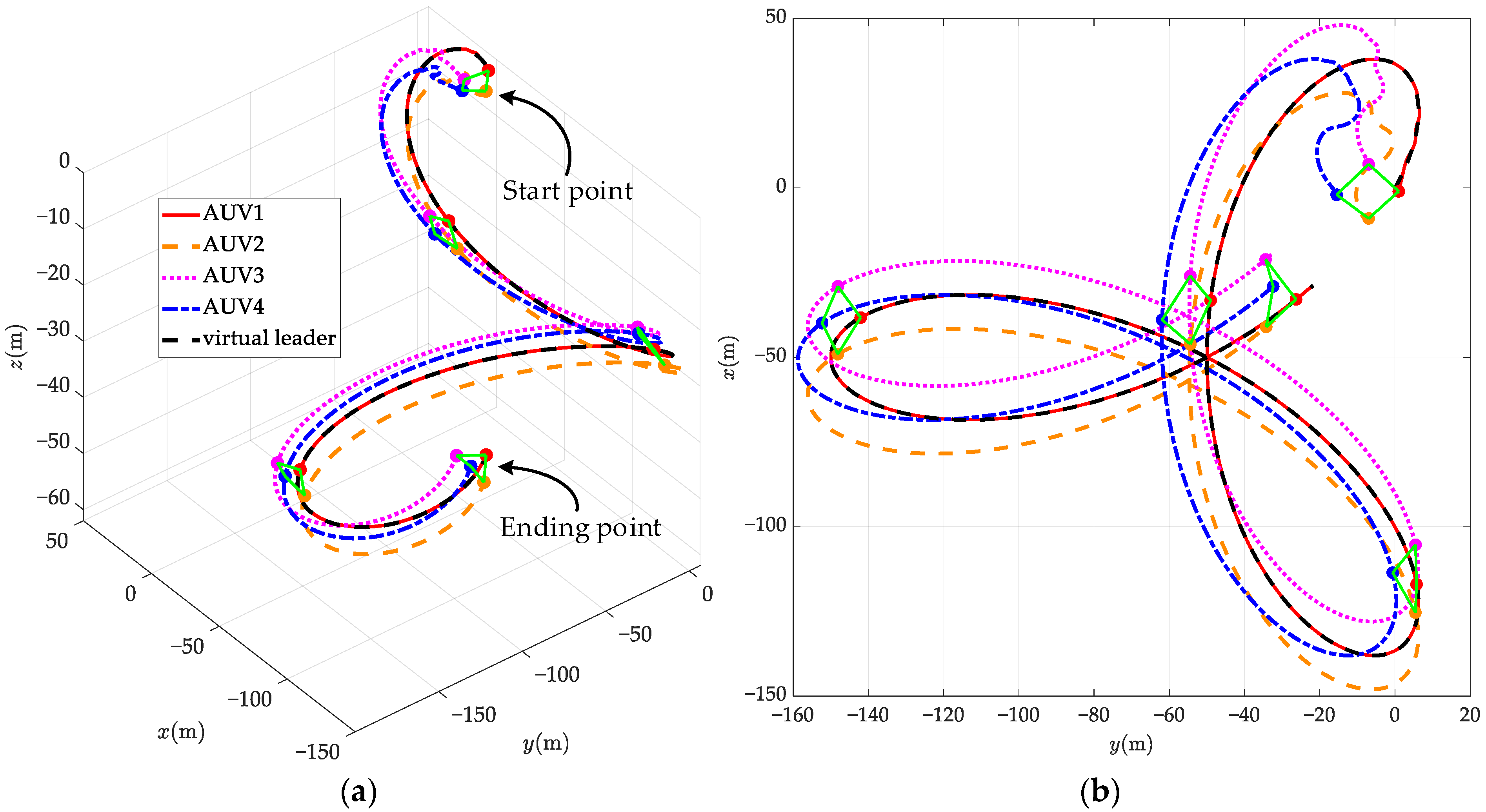
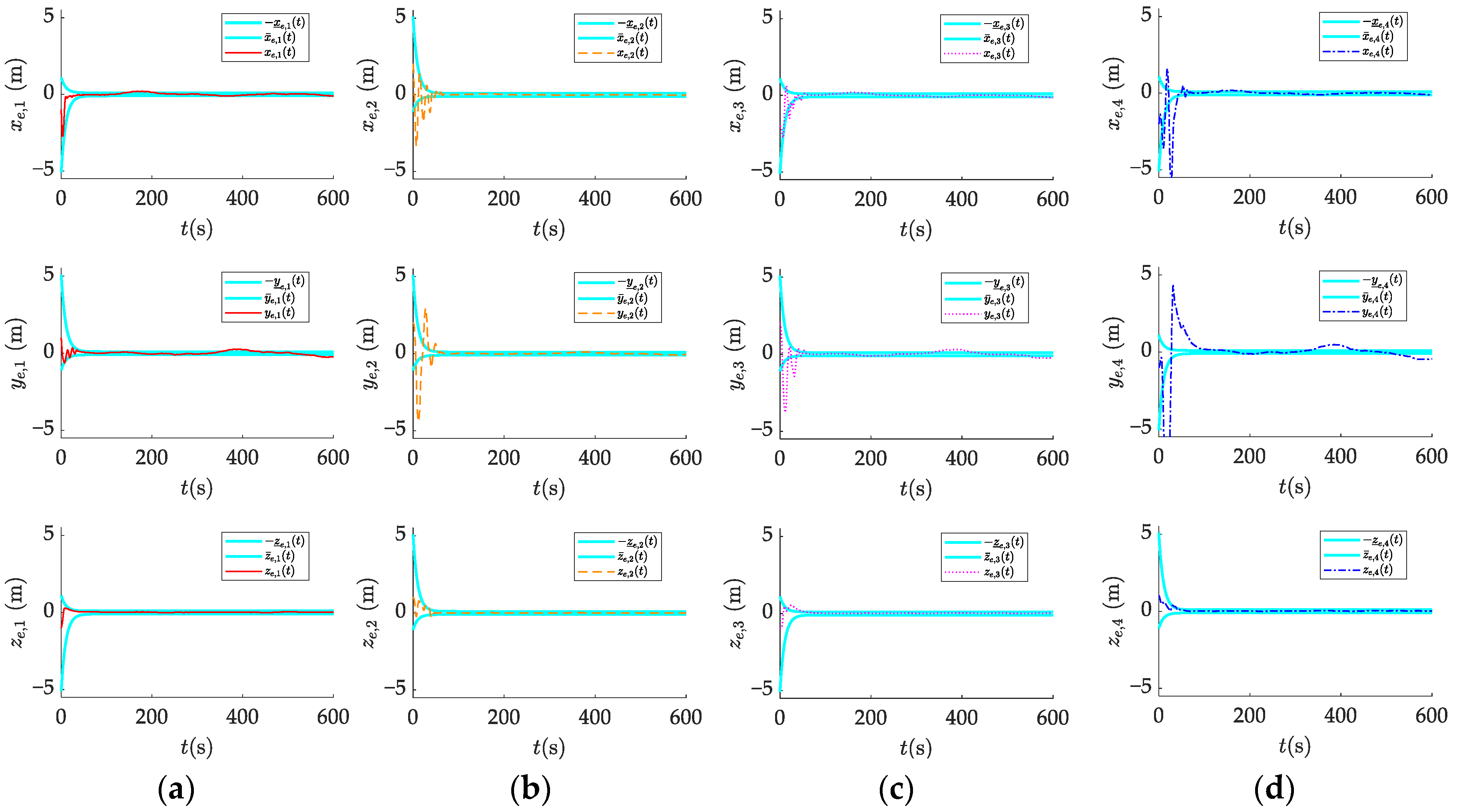
The simulation outcomes of the proposed control protocol are presented in Figure 6, Figure 7, Figure 8, Figure 9 and Figure 10. The trajectories of the AUV formation are shown in Figure 6, demonstrating that the AUVs successfully follow the desired trajectory. The formation configuration transitions from a quadrilateral to a triangle, achieving the predetermined formation transformation. The position state information prediction errors ${\tilde{\eta }}_j\left(t\right)$ and the velocity state information prediction errors ${\tilde{v}}_j\left(t\right)$ of the AUV formation are illustrated in Figure 7 and Figure 8, respectively. In the legend, ${\tilde{\eta }}_{ij}$ and ${\tilde{v}}_{ij}$ represent the estimates of the state information of the $ith$ AUV for the $jth$ AUV. All state estimation errors converge within approximately 10 s. These results indicate that the RSIOP can accurately and quickly estimate the current state information ${\Phi }_j\left(t\right)$ of neighboring AUVs considering communication delays, thereby ensuring the accuracy and stability of formation control. Observing the actual control inputs of the AUV formation in Figure 9, we can conclude that the saturation constraints are not violated under the dead-zone model. Additionally, all actual control input curves are smooth, with no significant oscillations, aligning with the actuator’s executable capability in practical scenarios. The formation error response, shown in Figure 10, indicates that the AUV formation can achieve the prescribed performance with the designed control protocol. In other words, both the transient- and steady-state performance of the formation are ensured. The formation errors converge within 16 s and remain within the performance constraint bounds. Moreover, the steady-state formation control error for each AUV in the x, y, and z directions is less than 0.1 m Furthermore, it can be clearly observed that external uncertainty disturbances and input saturation have minimal impact on the formation control accuracy, indicating that the proposed control protocol exhibits good robustness. Thus, the validity of Theorem 1 is verified.

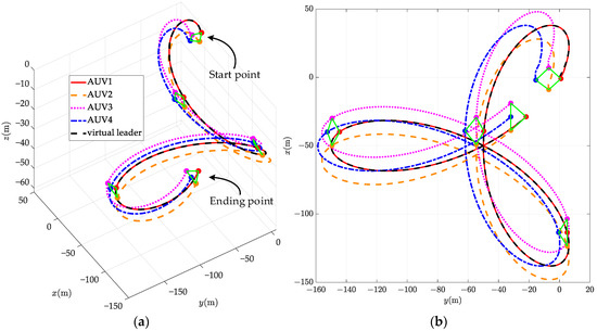
Figure 6. Motion trajectories of the AUV formation in (a) x–y–z plane; (b) x–y plane.

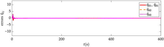
Figure 7. Position state information prediction error in AUV formation.

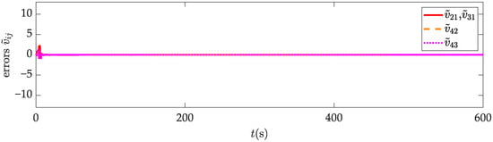
Figure 8. Velocity state information prediction error in AUV formation.

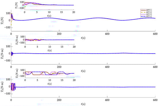
Figure 9. Actual control inputs of the AUV formation.

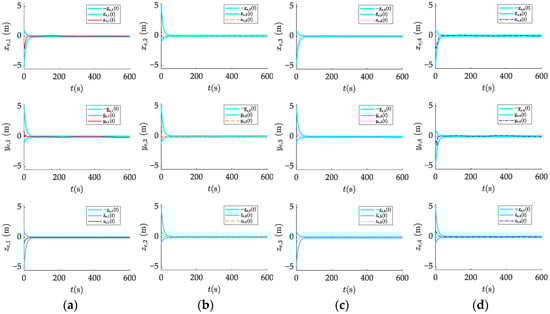
Figure 10. Formation error responses of (a) AUV1, (b) AUV2, (c) AUV3, and (d) AUV4.

To validate the effectiveness of the designed control protocol, the simulation results of the proposed method were compared against those obtained from simulation tests using the traditional backstepping control protocol. Additionally, during the simulations, the designed RSIOP was not used to compensate for delayed state information. The simulation conditions were kept entirely consistent with those in the previous simulations. The results of the simulations are as follows:

Figure 11 shows the movement trajectories of the AUV formation under the traditional backstepping control method. It is evident that, under the condition of not considering the solution to communication delays, the control accuracy of the formation cannot be guaranteed, and the AUV formation cannot form the predetermined formation structure, thus failing to complete the mission objectives. Figure 12 shows the formation error response under the traditional backstepping control method. It can be concluded that the formation error needs to be reduced to within approximately 100 s and cannot be maintained within the performance constraint bounds proposed in this paper, resulting in a significant decrease in control performance. To further quantify the control accuracy differences between the two methods used in this study, we introduce integrated absolute error (IAE), which is expressed as $\mathrm{IAE}\left({\gamma }_{e,i}\right)={\displaystyle \sum _{i=1}^N{\displaystyle {\int }_0^t‖{\gamma }_{e,i}‖} dt}$, with ${\gamma }_{e,i}=x_{e,i},y_{e,i},z_{e,i}$. The maximum instantaneous formation error change is formulated as $\max \left({\gamma }_{e,i}\right)=\max \left({\displaystyle \sum _{i=1}^N‖{\gamma }_{e,i}‖}\right)$. The analysis results, as shown in Table 5, indicate that the control protocol proposed in this paper has superior control accuracy.

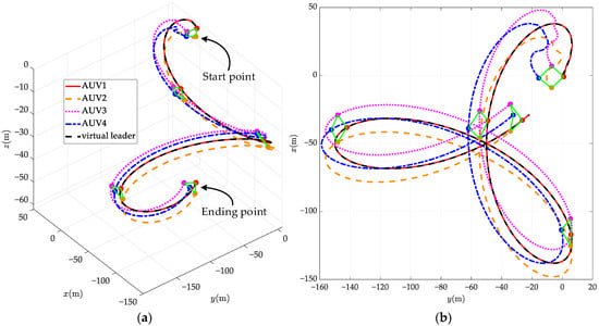
Figure 11. Motion trajectories of the AUV formation under the traditional backstepping control method in (a) x–y–z plane; (b) x–y plane.

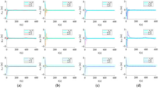
Figure 12. Formation error responses under the traditional backstepping control method of (a) AUV1, (b) AUV2, (c) AUV3, and (d) AUV4.

Table 5. The IAE values of the two control methods.

Parameters	$\mathbf{IAE}\left({\mathit{x}}_{\mathit{e},\mathit{i}}\right)$	$\mathbf{IAE}\left({\mathit{y}}_{\mathit{e},\mathit{i}}\right)$	$\mathbf{IAE}\left({\mathit{z}}_{\mathit{e},\mathit{i}}\right)$	$\mathbf{max}\left({\mathit{x}}_{\mathit{e},\mathit{i}}\right)$	$\mathbf{max}\left({\mathit{y}}_{\mathit{e},\mathit{i}}\right)$	$\mathbf{max}\left({\mathit{z}}_{\mathit{e},\mathit{i}}\right)$
The proposed protocol	1237.49	1252.75	612.64	7.43	6	4
Backstepping method	2989	5646.97	1056.65	9.66	15.61	4

Remark 2.

The traditional backstepping method was chosen for comparison in this section, rather than simply omitting the RSIOP, because without the state compensation provided by the RSIOP under conditions of communication delays, the proposed prescribed performance control protocol would not achieve convergence of the formation error. This phenomenon further underscores the necessity and effectiveness of developing the RSIOP.

Although this paper has effectively addressed the issue of formation control under time-varying communication delays, there are still some limitations. One of the key limitations of the proposed formation control protocol with prescribed performance is that it requires the initial formation error of the AUVs to be within the performance constraint bounds. Moreover, the final value must be reasonably determined based on the AUVs’ performance capabilities, as determined through experience. If these conditions are not met, the convergence of the formation control errors cannot be guaranteed. This is an area that requires further investigation, particularly in developing strategies for handling cases where the initial errors exceed the prescribed bounds. In addition, the application of the real-time state information online predictor (RSIOP) and the prescribed performance control (PPC) framework does involve certain computational complexities. In dynamic environments, the algorithm must quickly adapt to changes in communication delays and external disturbances. As the number of AUVs in the formation increases, this will inevitably increase the computational burden. Ensuring that these computations can be performed in real-time without causing delays in the control response is also a significant challenge. To address this, we have already made some trade-offs at the algorithm level. While the algorithm aims to maintain high accuracy in state prediction and control actions, some approximations have been made to reduce the computational load. Furthermore, we will explore the use of parallel computing techniques and hardware acceleration to enhance the real-time performance of the algorithm in future work, especially in more complex and dynamic scenarios.

6. Conclusions

In this brief, a distributed prescribed performance tracking control protocol is proposed for underactuated AUV formation systems under time-varying communication delays, which are constrained by external uncertainties and input saturation. The formation system is required to achieve the specified formation configuration transformation while also tracking the desired trajectory as a whole.

First, a delayed state information compensation method-based RSIOP is proposed to mitigate the adverse effects of acoustic communication delays on formation control. Second, a formation control protocol is developed by combining backstepping technology and nonlinear mapping methods, taking into account external uncertainties, input saturation, and predefined performance constraints during the design process. Furthermore, the stability of the closed-loop system is established using the Lyapunov method. Lastly, simulation results confirm the robustness and effectiveness of the proposed protocol.

In future work, we plan to consider more practical scenarios and further investigate the limitations of the proposed protocol, such as computational complexity and sensitivity to initial conditions. Additionally, we intend to validate the practicality of our algorithm through experimental testing.

References

- Xie, T.; Li, Y.; Jiang, Y.; Pang, S.; Wu, H. Turning Circle Based Trajectory Planning Method of an Underactuated AUV for the Mobile Docking Mission. Ocean Eng. 2021, 236, 109546. [Google Scholar] [CrossRef]
- Wang, C.; Cai, W.; Lu, J.; Ding, X.; Yang, J. Design, Modeling, Control, and Experiments for Multiple AUVs Formation. IEEE Trans. Autom. Sci. Eng. 2022, 19, 2776–2787. [Google Scholar] [CrossRef]
- Li, B.; Wen, G.; Peng, Z.; Huang, T.; Rahmani, A. Fully Distributed Consensus Tracking of Stochastic Nonlinear Multiagent Systems With Markovian Switching Topologies via Intermittent Control. IEEE Trans. Syst. Man Cybern. Syst. 2022, 52, 3200–3209. [Google Scholar] [CrossRef]
- Qiao, L.; Zhang, W. Trajectory Tracking Control of AUVs via Adaptive Fast Nonsingular Integral Terminal Sliding Mode Control. IEEE Trans. Ind. Inform. 2020, 16, 1248–1258. [Google Scholar] [CrossRef]
- Vu, M.T.; Le Thanh, H.N.N.; Huynh, T.-T.; Thang, Q.; Duc, T.; Hoang, Q.-D.; Le, T.-H. Station-Keeping Control of a Hovering Over-Actuated Autonomous Underwater Vehicle Under Ocean Current Effects and Model Uncertainties in Horizontal Plane. IEEE Access 2021, 9, 6855–6867. [Google Scholar] [CrossRef]
- Zhou, Z.; Liu, J.; Yu, J. A Survey of Underwater Multi-Robot Systems. IEEE/CAA J. Autom. Sin. 2022, 9, 1–18. [Google Scholar] [CrossRef]
- Liu, Y.; Liu, J.; He, Z.; Li, Z.; Zhang, Q.; Ding, Z. A Survey of Multi-Agent Systems on Distributed Formation Control. Unmanned Syst. 2023, 12, 913–926. [Google Scholar] [CrossRef]
- Li, D.; Du, L. AUV Trajectory Tracking Models and Control Strategies: A Review. J. Mar. Sci. Eng. 2021, 9, 1020. [Google Scholar] [CrossRef]
- Wang, J.; Dong, H.; Chen, F.; Vu, M.T.; Shakibjoo, A.D.; Mohammadzadeh, A. Formation Control of Non-Holonomic Mobile Robots: Predictive Data-Driven Fuzzy Compensator. Mathematics 2023, 11, 1804. [Google Scholar] [CrossRef]
- Yan, T.; Xu, Z.; Yang, S.X. Consensus Formation Tracking for Multiple AUV Systems Using Distributed Bioinspired Sliding Mode Control. IEEE Trans. Intell. Veh. 2023, 8, 1081–1092. [Google Scholar] [CrossRef]
- Chen, B.; Hu, J.; Zhao, Y.; Ghosh, B.K. Finite-Time Velocity-Free Rendezvous Control of Multiple AUV Systems With Intermittent Communication. IEEE Trans. Syst. Man Cybern. Syst. 2022, 52, 6618–6629. [Google Scholar] [CrossRef]
- Hadi, B.; Khosravi, A.; Sarhadi, P. A Review of the Path Planning and Formation Control for Multiple Autonomous Underwater Vehicles. J. Intell. Robot. Syst. 2021, 101, 67. [Google Scholar] [CrossRef]
- Yang, Y.; Xiao, Y.; Li, T. A Survey of Autonomous Underwater Vehicle Formation: Performance, Formation Control, and Communication Capability. IEEE Commun. Surv. Tutor. 2021, 23, 815–841. [Google Scholar] [CrossRef]
- Yan, Z.; Zhang, C.; Tian, W.; Zhang, M. Formation Trajectory Tracking Control of Discrete-Time Multi-AUV in a Weak Communication Environment. Ocean Eng. 2022, 245, 110495. [Google Scholar] [CrossRef]
- Li, J.; Zhang, H.; Chen, T.; Wang, J. AUV Formation Coordination Control Based on Transformed Topology under Time-Varying Delay and Communication Interruption. J. Mar. Sci. Eng. 2022, 10, 950. [Google Scholar] [CrossRef]
- Li, J.; Tian, Z.; Zhang, H. Discrete-Time AUV Formation Control with Leader-Following Consensus under Time-Varying Delays. Ocean Eng. 2023, 286, 115678. [Google Scholar] [CrossRef]
- Zhang, W. Leader-Following Consensus of Discrete-Time Multi-AUV Recovery System with Time-Varying Delay. Ocean Eng. 2021, 219, 108258. [Google Scholar] [CrossRef]
- Zeng, Z.; Yu, H.; Guo, C.; Yan, Z. Finite-Time Coordinated Formation Control of Discrete-Time Multi-AUV with Input Saturation under Alterable Weighted Topology and Time-Varying Delay. Ocean Eng. 2022, 266, 112881. [Google Scholar] [CrossRef]
- Yan, Z.; Yang, Z.; Pan, X.; Zhou, J.; Wu, D. Virtual Leader Based Path Tracking Control for Multi-UUV Considering Sampled-Data Delays and Packet Losses. Ocean Eng. 2020, 216, 108065. [Google Scholar] [CrossRef]
- Li, L.; Li, Y.; Zhang, Y.; Xu, G.; Zeng, J.; Feng, X. Formation Control of Multiple Autonomous Underwater Vehicles under Communication Delay, Packet Discreteness and Dropout. J. Mar. Sci. Eng. 2022, 10, 920. [Google Scholar] [CrossRef]
- Du, J.; Li, J.; Lewis, F.L. Distributed 3-D Time-Varying Formation Control of Underactuated AUVs With Communication Delays Based on Data-Driven State Predictor. IEEE Trans. Ind. Inform. 2023, 19, 6963–6971. [Google Scholar] [CrossRef]
- Bechlioulis, C.P.; Rovithakis, G.A. Robust Adaptive Control of Feedback Linearizable MIMO Nonlinear Systems With Prescribed Performance. IEEE Trans. Autom. Control 2008, 53, 2090–2099. [Google Scholar] [CrossRef]
- Liu, X.; Zhang, M.; Wang, S. Adaptive Region Tracking Control with Prescribed Transient Performance for Autonomous Underwater Vehicle with Thruster Fault. Ocean Eng. 2020, 196, 106804. [Google Scholar] [CrossRef]
- Sun, Y.; Liu, M.; Qin, H.; Wang, H.; Ding, Z. Full Prescribed Performance Trajectory Tracking Control Strategy of Autonomous Underwater Vehicle with Disturbance Observer. ISA Trans. 2024, 151, 117–130. [Google Scholar] [CrossRef]
- Huang, B.; Zhou, B.; Zhang, S.; Zhu, C. Adaptive Prescribed Performance Tracking Control for Underactuated Autonomous Underwater Vehicles with Input Quantization. Ocean Eng. 2021, 221, 108549. [Google Scholar] [CrossRef]
- Wei, C.; Chen, Q.; Liu, J.; Yin, Z.; Luo, J. An Overview of Prescribed Performance Control and Its Application to Spacecraft Attitude System. Proc. Inst. Mech. Eng. Part I J. Syst. Control Eng. 2021, 235, 435–447. [Google Scholar] [CrossRef]
- Li, Y.; He, J.; Shen, H.; Zhang, W.; Li, Y. Adaptive Practical Prescribed-Time Fault-Tolerant Control for Autonomous Underwater Vehicles Trajectory Tracking. Ocean Eng. 2023, 277, 114263. [Google Scholar] [CrossRef]
- Shojaei, K.; Arefi, M.M. On the Neuro-adaptive Feedback Linearising Control of Underactuated Autonomous Underwater Vehicles in Three-dimensional Space. IET Control Theory Appl. 2015, 9, 1264–1273. [Google Scholar] [CrossRef]
- Huang, B.; Zhu, C.; Xu, Y.; Zhu, G.; Su, Y. Energy Tradeoff-Oriented Quasi-Optimal Distributed Affine Formation Maneuver Control for Electric Marine Surface Vehicles. IEEE Trans. Transp. Electrif. 2024, 1. [Google Scholar] [CrossRef]
- Wang, Y.; Ji, H. Input-to-state Stability-based Adaptive Control for Spacecraft Fly-around with Input Saturation. IET Control Theory Appl. 2020, 14, 1365–1374. [Google Scholar] [CrossRef]
- Akaike, H. A New Look at the Statistical Model Identification. IEEE Trans. Autom. Control 1974, 19, 716–723. [Google Scholar] [CrossRef]
- Shibata, R. Selection of the Order of an Autoregressive Model by Akaike’s Information Criterion. Biometrika 1976, 63, 117–126. [Google Scholar] [CrossRef]
- Levant, A. Higher-Order Sliding Modes, Differentiation and Output-Feedback Control. Int. J. Control 2003, 76, 924–941. [Google Scholar] [CrossRef]
- Zhu, C. Approximation-Free Appointed-Time Tracking Control for Marine Surface Vessel with Actuator Faults and Input Saturation. Ocean Eng. 2022, 245, 110468. [Google Scholar] [CrossRef]
Disclaimer/Publisher’s Note: The statements, opinions and data contained in all publications are solely those of the individual author(s) and contributor(s) and not of MDPI and/or the editor(s). MDPI and/or the editor(s) disclaim responsibility for any injury to people or property resulting from any ideas, methods, instructions or products referred to in the content. |
© 2024 by the authors. Licensee MDPI, Basel, Switzerland. This article is an open access article distributed under the terms and conditions of the Creative Commons Attribution (CC BY) license (https://creativecommons.org/licenses/by/4.0/).