
Attenuation Capacity of a Multi-Cylindrical Floating Breakwater


Abstract
:1. Introduction
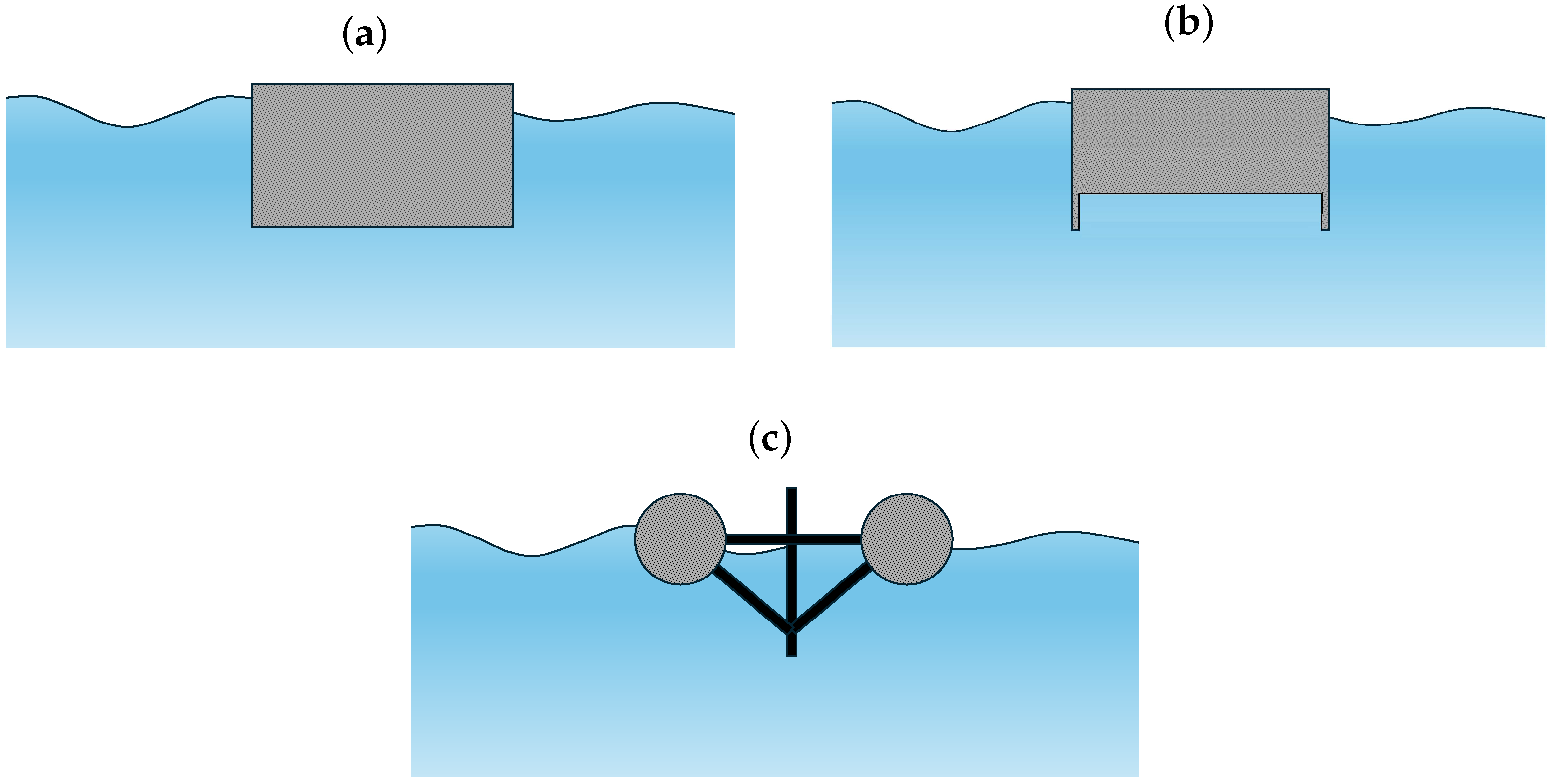
2. Cylindrical FBs
3. Physical Modeling
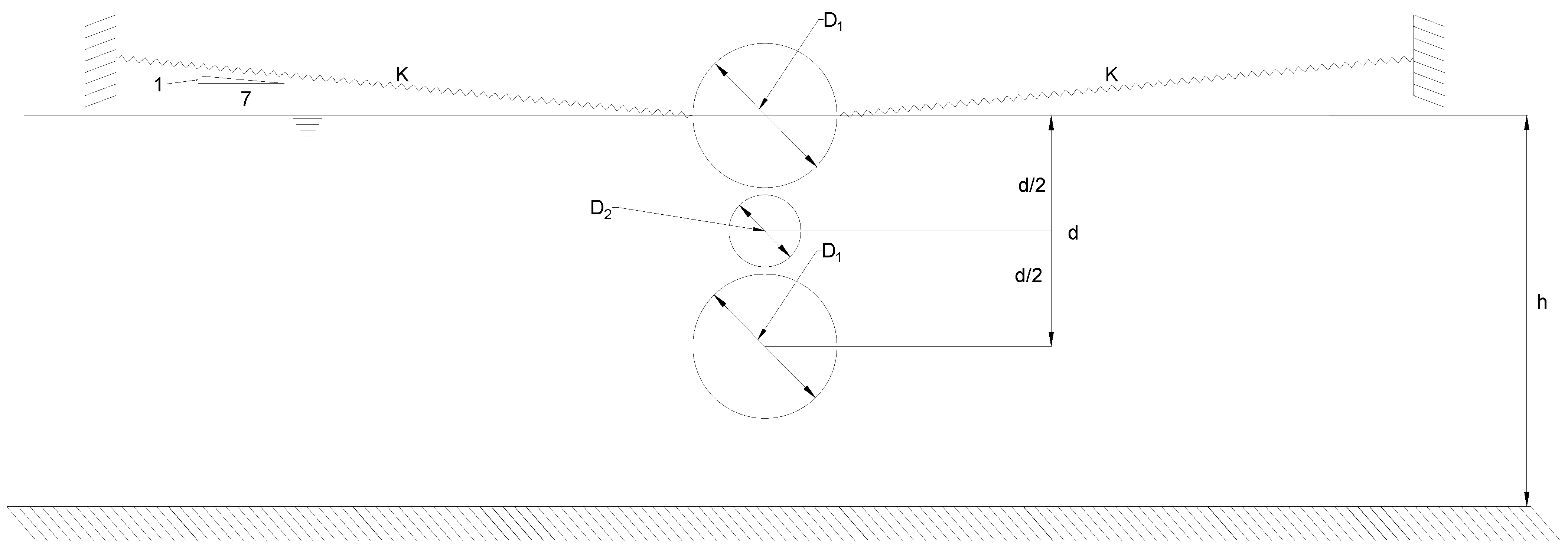
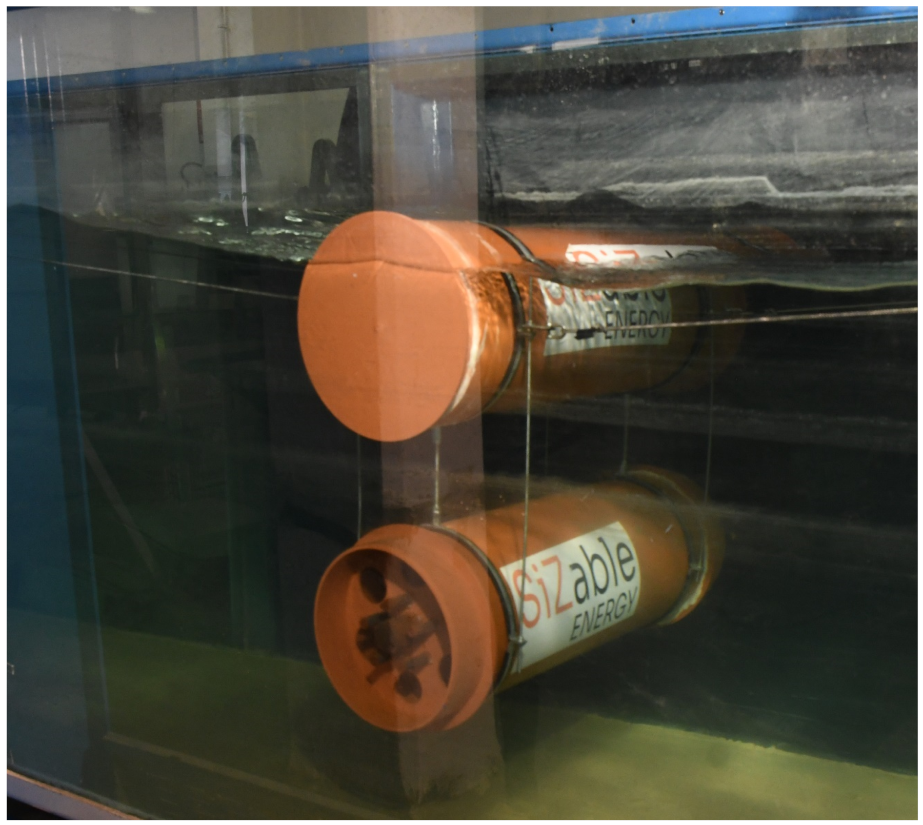
3.1. Test Description
- The incident, reflected, and transmitted waves through two arrays of four resistive wave gauges (WGs) placed in front of (offshore) and behind (shoreward) the FB, logged at 100 Hz;
- The load along the four mooring lines, through four full bridge load cells with maximum load 250 N, analog lowpass-filtered at 500 Hz and subsequently logged at 1200 Hz;
- The movements in sway, heave, and roll, captured by a two-megapixel webcam placed in front of the glass, recorded at 60 fps.
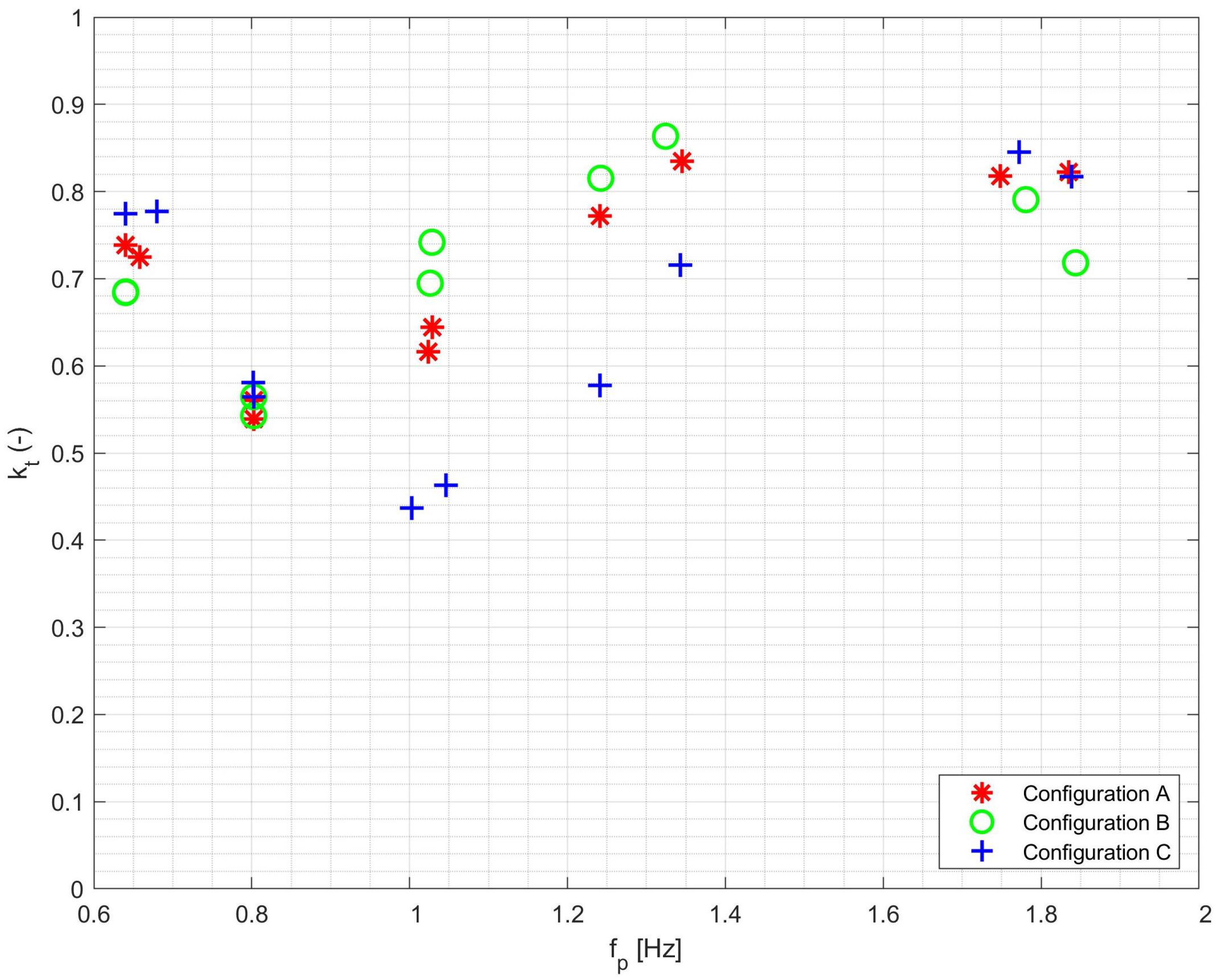
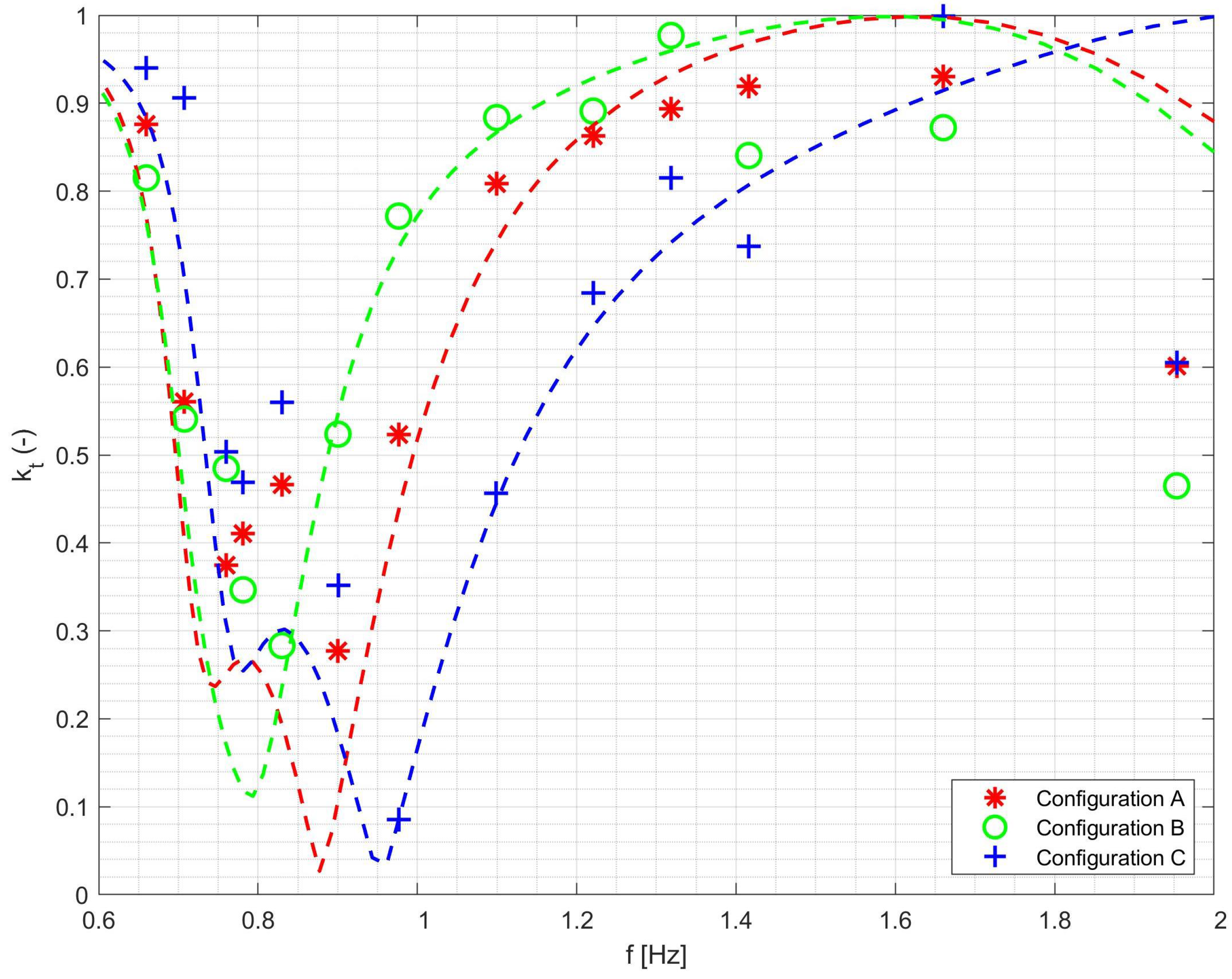
3.2. Results in Terms of Wave Transmission
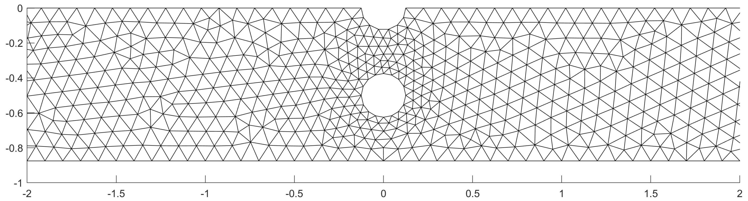
4. Numerical Model
Data Used in the Numerical Model
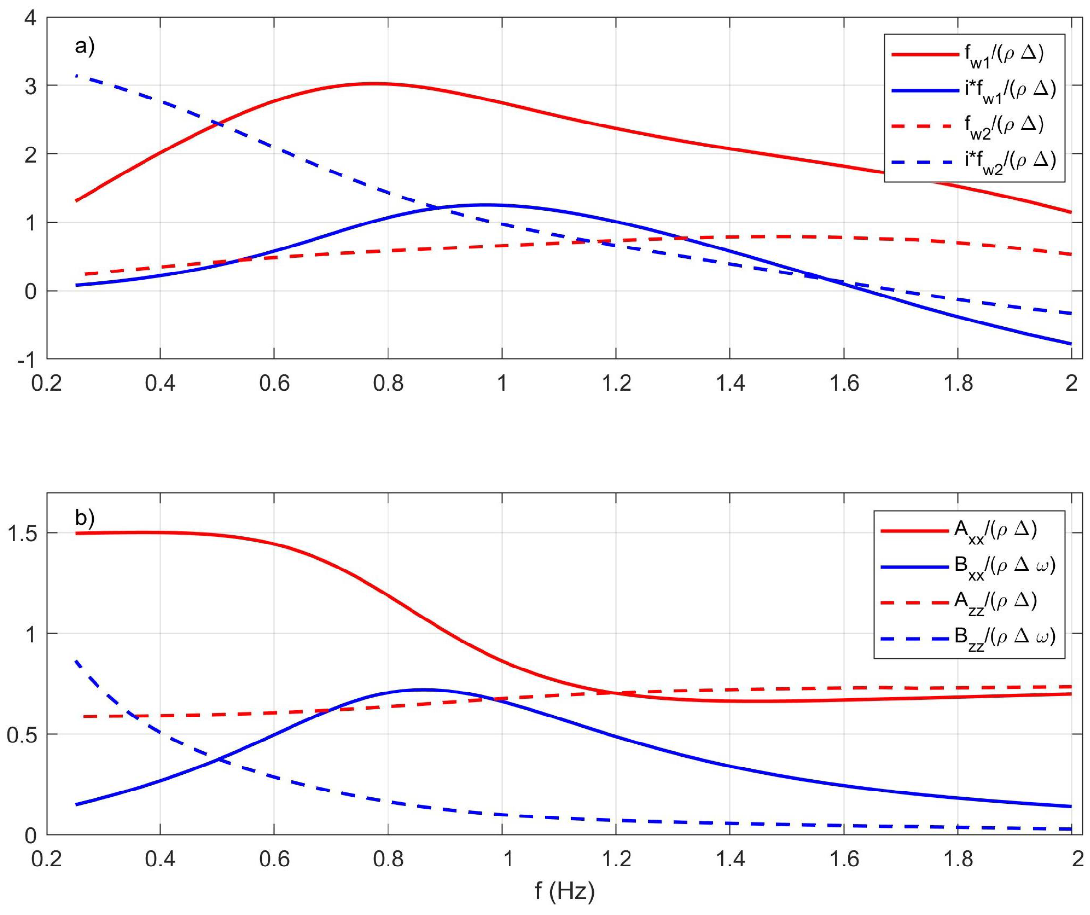
5. Numerical Interpretation
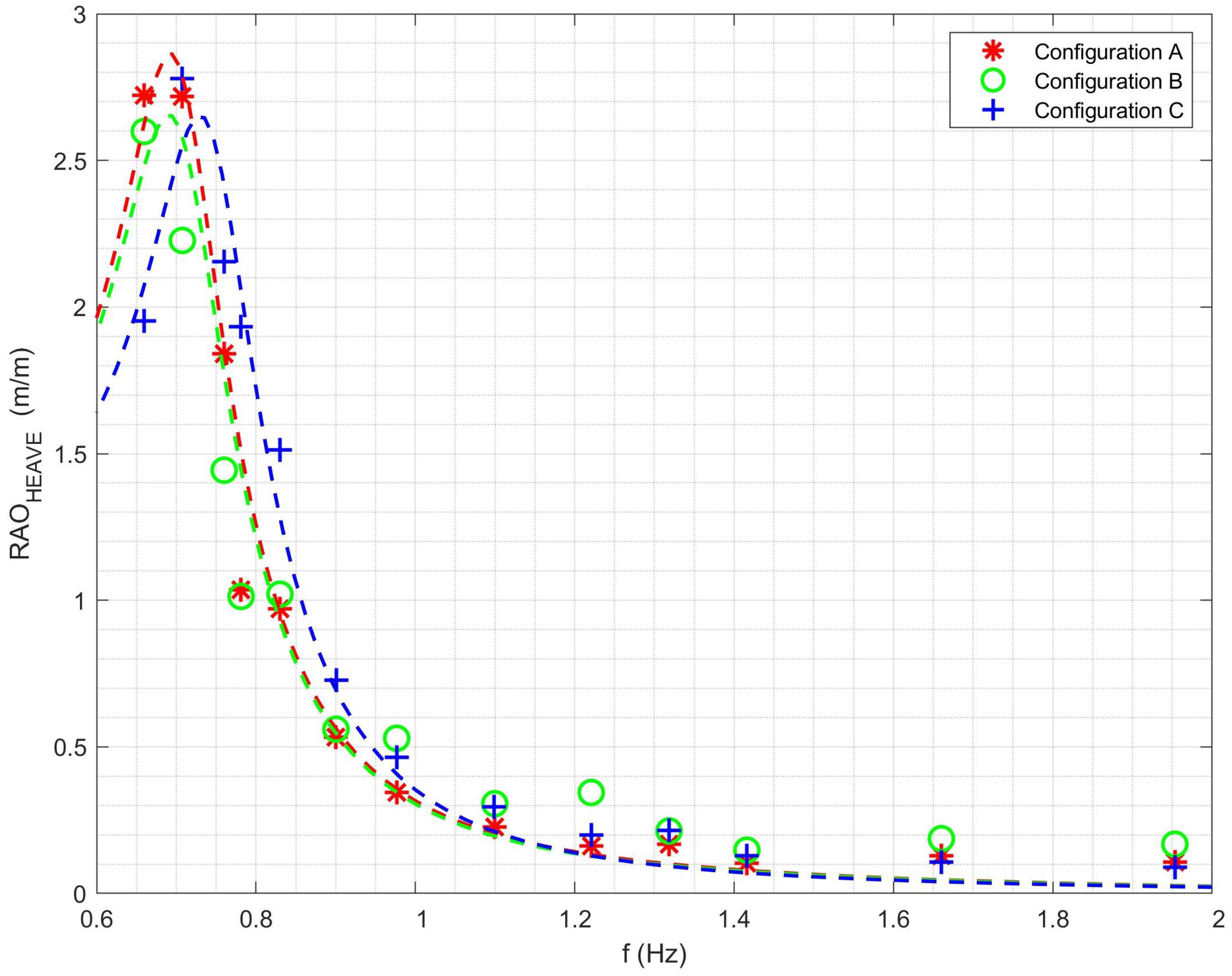
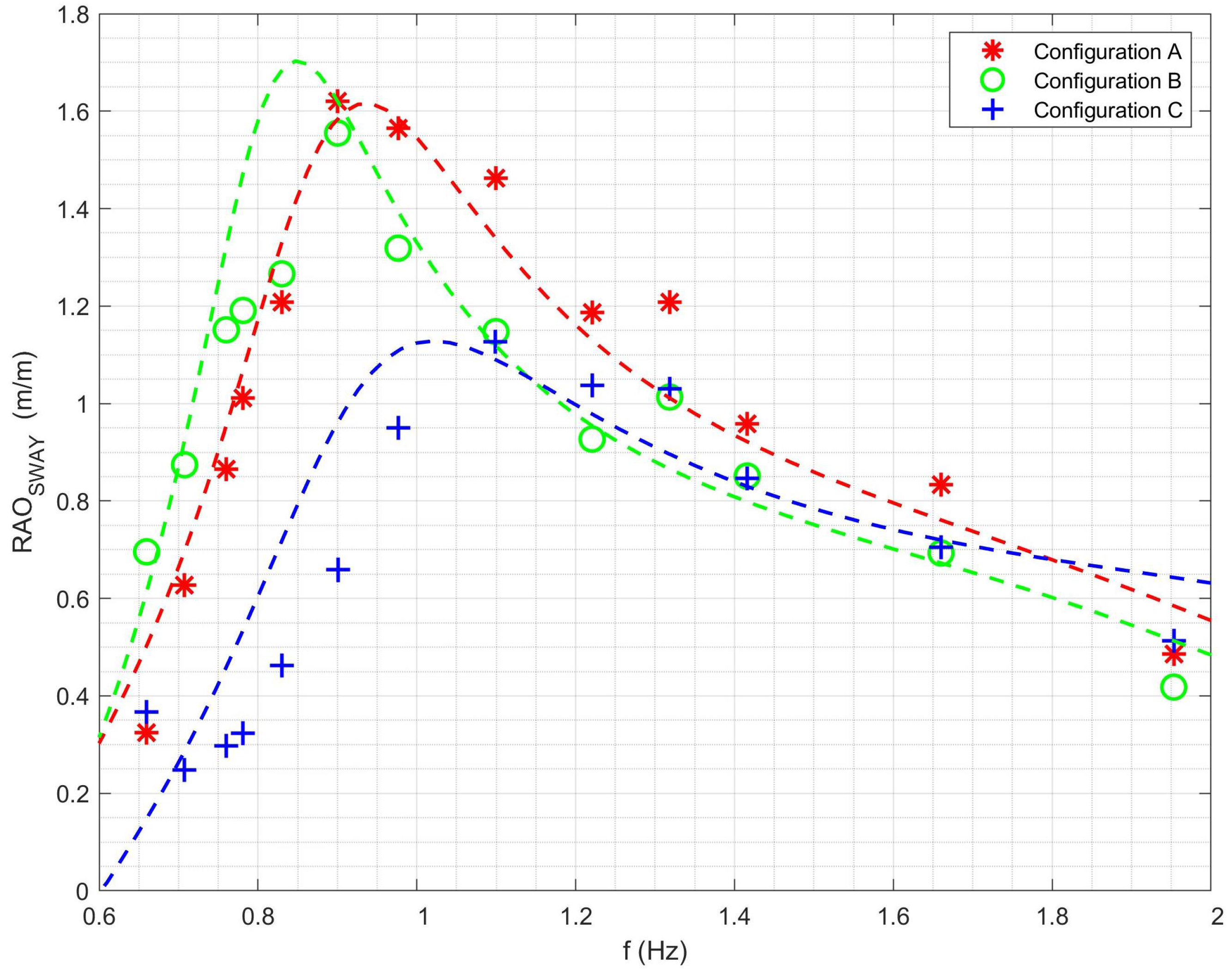
5.1. Measured Oscillations
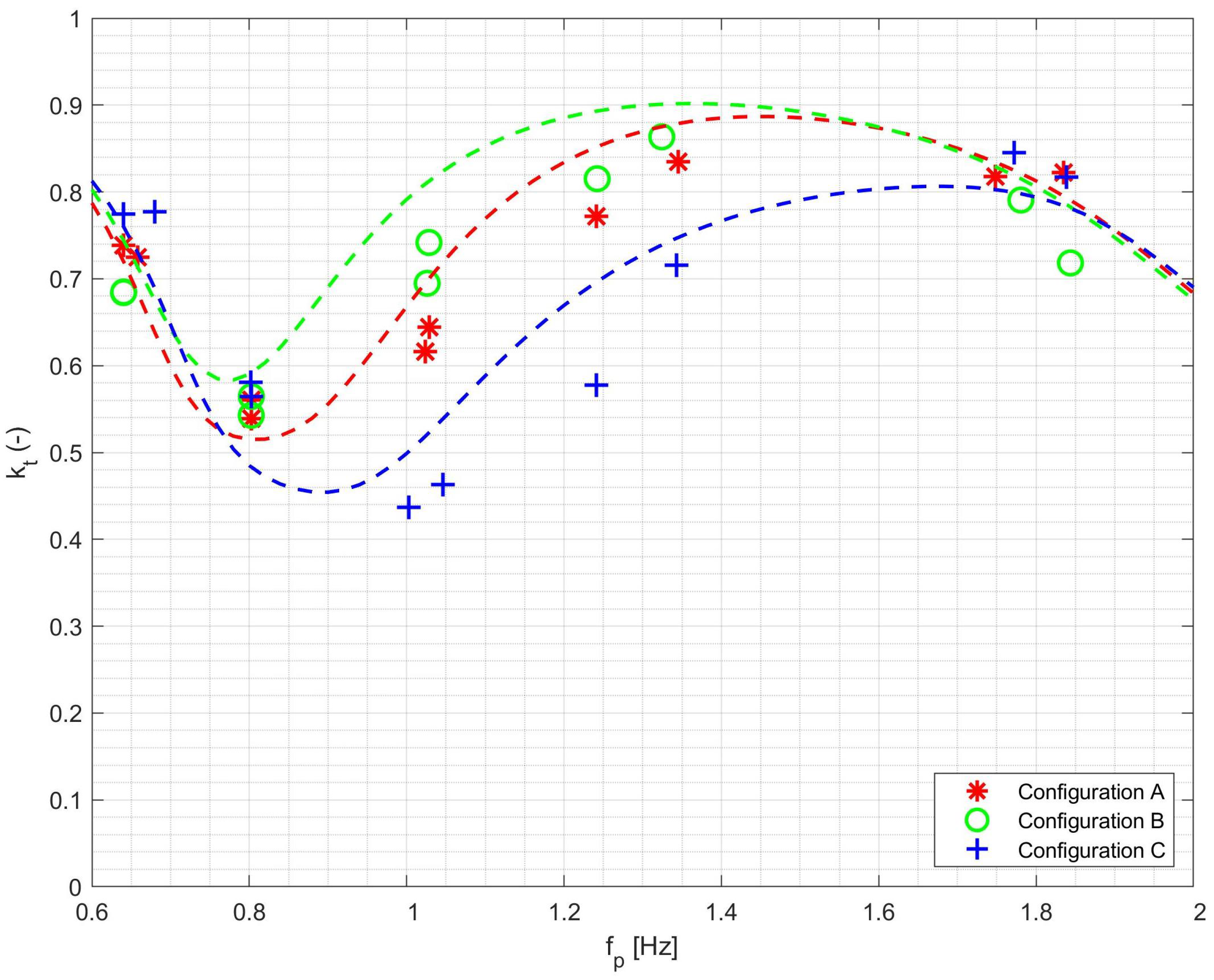
5.2. Measured Wave Transmission
5.3. Sensitivity Analyses
6. Conclusions
Author Contributions
Funding
Data Availability Statement
Conflicts of Interest
Abbreviations
| CG | Center of Gravity |
| DoF | Degree of Freedom |
| FB | Floating Breakwater |
| HDPE | Extruded High-Density Polyethylene |
| RAO | Response Amplitude Operator |
Appendix A. Numerical Model

- (i)
- (ii)
- (iii)
- Find the frequency domain responses using Equation (A9) and hence the RAOs.
- (iv)
- Compute the body velocity by Equation (A10).
- (v)
- Build the actual velocity potential as the sum of the incident, diffracted, and radiated potentials (the unit radiation multiplied by the computed body velocity) as shown in Equation (Figure 3).
- (vi)
- Extract from the actual velocity potential the transmitted and incident wave height, and hence .
References
- Smith, K.N. After D-Day, These Floating Harbors Helped Win WWII. Forbes, 6 June 2021. Available online: https://www.forbes.com/sites/kionasmith/2021/06/06/after-d-day-these-floating-harbors-helped-win-wwii (accessed on 20 June 2023).
- Katoh, J. Assessment of floating breakwaters. In Marine Behaviour and Physiology; Taylor & Francis _Eprint: Abingdon, UK, 1992; Volume 20, pp. 1–212. [Google Scholar] [CrossRef]
- Dai, J.; Wang, C.M.; Utsunomiya, T.; Duan, W. Review of recent research and developments on floating breakwaters. Ocean Eng. 2018, 158, 132–151. [Google Scholar] [CrossRef]
- McCartney, B.L. Floating breakwater design. J. Waterw. Port Coast. Ocean Eng. 1985, 111, 304–318. [Google Scholar] [CrossRef]
- Oliver, J.; Aristaghes, P.; Cederwall, K.; Davidson, D.; De Graaf, F.; Thackery, M.; Torum, A. Floating Breakwaters: A Practical Guide for Design and Construction. Available online: https://www.pianc.org/publication/floating-breakwaters-a-practical-guide-for-design-and-construction/ (accessed on 31 August 2024).
- Macagno, E. Fluid mechanics—Experimental study of the effects of the passage of a wave beneath an obstacle. In Proceedings of the Academic des Sciences, Paris, France, 19–24 June 1953. [Google Scholar]
- Brebner, A.; Ofuya, A.O. Floating Breakwaters. Coast. Eng. Proc. 1968, 1, 68. [Google Scholar] [CrossRef]
- Hom-ma, M.; Horikawa, K.; Mochizuki, H. An experimental study on floating breakwaters. Coast. Eng. Jpn. 1964, 7, 85–94. [Google Scholar] [CrossRef]
- Katō, J.; Hagino, S.; Uekita, Y. Damping effect of floating breakwater to which anti-rolling system is applied. In Coastal Engineering 1966; ASCE: Reston, VA, USA, 1967; pp. 1068–1078. [Google Scholar]
- Ruol, P.; Martinelli, L.; Pezzutto, P. Formula to predict transmission for π-type floating breakwaters. J. Waterw. Port Coast. Ocean Eng. 2013, 139, 1–8. [Google Scholar] [CrossRef]
- Ji, C.Y.; Chen, X.; Cui, J.; Gaidai, O.; Incecik, A. Experimental study on configuration optimization of floating breakwaters. Ocean Eng. 2016, 117, 302–310. [Google Scholar] [CrossRef]
- Dobnigg, A. Three 350-m-Long, Large Diameter HDPE Pipes Travel the Atlantic to be Sunk in the Caribbean. Available online: https://www.pipelife.com/content/wps/wpsint/main-website/en/service/news-and-projects/large-diameter-hdpe-pipes-travel-the-atlantic-to-be-sunk-in-the-caribbean.html/ (accessed on 31 August 2024).
- Ursell, F. On the heaving motion of a circular cylinder on the surface of a fluid. Q. J. Mech. Appl. Math. 1949, 2, 218–231. [Google Scholar] [CrossRef]
- Dean, R.G.; Ursell, F. Interaction of a Fixed, Semi-Immersed Circular Cylinder with a Train of Surface Waves; Massachusetts Institute of Technology, Hydrodynamics Laboratory: Cambridge, MA, USA, 1959. [Google Scholar]
- Yu, Y.; Ursell, F. Surface waves generated by an oscillating circular cylinder on water of finite depth: Theory and experiment. J. Fluid Mech. 1961, 11, 529–551. [Google Scholar] [CrossRef]
- Borgman, L. Computation of the Ocean Forces on an Infinitely Long Circular Cylinder in an Oblique Sea. Trans. Am. Geophys. Union 1958, 39, 885–888. [Google Scholar]
- Frank, W. Oscillation of Cylinders in or below the Free Surface of Deep Fluids; Naval Ship Research and Development Center: Washington, DC, USA, 1967; Volume 2375. [Google Scholar]
- Yeung, R.W. Added mass and damping of a vertical cylinder in finite-depth waters. Appl. Ocean Res. 1981, 3, 119–133. [Google Scholar] [CrossRef]
- Martin, P.A.; Dixon, A.G. The scattering of regular surface waves by a fixed, half-immersed, circular cylinder. Appl. Ocean Res. 1983, 5, 13–23. [Google Scholar] [CrossRef]
- Wang, S.; Wahab, R. Heaving oscillations of twin cylinders in a free surface. J. Ship Res. 1971, 1, 33–48. [Google Scholar]
- Bihs, H.; Ong, M.C. Numerical simulation of flows past partially-submerged horizontal circular cylinders in free surface waves. In Proceedings of the International Conference on Offshore Mechanics and Arctic Engineering, Nantes, France, 9–14 June 2013; American Society of Mechanical Engineers: New York, NY, USA, 2013; Volume 55416, p. V007T08A036. [Google Scholar]
- Ong, M.C.; Kamath, A.; Bihs, H.; Afzal, M.S. Numerical simulation of free-surface waves past two semi-submerged horizontal circular cylinders in tandem. Mar. Struct. 2017, 52, 1–14. [Google Scholar] [CrossRef]
- Cheng, X.; Liu, C.; Zhang, Q.; He, M.; Gao, X. Numerical Study on the Hydrodynamic Characteristics of a Double-Row Floating Breakwater Composed of a Pontoon and an Airbag. J. Mar. Sci. Eng. 2021, 9, 983. [Google Scholar] [CrossRef]
- Deng, X.; Liu, S.; Ong, M.C.; Ji, C. Numerical simulations of free-surface waves past two vertically aligned horizontal circular cylinders. Ocean Eng. 2019, 172, 550–561. [Google Scholar] [CrossRef]
- Dixon, A.G.; Salter, S.H.; Greated, C.A. Wave Forces on Partially Submerged Cylinders. J. Waterw. Port Coast. Ocean Div. 1979, 105, 421–438. [Google Scholar] [CrossRef]
- Ozeren, Y.; Wren, D.G.; Altinakar, M.; Work, P.A. Experimental Investigation of Cylindrical Floating Breakwater Performance with Various Mooring Configurations. J. Waterw. Port Coast. Ocean Eng. 2011, 137, 300–309. [Google Scholar] [CrossRef]
- Akgul, M. Effect of Pipe Spacing on the Performance of a Trimaran Floating Pipe Breakwater. In Proceedings of the ISOPE 2016, Rhodes, Greece, 26 June–1 July 2016. [Google Scholar]
- Kagemoto, H.; Yue, D.K. Interactions among multiple three-dimensional bodies in water waves: An exact algebraic method. J. Fluid Mech. 1986, 166, 189–209. [Google Scholar] [CrossRef]
- Abul-Azm, A.G.; Gesraha, M.R. Approximation to the hydrodynamics of floating pontoons under oblique waves. Ocean Eng. 2000, 27, 365–384. [Google Scholar] [CrossRef]
- Gesraha, M.R. Analysis of Π shaped floating breakwater in oblique waves: I. Impervious rigid wave boards. Appl. Ocean Res. 2006, 28, 327–338. [Google Scholar] [CrossRef]
- Martinelli, L.; Ruol, P.; Zanuttigh, B. Wave basin experiments on floating breakwaters with different layouts. Appl. Ocean Res. 2008, 30, 199–207. [Google Scholar] [CrossRef]
- Zelt, J.; Skjelbreia, J.E.; Wave, T. Estimating incident and reflected wave fields using an arbitrary number of wave gages. In Proceedings of the International Conference on Computers in Education (ICCE), Singapore, 7–10 December 1992; World Scientific Pub Co Inc.: Singapore, 1993; Volume 1, pp. 777–788. [Google Scholar]
- Falnes, J. Ocean Waves and Oscillating Systems: Linear Interactions Including Wave-Energy Extraction; Cambridge University Press: Cambridge, UK, 2002. [Google Scholar] [CrossRef]
- Kramer, M.B.; Andersen, J.; Thomas, S.; Bendixen, F.B.; Bingham, H.; Read, R.; Holk, N.; Ransley, E.; Brown, S.; Yu, Y.H.; et al. Highly Accurate Experimental Heave Decay Tests with a Floating Sphere: A Public Benchmark Dataset for Model Validation of Fluid–Structure Interaction. Energies 2021, 14, 269. [Google Scholar] [CrossRef]
- MathWorks, Inc. Image Processing Toolbox Reference; MathWorks, Inc.: Natick, MA, USA, 2024; Available online: www.mathworks.com (accessed on 15 June 2024).
- Brebbia, C.A.; Walker, S. Boundary Element Techniques in Engineering; Elsevier: Amsterdam, The Netherlands, 2016. [Google Scholar]
- Sjökvist, L.; Göteman, M.; Rahm, M.; Waters, R.; Svensson, O.; Strömstedt, E.; Leijon, M. Calculating buoy response for a wave energy converter—A comparison of two computational methods and experimental results. Theor. Appl. Mech. Lett. 2017, 7, 164–168. [Google Scholar] [CrossRef]
- Visbech, J.; Engsig-Karup, A.P.; Bingham, H.B. Solving the complete pseudo-impulsive radiation and diffraction problem using a spectral element method. Comput. Methods Appl. Mech. Eng. 2024, 423, 116871. [Google Scholar] [CrossRef]


| Configurations | (mm) | (mm) | d (mm) | h (mm) | K (N/m) |
|---|---|---|---|---|---|
| Config. A | 250 | None | 400 | 875 | 1200 |
| Config. B | 250 | 125 | 400 | 875 | 1200 |
| Config. C | 250 | none | 300 | 875 | 1200 |
| Configurations | A | B | C |
|---|---|---|---|
| Mass (kg) | 77.7 | 87.2 | 77.7 |
| Inertia (kg·m2) | 13.15 | 13.44 | 6.95 |
| Volume (m3) | 0.0736 | 0.0831 | 0.0736 |
| (m) | 0.380 | 0.370 | 0.285 |
| (m) | 0.266 | 0.256 | 0.200 |
Disclaimer/Publisher’s Note: The statements, opinions and data contained in all publications are solely those of the individual author(s) and contributor(s) and not of MDPI and/or the editor(s). MDPI and/or the editor(s) disclaim responsibility for any injury to people or property resulting from any ideas, methods, instructions or products referred to in the content. |
© 2024 by the authors. Licensee MDPI, Basel, Switzerland. This article is an open access article distributed under the terms and conditions of the Creative Commons Attribution (CC BY) license (https://creativecommons.org/licenses/by/4.0/).
Share and Cite
Martinelli, L.; Mohamad, O.; Volpato, M.; Eskilsson, C.; Aufiero, M. Attenuation Capacity of a Multi-Cylindrical Floating Breakwater. J. Mar. Sci. Eng. 2024, 12, 1550. https://doi.org/10.3390/jmse12091550
Martinelli L, Mohamad O, Volpato M, Eskilsson C, Aufiero M. Attenuation Capacity of a Multi-Cylindrical Floating Breakwater. Journal of Marine Science and Engineering. 2024; 12(9):1550. https://doi.org/10.3390/jmse12091550
Chicago/Turabian StyleMartinelli, Luca, Omar Mohamad, Matteo Volpato, Claes Eskilsson, and Manuele Aufiero. 2024. "Attenuation Capacity of a Multi-Cylindrical Floating Breakwater" Journal of Marine Science and Engineering 12, no. 9: 1550. https://doi.org/10.3390/jmse12091550